UNIVERSITÉ
DU QUÉBEC À
MONTRÉAL
OPTIMISATIO DE L'APPROCHE DE LA RÉDUCTION D
'ÉCHELLE
MULTIPLE POUR RÉALISER UNE
PROJECTION
CLIMATIQUE
DE LA
PRÉCIPITATION
MIXTE
À HAUTE RÉSOLUTION
THÈSE
PRÉSENTÉE
COMME EXIGENCE
PARTIELLE
DU DOCTORAT El
SCIE CES
DE LA
TERRE ET
DE L'ATMOSPHÈRE
PAR
DOMINIC
MATTE
UNIVERSITÉ DU QUÉBEC À MONTRÉAL Service des bibliothèques
Avertissement
La diffusion de cette thèse se fait dans le respect des droits de son auteur, qui a signé le formulaire Autorisation de reproduire et de diffuser un travail de recherche de cycles supérieurs (SDU-522 - Rév.0?-2011 ). Cette autorisation stipule que «conformément
à
l'article 11 du Règlement no 8 des études de cycles supérieurs, [l'auteur] concèdeà
l'Université du Québecà
Montréal une licence non exclusive d'utilisation et de publication de la totalité ou d'une partie importante de [son] travail de recherche pour des fins pédagogiques et non commerciales. Plus précisément, [l'auteur] autorise l'Université du Québec à Montréalà
reproduire, diffuser, prêter, distribuer ou vendre des copies de [son] travail de rechercheà
des fins non commerciales sur quelque support que ce soit, y compris l'Internet. Cette licence et cette autorisation n'entraînent pas une renonciation de [la] part [de l'auteur] à [ses] droits moraux ni à [ses] droits de propriété intellectuelle. Sauf entente contraire, [l'auteur] conserve la liberté de diffuser et de commercialiser ou non ce travail dont [il] possède un exemplaire.»UNIVERSITY OF QUÉBEC AT MONTRÉAL
OPTIMIZATION OF THE MULTIPLE ESTING APPROACH TO REALIZE A CLIMATE PROJECTION OF MIXTE PRECIPITATION AT HIGH RESOLUTION
THESIS PRESENT
AS PARTIAL REQUIREMENT OF THE DOCTORATE IN EARTH AND ATMOSPHERIC SCIENCES
BY
DOMINIC MATTE
REMERCIEMENTS
De par les grandes difficultés techniques, professionnell s et r lationnelles qu'un parcours doctoral peut comporter, il est assez peu probable d'y arriver sans aide. Cette thèse n'en fait pas exception et doit son accomplissement grâce à l'aide de plusieurs peronne .
Mes premiers remerciements vont à mon directeur de thèse René Laprise qui a été pour moi non seulement une grande source d'information, mais aussi d'inspiration. Je le remercie pour ses muliples conseils (autant scientifique que personnels), sa très grande rigueur, son support et la grande liberté qu'il m'a lai sée. Bien que la fin d'un tel projet me procure une grande joie, elle m'attriste tout autant, car elle met fin à une relation directeur-étudiant que je chérissais.
Mes seconds remerciements vont à ma codirectrice de th' se, Julie M. Thériault. Je la remercie pour a grande rigueur, son enthousiasme, ses conseils et sa patience. Ses conseils scientifiques m'ont permis d'atteindre une qualité exceptionnelle dans les divers travaux que nous avons réalisés ensemble.
Un grand merci à Mélissa Cholette pour son support et ses conseils toujours d'une grande pertinence. Merci à Katja Winger pour ses conseils, sa patience sans limites et son enthousiasme; à Bernard Dugas pour ses précieux conseils sur le MRCC5; à Olek-sandr (Sasha) Huziy pour ses conseils techniques. Merci aussi à Guillaume Dueymes, Frédéric Chosson, Emmanuel Poan pour leur support, leurs conseils et leur amitié.
Je remercie également la faculté des sciences de l'UQA f pour m'avoir décerné le prix 2017 de la meilleure publication scientifique étudiante.
Je remercie aussi ma conjointe Luce; merci sans toi rien de ceci ne serait possible! Finalement, un dernier remerciement à ma défunte mère, mon p' re, mes frères et mes ami( e)s pour tout le plaisir que vous me procurez.
TABLE
DES MATIÈRES
REMERCIEMEI TS . . LISTE DES FIGURES RÉSUMÉ ..
ABSTRACT
CONTRIBUTIONS À LA SCIENCE .
co
TRIBUTIONS PERSO NELL ES INTRODUCTION . . .0.1 Objectifs et Approche CHAPITRE I
COMPARISON BETWEEN RICH-RESOLUTION CLIMATE SIMULATIONS USING SINGLE AND DOUBLE ESTII G APPROACHES WITHIN THE BI
G-Ill VIl xv XVII xix XXI 1 4
BROTHER EXPERIME TAL PROTOCOL 6
1.1 Introduction. . . . 8
1.2 Mode! description 10
1.3 Experimental design 10
1.3.1 Single nesting approach 1.3.2 Double nesting approach 1.4 Analysis tools .
1.5 Results . . . .
1.5.1 Stationary component 1.5.2 Transient-eddy component
1.5.3 Single nesting VS Double nesting .
12 12 12 14 14 15 16
1.6 Summary and Discussions 17
1.7 Appendix . . . . . . . . . 20
1.8 Appendix [Step A]: The optimum domain for the intermediate-resolution simulation . . . . . . . . . . . . . . . . . . . . . . . . . . . . . . . . . 21
vi
1.9 Appendix [Step B]: The optimum large-scale spectral nudging . . . . . . . . 23 1.10 Appendix [Step
C]:
Optimal fil ter to reproduce the variance spectrum of a0.45°-mesh simulation . . . . . . . . . . . . . . . . . . . . . . . . 24 CHAPITRE II
SPATIAL SPIN-UP OF FINE SCALES IN A REGIONAL CLIMATE MODEL SIMULATION DRIVEN BY LOW-RESOLUTION BOUNDARY CONDITIONS 37 2.1 Introduction . . .
2.2 Experimental design 2.3 Results . .
2.4 Conclusion
2.5 Appendix: Spatial spin-up and ne ting interval CHAPITRE III
CLIMATE CHA GE STUDY OF J\!IIXED PRECIPITATION OVER SOUTH-39 40 42 46 48
ERN QUÉBEC USL GA REGIONAL CLIMATE MODEL 59
3.1 Introduction . . . 3.2 Exp rimental design
3.2.1 CRCM5 configuration 3.2.2 Hindcast simulation setup
3.2.3 Historical and projected climatc simulations setup 3.2.4 Diagnostic of precipitation types
3.2.5 Available Observations . 3.2.6 Methodology . . . .
3.3 Pa t climatology of mixed precipitation 3.3.1 Occurrence of mixed pr cipitation
61 63 63 64 64 65 66 66 67 67 3.3.2 Atmospheric conditions a ·sociated with long-and hort-cluration events 68 3.3.3 Seasonal variation . . .
3.4 Projected climate change of mixecl precipitation . 3.5 Conclusions . . .
3.5.1 The hindcast simulation
3.5.2 The historical and projectecl future climate.
69 70 71 71 72
VIl
3.6 Appendix: Vertical profiles 74
3.7 Appendix: Historical Simulation 75
3.8 Appendix: Spatial variability 75
LISTE DES F
IGURES
1.1 The experimental fiowchart. Era-interim (ERAI) is usecl to drive the CRCM5 on a 0.15° mesh (RCM.15), the result is the Big-Brother simula-tion (BB.15). This simulation is usecl as reference to valiclate the Littl e-Brother (LB) simulation and also processecl by a low-pass filter creating BB.15_Fl.8, which is u ·ecl as clriving data for the two approaches. For the single nesting, the BB.15_Fl.8 clataset is usecl to drive the CRCM5 on a 0.15° mesh (CRCM5.15) on multiple domain size (Di) with the same con-figuration usecl to simulate BB.15. The resulting clatasets (LB.15_LDi: Little-Brothcr simulations for the i domain sizes of the single n sting ( Fig.1.2)) are comparecl to BB.15. For the double nesting, the BB.15_Fl.8 clataset i usecl to creatc the surr·ogate intermecliate simulation (Surro-gate.45: see Appenclix) that provicles the SB.45 clataset usecl to drive the CRCM5 on a 0.15° mesh (CRCM5.15) on multiple domain ize (Dj) with the same configuration u ecl to simulate BB.15 (LB.15_2_Dj: Little-Brother simulations for the j domain sizes of the double nesting (sec Fig.1.2)) are comparecl to BB.15 and LB.15_LDi. . . . . . . . . . . . 25 1.2 The simulation clomains for the BB.15 (760 x 760 gricl points), the LBs
with domain size of 460 x 460, 260 x 260, 160 x 160, 110 x 110 and 60 x 60 gricl points for the single nesting (Fig.l.l: LB.15_LDi) and 260 x 260, 160 x 160, 110 x 110 and 60 x 60 gricl points for the double n sting (Fig.l.l: LB.15_2...Dj). Climate statistics were computecl in the black clashecl square area of 44 x 44 gricl points. . . . . . . . . . . 26 1.3 Filtcr rcspon c for the BB filtcr (red line) and the analysis filter (black
line). . . . . . . . . . . . . . . . . . . . . . . . . . 27 1.4 Large-scale stationary component of the mean sea leve! pressure (a) and
850-hPa relative humiclity (b) fields. The clots correspond to the single-nesting results and the crosses to the clouble-nesting results. The colour correspond to the varions domain sizes of the LB. The blue clot co rre-sponds to the reference BB.15 simulation. . . . . . . . . . . 28 1.5 Spatial mean of the largc-scale transient-eclcly component of 300-hPa
meridional wincl (a) and 50-hPa relative humiclity (b). . . . . . 29 1.6 Small-. cale transient-eclcly component of 700-hPa relative vorticity (a)
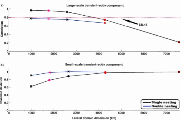
1.7 Transient-eddy statistics for the single nesting (solid black line) and the double nesting (solid blue line). The first figure (a) repre ent the large-scale transient-eddy correlation and the second figure (b) the small- cale transient-eddy standard deviation for the relative humidity at 700 hPa by the lateral domain dimension (km). The magenta dashed line represents
IX
the large-scale transient-eddy correlation of the SB.45 simulation. . . . . 31 1.8 Same as Fig.l.7 but with large-scale spectral nudging activated in
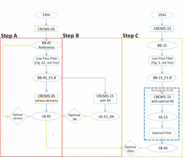
gener-ating the LBs. The SN was applied to horizontal wind components with horizontal length scales larger than 1000 km, with a recall strength set to zero below the 850-hPa leve!, then increasing linearly toits maximum value at 500 hPa, and remaining constant to the mode! top leve!. The spectral nudging maximum strength is 1.3o/c applied at each time step. . 32 1.9 Flowchart of the protocol for the surrogate simulation. For the step A,
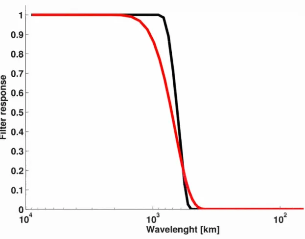
Era-Interim (ERAI) i used to drive the CRCM5 at 0.45° mesh (CRCM5. -45), the result is the Big-Brother simulation (BB.45). This simulation is used as reference to validate the Little-Brother (LB.45) simulation and also processed by a low-pass filter creating BB.45_Fl.8 that is used as driving data for the CRCM5 (CRCM5.45; varions domain ) on var-ions domain sizes with the same configuration used to imulate BB.45. The resulting datasets (LB.45) are compared to BB.45 to highlight the optimal domain size. For the step B, BB.45_Fl.8 is used to drive the CRCM5 (CRC /[5.45; with SN) on a unique domain size with different spectral nudging configurations. The large scales of the resulting datasets (LB.15_S ) are compared with optimal domain size simulation from the previous step. For the tep C, Era-Interim (ERAI) is used to drive the CRCM5 at 0.15°-mesh (CRCM5.15), the result is the Big-Brother simu-lation (BB.15: same as in section 3). This simulation is processed by a low-pass filter creating BB.15_Fl.8 (same as in section 3) which is used as driving data for the CRCM5 at 0.15°-mesh with the optimal spectral nudging configuration highlights in step B (CRCM5.15; with optimal SN). The resulting dataset (SB.15) has been processed by severa! spectral fil-ters and results compared to the variance spectrum of LB.45 in order to find the optimal spectral filter. The results dataset is the surrogate simulation (SB.45) as presented in Fig.l.l. . . . . . . . . . . . . . 33 1.10 Filter response for the BB filter (red line) and the analysi filter (black
line). . . . . . . . . . . . . . . . . . . . . . . . . . . . . . . . . 34 1.11 Relative humidity statistics from the Big-Brother experiment realized at
0.45° mesh for the stationary component of the original fields at 850 hPa (a) and the tran ient-eddy component of the small-scale field at 700 hP a (b ). . . . . . . . . . . . . . . . . . . . . . . . . . . . . . . . . 35
1.12 Kinetic energy spectrum for the 700-200 hPa atmospheric layer, averaged for 1997, 1998, 1999 and 2000, for the various simulations. The red line corresponds to 0.45°-mesh simulation driven by BB.45_Fl.8 (notee! LB.45 in Fig.l.9), the black line to the 0.15°-mesh simulation with optimal SN parameters driven by BB.15_Fl.8 (notee! SB.l5 in the Fig.l.9), and the blue li ne the optimally filtered version of the latter (notee! SB.45 in the
x
Fig.l.9). . . . . . . . . . . . . . . . . . . . 36 2.1 The domain of the Big-Brother simulation (BB)(free domain of 760 x 760
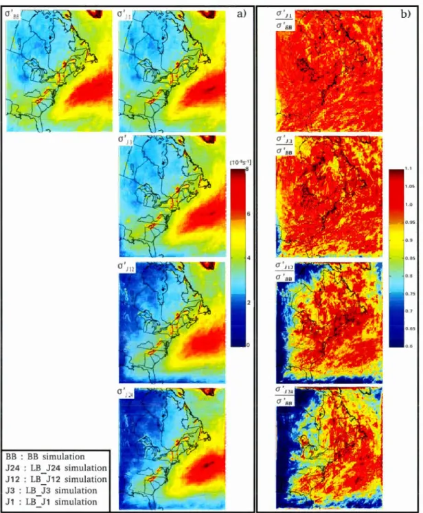
grid points). All the Little-Brother simulations have a free domain of 260 x 260 gr id points cent red on Montréal (D 1) . . . . . . . . . 51 2.2 Small-scale transient-eddy standard deviation of the 700-hPa relative vo
r-ticity for the four December simulation . b) Ratio of the LB simulations standard deviation with that of the reference BB simulation (
~',,.
) 52aaa 2.3 Same as Fig.2.2, but for the four July months.
2.4 a): ·west to East eut, across the domain, (a shawn at the bot tom right of panel a) of the small-scale transient-eddy standard deviation for the rela-tive vorticity at 700 hPa of LB_Ji normalized by the ref renee simulation BB, as a function of the distance from the western boundary (in km and number of grid points (n) in the upper and lovver ab ci a respectively in both panel), for the four months of December. The different jumps of resolution J24, J12, J3 and J1 are hown by the blue, red, green and black !ines, respectively. b) Same as a) but only for J12 at three different levels: 850 hPa (green), 700 hPa (red) and 500 hPa (blue).The empirical
53
equations (2.6) and (2.7) are indicated by the dash-d !ines . 54
2.5 Same as Fig.2.4 but the four July rnonths. . . . . 55 2.6 Equivalent to Fig. 4a, but for similar experiment realized with an RCl\I
on a 0.45° mesh rather than 0.15° mesh. . . . . . . . . . . 56 2.7 An abacus developcd from Eq.(2.6) and Eq.(2.7) showing the distance
3 L (right hanc! y-axis) and 3 N (solid black !ines) required to attain 95% of the asymptotic amplitude of the small-scale transient cddies, as a function of the grid mesh of the LBC (ordinate) and RCM (abscissa), respectively, for an average wind speed V equal to the typical speed of synoptic-scale weather systems C (V~C). . . . . . . . . 57 2.8 Same as Fig.2.4a but with a nesting time interval of 6 h. 58
3.1 The domain location for the different experimental setups. Panel (a) shows the domain location of the intermediate-resolution simulation (in blue) and the high-resolution simulation (in black) used for the two-step dynamical downscaling of the historical and climate-change simulations. The green square is the domain location used for the hindcast simula-tion. The color shadings represent the spatial spin-up region for each case. The red square represents the "trustworthy" region of a size of 80 x 90 gr id points. Panel (b) is the topography (grey shading) and the lo-cation of the MANOBS stations (red stars). The labeled ones are Pierre-Elliot Trudeau airport (YUL), Mirabel (YMX), Québec City (YQB) and
Xl
Bagotville (QBG) . . . . . . . . . . . . . . . . . . . . . . . . 77 3.2 Mean annual hourly occurrence of mixed precipitation diagnosed by a)
Bourgouin, b) Czys, c) Cantin and Bachand, d) Ramer, e) Baldwin, f) the average among the 5 algorithms and g) the standard deviation around their average. The stations are indicated by the white disks and the values are the same as the color bar. . . . . . . . . . . . . . . . . 78 3.3 Mean annual hourly occurrence of mixed precipitation of the observation
(black), and diagnosed by Bourgouin (red), Czys (green), Ramer (purple), CB (blue), and Baldwin (dark green), for the locations of Y fX, YUL, YQB and YBG, respectively. The black lines represent the standard deviation of the nine grid points nearest to the corresponding MAI OBS stations. . . . . . . . . . . . . . . . . . . . . . . . . . . . . . . . . . . . . 79 3.4 Histograms of the number of hours per mixed precipitation event in
dif-ferent time ranges; (a) from 1 to 10 hours; b) 11 to 30 hours and c) 31 to 60 hours, for Dorval (YUL, Figure 1) for the 5 algorithms: Bourgouin (red), Czys (lime green), Ramer (purple), CB (blue), and Baldwin (dark green). The black lin es re present the standard deviation of the ni ne gr id points nearest to the MANOBS station. . . . . . . . . . . . . . . . . 80
3.5 Composite analysis at the beginning of all short-duration (left column) and long-duration (right column) mixed precipitation events. Panels (a,b) show the mean sea leve! pressure (MSLP) in ERA-Interim, pa n-els ( c,d) show the simulated monthly 2-m temperature anomalies (co lor shading), the MSLP (black lines) and the 10-m wind speed and direction (barbs). The blue line is the 2-m 0°C isotherm. Panels (e,f) show the frequencies (%) of mixed precipitation when occurring at YUL, panels (g,h) show the vertical profile of horizontal wind speed and direction at YUL, and panels (i,j) show the 10-m wind roses, with the colors indicat -ing wind speed. The black star indicates the location of Dorval, Québec (YUL). . . . . . . . . . . . . . . . . . . . . . . . . . . . . 81
- - - --
-3.6 Monthly number of hours (!eft column) and the number of events (right column) for (a,b) YUL, (c,d) YMX, (e,f) YQB and (g,h) YBG. The black !ines correspond to the observed values while the colored !ines correspond to the mix d precipitation diagnos d by th various algorithms, Baur-gouin (red), Czys (lim gr en), Ram r (purple), CB (blue) and Baldwin (clark green). The dashed !ines and the plain !ines are the short- and long-duration events, re pectively . . . .
3.7 Annual number of hours (left column) and the number of events (right column) for the period of (a,b) 1980-2009, (c,d) the period of 2070-2099, and (e,f) the corre. ponding changes for short-duration events the average
xii
82
of the 5 algorithm . . . . . . . . . . . . . 83
3.8 Same as Fig.3.7, but for long-duration events 84
3.9 Climate change of monthly hours (left column) and number of events (right column) of mixed precipitation at (a,b) YUL, (c,d) YMX, (e,f) YQB and (g,h) YBG as diagno ·ed by Bourgouin (red), Czys (green), Ramer (purpl ), CB (blue), and the av rage of the 5 algorithms (black). 85 3.10 The vertical temperature profiles at t=Oh for short and long event of MP
when diagnosed by Bourgouin (a & b), Czys (c & d), Ramer (e & f), by Cantin & Bachand (g & h) and Baldwin (i & j). The blue and red !ines represent the cold and warm profiles respectively. The upper-right number is the
%
of cold profiles. . . . . . . . . . . . . 86 3.11 Number of hours per year for short-duration events (left column) andlong-duration events (right column) the average of the 5 algorithms in the reanalysi -driven hindcast simulation (a,b) CRCM5/ERA, CGCM-driven historical simulation ( c,cl) CRCM5/MPI, and ( e,f) their difference. 87 3.12 Number of events per year for short-duration events (!eft column) and
long-duration events (right column) the average of the 5 algorithms. in the reanalysi -driven bindcast simulation (a,b) CRCM5/ERA, CGCNI-driven historical simulation (c,cl) CRC:~vi5/MPI, and ( ,f) their difference. 88 3.13 Monthly number of hour (left column) and the number of events (right
column) for YUL as diagnosed by Bourgouin (a,b), Czys (c,d), Ramer (e,f), CB (g,h) and Baldwin (i,j) from the hindcast CRCi\I5/ERA sol u-tion. Th plum indicate th lowe t an l the highe t values at the nine grid points nearest to the YUL station. The black !ines and the clark colors correspond to the observed value and the simulated results, re-spectively, for th long-duration event . The da hec! !ines and the pale colors are the observed value and the imulated results, respectively, for the short-duration vents. . . . . . . . . . . . . . . . . . . . . . 89
LISTE DES ABRÉVIATIONS, SIGLES ET ACRONYMES AR5 BB BBE CF CGCM CLASS C IC CM
cc
Clv!RC CO RD EX CRCM5 DCT ERA-I GCM GE f GF IC IPCC J LB LBC LE MCG MetUM MP MRC MRCC5the Fifth Assessment Report
Big-Brother simulation
Big-Brother Experiment
Conditions aux frontières
Coupled Global Climate Madel
Canadian Land S Ltrface Scheme
Canadian Meteorological C ntre
Coût de calcul d'un MCG
Coût de calcul d'un MRC
COordinated R gional climate Downscaling Experiment Fifth-generation Canadian Regional Climate Mode!
Discrete Cosine Transform
Era-Interim reanalysis
Coupled Global Climate Mode!
Global Environnement Multiscale mode!
Simulation du grand frère
Initial Condition
Intergovernmental Panel on Climate Change
Jump of resolution between the driving data and the nested madel
Little-Brother simulation
Lateral Boundary Condition
Long-duration event
Modèle de circulation générale
Met Office United Mode!
Mixed precipitation
Modèle régional du climat
Cinquième génération du Modèle Régional Canadien du Climat Xlii
PF RCM RCP SB SE SLRV SN
ss
WRFSimulations du petit frère Regional Climate Mode!
Representative Concentration Pathway Step Brother simulation
Short-duration event St. Lawrence River Valley Spectral Nudging
Small Scales
Weather Research and Forecasting Mode!
RÉS
UMÉ
La précipitation verglaçante peut avoir des impacts néfastes sur la société, tels que
causer des pannes de courant majeures, ainsi que produire de sérieux problèmes dans les réseaux de transport. Malgré les conséquences catastrophiques associées à ce type de
précipitation, elle est encore peu étudiée dan un contexte de changement climatique.
Pour représenter ce type de précipitation dans les modèles du climat, il est important de
correctement simuler les écoulements atmosphériques près de la surface. Les simulations
climatiques à haute ré olution sont, donc, nécessaires pour représenter adéquatement
la topographie, mais ces dernières exigent des ressources informatiques considérables,
surtout lorsqu'on utili ·e des modèles de circulation générale. Or, les modèles régionaux du climat (MRC) ont des modèles à aire limitée qui permettent la simulation du climat
à fine échelle à un moindre coùt de calcul. Ces derniers utilisent les solutions des
modèles de circulation générale à leur frontières pour développer leurs propres solutions.
Cependant, lorsqu'ils sont utilisés à très haute résolution, le nombre de calculs requis
peut être hors de la portée de re om·ces informatiques disponibles. L'utilisation en
cascade d'un modèle régional du limat pourrait être une alternative pratique pour garder le coùt de calcul raisonnable. L'objectif principal de cette thèse est d'étudier et
optimiser l'utilisation de la réduction d'échelle dynamique multiple comme une approche
appropriée pour réali er une étude du climat de la précipitation verglaçante à faible coùt de calcul. Cette thèse est divisée en trois sections.
La première partie étudie l'approche de la cascade pour réaliser des simulations climatiques à haute résolution. Dans cette étude, des résultats de simulations obtenues avec une approche de réduction d'échelle simple et double sont comparés selon le pro-tocole expérimental "idéalisé" elu grand frère. Une première simulation, nommée la simulation elu grand frère, est réalisée sur un grand domaine à la résolution désirée. Cette simulation sert de référence. La solution du grand frère est ensuite traitée par un filtre passe-bas permettant de garder seulement les grandes échelles qui serviront de con-ditions aux frontières (CF) à des simulations tests appelées les simulations elu petit frère. Pour la réduction d'échelle simple, les imulations tests sont directement pilotées par la solution de la simulation de référence filtrée, alors que pour la réduction d'échelle double
un substitut d'une simulation de résolution intermédiaire est utilisé. L'étude de la
com-posante stationnaire montre très peu de différences entre les deux approches, alors que la composante de la variabilité transitoire montre de grandes différences. L'approche de la réduction d'échelle double dégrade légèrement les grandes échelles, mais permet une
importante réduction de la grandeur cl domaine requise pour développer adéquatement
les caractéristiques de fines échelles. Ceci a un impact considérable sur le coùt de calcul. La seconde partie porte sur la distance nécessaire à partir de la frontière latérale
XVI
pour que circulation entrante développe ses caractéristiques de fine échelle permise par la résolution plus fine du MRC. Pour étudier cette question, les solutions de simulations réalisées par un MRC piloté par des CF de différentes résolutions sont étudiées selon le protocole du grand frère. Plusieurs expériences ont été réalisées pour évaluer la largeur de la région du "spin-up" requise pour un développement adéquat des fines échelles en fonction de la ré olution du MRC, des conditions aux frontières ainsi que du saut de résolution. Cette distance se trouve à être seulement fonction de la résolution des con-ditions aux frontières, indépendamment de la résolution du MRC. Lorsque la ré olution du MRC varie pour un même saut de résolution, la distance "spin-up" peut être con-vertie, selon la résolution du MRC, en nombre de points de grille. Ces résultats peuvent être utilisés pour choisir le domaine et la configuration du MRC pour un développement optimal des fines éch Iles permises par la résolution.
La troisième parti de cette thèse est une application des deux précédentes études pour étudier l'impact des changements climatiques sur la précipitation verglaçante au sud du Québec avec un MRC utilisé en cascade pour atteindre un maillage de 0.11° selon le scénario d'émission RCP 8.5. La précipitation verglaçante est diagnostiquée selon cinq méthode. mpiriques (Cantin & Bachand, Bourgouin, Ramer, Czys et, Ba ld-win). Les précipitations diagnostiquées sont étudiées pour le passé récent (1980-2009) et comparées avec le scénario climatique futur (2070-2099). En premier lieu, la climatolo-gie passée se compare aux observations. Les projections futures suggère une diminution des occurrences de précipitation verglaçantes pour le sud du Québec d'octobre à avril, principalement due à une diminution des évènements de longues durées (>6h). Les résultats montrent une plus grande diminution de décembre à février. En général, cette étude contribue à une meilleure compréhension de la distribution de la précipitation verglaçante sous un climat plus chaud et permet de mettre en lumière l'importance le conditions atmosphériqu pour ce type de précipitation.
Mots-clés: Simulation climatique à haute résolution, L'expérience du grand frère, R éduc-tion d'échelle dynamique multiple, Développement des petites échell s, Modéli ation régionale du climat, Saut de résolution, Changement climatique, Diagnostique du type de précipitation, Pluie verglaçante, Grésil
ABSTRACT
Freezing precipitation events can hav major impacts on the ·ociety by causing power at.ltages and disruption to the tran ·portation networks. Despite the catastrophic consequences associated with these precipitation type·, very few studie have inve sti-gated how the occurrences will evolve under warmer climate scenarios. To correctly simulate freezing precipitations, th topographie flow has to be correctly simulated. Climate simulations at high resolution are nece sary to improve the representation of the topography in models, but these could be very expensive to run with General Cir-culation Iode!. To overcome thes issues, Regional Climate Models (RCM) are widely used to reach higher spatial resolution at a reduced computational cost. However, at really high resolution RC f's computational co ts can become again an issue to which multiple nesting might ofl:'er a olution. The focus of this thesis is to investigate multiple nesting as a conceivable approach to realize a limate study of freezing precipitation at a reasonable omputational cost. The work presented in this thesis is divided in three parts.
The first part studies the multiple nesting approach to reach high resolution while keeping reasonable computational costs. In thi · tudy the results obtained with single and double nesting are compared within the idealized "perfect model" framework of the Big-Brother Experiment. This method consi t · in first realizing a simulation, nicknamed the Big-Broth r ·imulation, on a relatively large !ornain at the desired resolution, to serve as a reference dataset. The Big-Brother result are then proce ed by a low-pass filter to emulate a coarse-resolution datas t to b used as lateral boundary conditions (LBC) to drive furth r test simulation nicknamed the Little-Brother simulations, using an identical mode! configuration and resolution as the Big-Brother simulation. For the single n sting, the Little-Brother simulations are directly simulated, while for the double nesting a surrogate intermediate-resolution simulation is used. The study of the stationary component ·hows that little differenc is noted between the two approaches. Transient-eddy components, however, shows important difference . The double nesting approach weakly degrades the large cales but allows a significant reduction of the required domain size to allow adequate spin-up of fine-scale feature . This results in an important reduction of the computational co t.
The econd part focuses on the distanc needed from the lateral inflow boundary, within a limited-area regional climate mode!, to allow the full development of the sma ll-scale features p rmitted by the finest resolution. To address this issue, RCM simulations using variou resolutions driving data are compar d following the Big-Brother protocol. Severa! expcriments were carried out to evaluate the width of the pin-up region (i.e. the di tance between the lateral inflow boundary and the domain of interest required
XVlll
for the full developm nt of small-scale transient eddies) as a function of the RCM and LBC resolutions, as weil as the resolution jump. The pin-up distance turns out to be a function of the LBC resolution only, independent of the RCM resolution. When varying the RCM resolution for a given resolution jump, it is found that the spin-up distance corresponds to a fixed number of RCM grid points that is a function of resolution jump only. These findings can erve a useful purpo ·e to guide the choice of the domain and RCM configuration for an optimal development of th small scales allowed by th increased resolu ti on of the nested mode!.
The third part of this thesis is a application of the finding of the two previous chapters to investigate the variation of mixed precipitation over southern Québec with climate change using high-resolution regional climate simulations. This study used the fifth-generation Canadian RCM with climate scenario RCP 8.5 at 0.11° grid mesh. The precipitation type such a freezing rain, ice pellets or th ir combination are diagnosed with 5 methods (Cantin
&
Bachand, Bourgouin, Ramer, Czys and Baldwin). The analysis of the diagnosed precipitation is studied during past climate (1980-2009) and compared with future climate scenarios (2070-2099). First, the past climatology is sim-ilar to the observations. The future projections suggested a decrease in the occurrences of mixed precipitation over southern Qubec from October to April, mainly because of a decrease in long-duration events (>6h). However, the r sults show a more pronounced decreased from December to February. Overall, this study contributes to better un-derstand how the di tribution of precipitation types will change in a warmer climate and highlight the importance of the atmospheric conditions to the type of precipitation reaching the surface.Keywords: High-r solution climate simulations, Big-Brother Experiment, Multiple dy-namical downscaling, Spatial pin-up, Regional climate modelling, Nested mode!, Jump of resolution, Climate change, Precipitation type algorithms, Freezing Rain, lee pellet, Precipitation-type algorithm
CONTRIB
UT
IO
NS
À LA SCIENCE
L'utilisation des modèles régionaux du climat est de plus n plus commune dans la plupart des centres de recherche se concentrant sur l'étude de l'évolution du climat. Cependant, bien que très prometteur, leur emploi soulève encore plusieurs questions. Il est très important de connaître l'impact de cette approche sur les simulations.
Une importante contrainte de la modélisation régionale est le "spin-up" spatial. Dans la dernière décennie, la ré olution des modèles de circulation générale à peu évoluée alors que la résolution des modèle régionaux ne cesse d'augmenter. Cette différence grandissante exacerbe le "spin-up" spatial et peut devenir particulièrement contraig -nante pour les utilisateurs de· modèle régionaux du climat. Cependant, il existe une alternative à cette dernière contrainte: l'approche de la réduction d'échelle multiple. L'objectif principal de cette thèse est d'étudier cette approche pour réaliser une étude climatique de la précipitation verglaçante. Les principales conclusions sont:
• En plus de posséder les mêmes avantages que la réduction d'échelle simple, l'appro che de la réduction d'échelle dynamique double permet de diminuer le coût de calcul par un facteur de cinq.
• Le "spin-up" spatial est défini par le saut de résolution entre le MRC et le pilote ainsi que de la circulation atmosphérique moyenne.
Une meilleure description du "spin-up" spatial permet de choisir correctement la loca -tion des domaines pour l'approche de la réduction d'échelle double et ainsi réaliser de façon optimale une simulation de haute résolution. L'utilisation de cette approche a permis de réaliser une étude climatique de la précipitation verglaçante pour le sud du Québec et d'apporter plusieur · points nouveaux et innovateurs à la littérature existante sur ce type de précipitation tels que:
• Une étude climatique de la précipitation ver glaçante à haute résolution spatiale (::::;0.11 °) en utilisant un MRC.
• L'utilisation de cinq algorithmes diagnostiques pour déterminer le type de précipit a-tion.
• L'étude des événement de courtes ( <6h) et de longue durée (26h).
• L'étude du changement climatique dans la vallée du Saint-Laurent de la précipitation ver glaçante.
xx
Mon proj t de recherche permettra d'' difier une ligne de conduite quant au "spin-up" spatial et ainsi améliorer la configuration de simulations à haute résolution à travers des protocoles expérimentaux tricts tels que CORDEX où la grandeur et la localisation du domaine sont imposées. De plus, dans la quête d'att indre une plus haute r 'solution, ce projet apport ra des informations importantes pour réaliser la réduction d'échelle multiple. Cette dernière méthode permettra d'étudier le climat des phénomènes météorologiques exigeant une grande résolution spatiale telle que la précipitation verglaçante à un coût de calcul raisonnable.
CONTRIBUTIONS
PERSONNELLES
L'objectif de cette section n'e t pas de faire d l'ombre à l'immense travail que mes superviseurs de thèse René La prise et Julie M. Thériault ont accompli pour mon projet de doctorat, mais bien de mettre en contexte ma propre contribution. Ce projet a été premièrement formulé par le professeur René Laprise et portait principalement sur la possibilité de réaliser des simulations à haute résolution en respectant certaines contraintes méthodologiques qui restaient à définir telle que le "spin-up" spatial. Cer-taines recherches antérieures réalisées sous sa direction ont été essentielles à la forme que cette thèse a prise (par ex. Leduc and Laprise, 2009; Leduc et al., 2011; Cholet te et al., 2015). La propo ition de départ était inspirée d'une étude que Métissa Cholette avait réalisée dans le cadre de sa maîtrise. Cette étude avait, en autre, permis de démontrer la faisabilité de la cascade pour réaliser une simulation avec un maillage de ~1 km à un coût de calcul raisonnable avec le MRCC5. L'idée générale était donc de faire un pas de plus et d'évaluer l'impact que la cascade pouvait avoir sur la simulation.
Ce fut dans ce contexte qu la première étud a débutée. Cette dernière m'a permis de parfaire mes connaissances avec le MRCC5, l'expérience elu grand frère et les contraintes méthodologiques reliées à la régionali ation telles que le "spin-up" s pa-tial. Grâce à ces premiers pas, il a été plus aisé de poursuivre mon projet de thèse de façon un peu plus naturelle. Suite à cette étude, il devenait clair qu'une meilleure compréhen ion du "spin-up" spatial devenait essentielle pour réaliser une cascade opt i-male. L'intérêt était de mieux comprendre le "spin-up" spatial en tant que distance et
non seulement en termes de grandeur de domaine. Une telle compréhension permettrait
de correctement configurer l'approche de la cascade. Encore une fois, le protocole du grand frère était l'approche idéale pour répondre à me que tions. Bien que ce travail fut réalisé étroitement avec la collaboration de mes superviseurs de thè e, l'aisance que j'avais acqui e avec la méthode et le modèle m'ont permis de prendre certaines libertés qui m'ont apparues bénéfiques à l'étude.
Les précédents résultat· permettaient enfin de mettre en pratique l'approche de la cascade pour des simulations climatiques à faible coût de calcul. L'application d'une telle cascade devenait la suite logique de ce projet et devait être appliquée pour faire l'étude d'un phénomène qui bénéficierait d'une plus haute résolution spatiale. Dè le départ, il avait été discuté que la précipitation verglaçante erait le banc d'essai parfait d'une telle approche. Donc un protocole expérimental fut défini pour réaliser une projection climatique de la précipitation verglaçante pour le sud du Québec avec l'approche de la cascade avec le MRCC5. Une fois les simulations réali ées, les algorithmes diagnostiques pour déterminer les types de précipitation ont été écrits, testés et utilisé· pour produire la projection climatique de la précipitation verglaçante. Bien que j'ai encore b'néficié
xxii
d'une grande liberté pour la production et l'analyse des résultats de cette étude, la collaboration avec mes superviseurs a permis de produire une étude d'une grande qualité.
INTRODUCTIO
N
Bien qu'il y ait un fort consensus au sein de la communauté scientifique sur le réchauffement du climat, son impact sur les phénomènes météorologiques et conséq uem-ment sur la société est encore au coeur de plusieurs secteurs de la recherche environ-nementale. Dans les dernières décennies, les modèles du climat sont devenus des outils indispensables permettant de simuler les composantes qui influencent notre climat telles que les processus atmosphériques, océaniques et de surfaces. En effet, ils perm ttent de mieux comprendre l'évolution elu climat afin d'anticiper l'impacts qu'auront les change-ments climatiques sur la société. Ces derniers pourraient mener à une augmentation d'évènements météorologiques qui pourraient être catastrophiques. Ces phénomènes peuvent se définir par des évènement extrêmes (Field et al., 2013) tels que des vagues de chaleur (Meehl and Tebaldi, 2004; Sillmann et al., 2013), des sècheresses (Sillmann et al., 2013), des précipitations intenses et soutenues (Sillmann et al., 2013), des oura-gans (Zappa et al., 2013) et des épisodes de précipitation verglaçante (Cheng et al., 2007, 2011; Klima and Morgan, 2015; Lambert and Hansen, 2011). Pour bien simuler
ces évènements, il est essentiel de mieux simuler les difFérentes composante du sy tème
terre-atmosphère-océan et leur interactions.
Or, puisque la simulation du climat est intrinsèquement liée aux ressources in-formatiques, la résolution et l'archivage des données sont d'importantes limitations qui doivent être abordées dès les premières étapes du protocole expérimental. De façon
générale, plus la résolution du modèle augmente, plus la représentation de phénomènes
locaux s'améliore (Lucas-Picher et al., 2016). Par contre, en augmentant la résolution, le coût de calcul devient de plus en plus contraignant. Pour les modèles de circulation générale (MCG), ce coût dépend de plusieurs facteurs tels que la résolution horizo n-tale, la résolution verticale, du matériel informatique, ainsi que de la configuration et la complexité du modèle. De plus, puisque la simulation doit être réalisée sur tout le globe, le coût de calcul pour une simulation est élevé, même à basse résolution. Ce coût augmente selon l'inverse de la troisième puissance de la taille du maillage. Pour une plus grande résolution, l'utilisation de modèles régional du climat (MRC) devient plus appropriée. Ceux-ci sont des modèles à aire limitée qui utili. ent la solution des MCG ou des réanalyses à leurs frontières pour produire leur propre solution à plus haute
2
résolution. Il devient alors possible d'avoir une information à plus haute résolution sur une section du globe tout en ayant un coùt de calcul plus raisonnable. Leur coùt de calcul dépend donc sensiblement des mêmes facteurs que les MCG à la différence que la grandeur du domaine de calcul des MRC peut être choisie. En diminuant le domaine de calcul d'un MRC, le coût de calcul associé est grandement réduit et n'augmente qu'avec la première puissance du maillage (en fixant le nombre de points de grille). Pour une même ré olution, lorsqu'on compare le coùt d'un MCG et d'un MRC pour une mêm résolution, le coùt de calcul est réduit selon le ratio entre le nombre de points de grill fixé par le MCG et ceux choisis par le MRC. Par exemple, pour le domaine CORDEX nord-américain le coùt de calcul est réduit par un facteur d'environ 16.
Bien que les MRCs permettent de réduire considérablement le coùt de calcul, leur utilisation soulève certaines problématiques importantes telles que l'effet sur la simulation de la grandeur elu domaine et du saut de résolution entre les conditions aux frontière et de la résolution elu MRC. Si la grand ur elu domaine n ·est pas imposé par le protocole expérimental, elle l'est par certaines contraintes méthodologiques. Par exemple, Jone · et al. (1995) ont montré que pour le choix de la taille elu domaine soit optimal, cc dernier devrait être assez grand pour permettre aux fines échelles de sc développer et assez petit pour que les conditions aux frontières maintiennent un contrôle adéquat sur la simulation. En utilisant l'expérience elu grand frère, Leduc and Laprisc (2009) ont montré qu'une distance minimale est requise à partir de la frontière de la circulation entrant pour le développement adéquat des petites échelles. Ce "spin-up" spatial étant particulièrement large pour la sai on d'hiver clans les régions de moyennes latitudes qui sont caractérisées par une forte circulation provenant de 1 'ouest. Cette dernière notion impose une contrainte non négligeable sur la grandeur elu domaine affectant clone le coùt de calcul. Bien que la grandeur du domaine et le "spin-up" spatial aient 't' étudiés, il est généralement accepté qu'un grand saut de résolution accentue 1 "spin-up" spatial, mais la notion est encore floue (Denis et al., 2003; Leduc and Laprise, 2009; Leduc et al., 2011).
Cette problématique s'accentue à me ure que le saut de résolution entre les MCG et 1 s MRC augmente. Or, la résolution spatiale de MCG a très peu changé au cours de la dernière décennie (en moyenne un maillage de 321 km clans les projections climatique elu 21c siècle elu
s
e
rapport elu groupe d'experts intergouvernemental sur l'évolution du climat (GIEC)). Par contre le maillage des MRC et passé de 45-60 km à 10-15 km dans la dernière décennie (p.ex. EURO-CO RD EX, Vau tard et al., 2013; Jacob et al., 2014), et il a récemment atteint la valeur où la convection n'est plus paramétrisée de3
2.5-4 km (p.ex. Pan et al., 2011; Rasmussen et al., 2014; Fo ser et al., 2014; Ban et al., 2015) faisant considérablement augmenter le saut de résolution d'un facteur de -;:::;:,7, -;:::;:,30 et -;:::;:,80, respectivement. Pour un grand saut de résolution, le "spin-up" spatial doit être considéré lorsque l'on choi ·it la grandeur de domaine du MRC pour s'assurer un développement adéquat des petites échelles à l'intérieur du domaine simulé. A priori, cela signifierait que l'on doit utiliser un plus grand domaine, puisque le "spin-up" spatial associé augmente. Par conséquent, il devient important de mieLLX comprendre cette notion de "spin-up" en fonction du saut de résolution. Un foi cette notion précisée, si le saut de résolution est grand, l'approche de la réduction d'échelle dynamique multiple (aussi appelé l'approche en cascade) peut être envisagée comme solution au grand saut de résolution. Cette approche consiste à imbriquer une dan l'autre plusieurs simulations d'un MRC tout en diminuant la taille elu domaine et en augmentant sa résolution de façon progressive.
Cholette et al. (2015) ont montré que non seulement l'utilisation en cascade du MRCC5 était techniquement faisable pour réaliser des simulations à haute résolution à un coût de calcul raisonnable, permettant de mieux représenter la topographie lorsqu'on diminuait le maillage (de 6-x-;:::;:,81 km à 6-x-;:::;:,1 km). Par exemple, la canalisation elu vent dans la vallée du Saint-Laurent, particulièrement lor que 6.x:::;9 km, était mieux représentée par le modèle, également démontré par Lucas-Picher et al. (2016). Ce dernier phénomène peut avoir un effet non négligeable sur certains phénomènes météoro-logiques tels que la précipitation verglaçante.
La pluie verglaçante se forme généralement dans les régions de moyennes latitudes lors du passage d'un front chaud (Cortinas, 2000). Ce mouvement de masse d'air peut cré une couche d'air chaude (T>0°C) en altitude et couche d'air froid (T<0°C) près de la surface. Lorsque la précipitation tombe dans un tel profil de température, elle est sujette à de multiples changements de phase. Il existe deux façons de repré enter ce type de précipitation dans les modèles atmosphériques. La première nécessite de résoudre explicitement certains processus tels que la fonte, la coalescence, la conden-sation, la nucléation et la collection. Bien que cette méthode soit considérée comme plus réaliste, son très grand coüt de calcul la rend inabordable pour des études clima-tiques. La seconde méthode est de type diagnostique et consiste à calculer le type de précipitation à partir de l'état de l'atmosphère simulé en utilisant des variables telles que la température, l'humidité et la pression. Cette approche est moins coûteuse et donc plus appropriée pour des études climatiques.
4
Plusieurs études ont souligné l'importance des caractéristiques topographiques sur la formation de la précipitation verglaçante pour l'Amérique du ord (Lafiamme and Périard, 1998; Stuart and Isaac, 1999; Cortinas, 2000; Changnon and Karl, 2003; Cortinas Jr et al., 2004; Groisman et al., 2016), ainsi que pour la Norvège ct la Russie (Groisman et al., 2016). Changnon and Karl (2003) ont étudié les occurrences de pluie verglaçante aux États-Unis et ont montré qu'il y avait un maximum d'occurrence sur le versant est des Appalaches produit par un phénomène d blocage d'air froid (Xu, 1990). Bernstein (2000), Cortinas Jr et al. (2004) et Roebber and Gyakum (2003) suggèrent qu'en plus de la trajectoire des tempêtes et la proximité de mas ·e d' au, les caractéristiques de la topographie sont importantes pour la formation de ce type de précipitation. Il est donc nécessaire que la résolution de la simulation soit suffisamment élevée, impliquant un coût de calcul non négligeable. C'est alors que l 'appro he de la ascade peut être envisagée. Même si l'on sait que l'approche est prometteuse pour att indre la haute résolution (Chalette et al., 2015), son impact ·ur la simulation est encore inconnu.
0.1
Obj
ect
if
s et
Appro
c
h
e
Depuis le. dernières années, la cascade est de plus en plus utilisée pour le études du climat (Hohenegger et al., 2008; Chan et al., 2012; Lauwaet et al., 2013; Ban et al., 2015: Prein et al., 2015: Trapp et al., 2007; Pavlik et al., 2012: Kendon et al., 2014), c pendant très peu cl 'études ont étudié 1 'effet d'une telle approche (Cholet te et al., 2015; Brisson et al., 2015). À ce jour, l'impact de la cascade sur la ·imulation est encore inconnu. L'objectif principal de cette thèse est d'étudier la cascade comme une approche concevable pour réaliser une étude elu climat de la précipitation v rglaçante à
haut résolution à un coût de calcul raisonnable. Cet objectif principal est divisé en 3 sous-objectifs:
1. L'évaluation de l'impact de la cascade sur la simulation dans un cas où il y a un grand saut de résolution entre les conditions aux frontières et le maillage elu modèle régional du climat.
2. La caractérisation de l'impact du saut de résolution sur le développement des champs atmosphériques à petites échelles clans les simulations de modèle régional du climat.
5
à haute résolution à faible coût de calcul appliqué à l'évolution de la précipitation mixte (pluie verglaçante et grésil) sur le sud du
Q
1ébec.Pour répondre à ces sous-objectifs, la recherche a été menée en trois étapes formant les trois chapitres de cette thès . Dans le premier chapitre, on compare une simulation
produite par l'approche cl r 'duc ti on cl 'échelle simple à une simulation produite par dou
-ble réduction d'échelle dan le cadre du protocole expérimental idéalisé du grand frère. Dan le deuxième chapitre, on analyse le développement spatial des petites échelles,
toujour dans le cadre de l'expérience du grand frère, en fonction de la distance de la
frontière du domaine, plutôt que d'étudier selon la grandeur du domaine comme dans les études précédentes. Finalement, dans 1 troisième chapitre, une approche optimale
selon les résultats obtenus précédemment est utilisée pour réaliser une étude climatique de la précipitation mixte. Cette 'tude se penche sur l'occurrence de précipitation ver
-glaçante future en utilisant plusieurs méthodes diagnostiques pour déterminer le type
de précipitation selon une simulation réalisée à haute résolution. Les résultats sont
présentés sous forme d'article.· cientifiques publiés/soumis à la revue Climate Dy nam-ics.
CHAPITRE
I
C
OMPARISO
BETWEE
N
HIGH-RESOL
UT
IO
N C
LIMATE
Sil'v
i
U
LATIO
S
US
I
NG
SINGLE AND
DOUBLE
NEST
I
NG
APPROACHES
v
V
ITHI
N
THE
BIG-BROTHER
EXPERIME
I
TAL
PROTO
C
OL
Thi chapter i presentee! in the format of a cientific article published in the journal Climate Dynamics. The detail d reference i :
Matte, D.: Laprise, R. & Thériault, J. M., 2016: Comparison between hig h-resolution climate simulations using ingle- and double-nesting approaches within th Big-Brother experimental protocol. http :/ /doi.org/10.1007 /s003 2-016-3031-9. Clim. Dyn., 1-14, doi: 10.1007 /s00382-016-3031-9
7
Abstract
Regional climate models (RCM) are widely used to downscale global climate
models' (GCMs) simulations. As the resolution of RCM increases faster than that of GCM usee! for climate-change projections till the end of this cent ury, the resolution jump will become an issue. Cascade with multiple nesting offers an approach to reach high resolution while keeping reasonable computational cost. Few studies have addressed whether the best results are obtained with the single or multiple nesting approaches. In this study the results obtained with single and double nesting are comparee! within the idealised "perfect mode!" framework of the Big-Brother Experiment. This method
consists in first realizing a simulation, nicknamed the Big-Brother (BB) simulation, on a
relatively large domain at the desired resolution, to serve as reference dataset. The BB results are then processed by a low-pass filter to emulate a coarse-resolution dataset to be used as lateral boundary conditions (LBC) to drive further simulations, nicknamed the Little-Brother (LB) simulations, using an identical model formulation and resolution as the BB simulation. For the single nesting, the LB simulations are directly simulated,
while for the double nesting a surrogate intermediate-resolution simulation is used. The study of the time-mean (stationary) component shows that little
differ-ence is noted between the single- and double-nesting approaches. The time-deviation
(transient-eddy) component, however, shows important differences. The double nesting approach weakly degrades the large scales but allows a significant reduction of the re-quired domain size to allow adequate spin-up of fine-scale features. This results in an important saving in the computational cost.
Key words: High-resolution climate simulation, Big-Brother experiment, Multiple d y-namical downscaling, Spatial spin-up
8
1.1 In troc! uction
General Circulation Models (GCMs) are widely used for climate-projection studies; their heavy computational cast rapidly becomes an issue if one attempts increasing their resolution. The use of nested limited-area Regional Climate Models (RCMs) to dynamically downscale GCM output allows drastically reducing the computational cost while benefiting from the added value related to the incrcascd resolution. With very fine grid meshes, however, the computational cost of an RCM also becomes an issue. Over the recent years, severa! group· hav embarked upon the production of very high spatial resolution, and even convection-permit ting climat simulations ( e.g. Hohenegger et al. 2008; Chan et al. 2012; Lauwact ct al. 2013; Ban ct al. 2015; Prein et al. 2015) and climate-change projections ( e.g. Trapp t al. 2007; Pavlik et al. 2012; Ken don et al. 2014) using multiple grid nesting. Such simulation indicate great per pective for added value of high-resolution climate simulations. For example, de Vries et al. (2014) used a mesh of 12 km to study changes of mean ·nowfall and sea anal extremes. Jacob et al. (2014) presented the first high-re olution (12.5 km grid mesh) futur climate projections of EURO-CORDEX. They highlighted a clear change of pattern of heavy precipitation events compared to coarser simulations. K ndon t al. (2012) pointed out that 12 km grid mesh is still too coarse to give a realistic patial and temporal structure of heavy rain, suggesting convection-permitting 1.5 km grid-mesh simulation for improvement.
Chalette et al. (2015) have shawn that with grid rn sh s of 1 to 3 km, the fifth-generation Canadian Regional Climate Madel (CRCM5) showcd a clcar improvement in the simulation of wind channelling effect in the St. Lawrence River Valley located in Québec, Canada. The study of Wang et al. (2013) revealed that high resolution improves local features such as sea breezes and funn !ling winds in the Met Office United Madel (MetUM) RCM. In the case of simulations over complex topography with the Weather Research and Forecasting (WRF) RCM v rsion 3.0, Rasmu · n t al. (2011) have shawn that spatial snowfall distribution is much more representative of observations with 2 km than 36 km grid-mcsh simulations; they attributed this rcsult to a more realistic vertical motion at higher resolution.
Recently, Kjellstrom et al. (2014) had put f01·ward that international cooperation is important to reinforce our knowledge about very high-resolution regional climate modelling. Two of the central i sues of dynamical downscaling are the regional domain size and the resolution jump between the driving lateral boundary conditions (LBCs) and the nested RCM grid mesh, both issues being interrelated. For example, Jones
9
et al. (1995) have shawn that the domain size should be large enough to allow the full development of fine scales but small enough to maintain suitable control by the LBC on the regional simulation. Using the Big-Brother Experiment (BBE) protocol, Leduc and Laprise (2009) and Leduc et al. (2011) have shawn that a minimum distance from the lateral infiow boundary is required for the sui table development of small-scale transi ent-eddy permitted by the fine mesh of a RCM. This spatial spin-up distance is particularly large for mid-latitude winter conditions characterized by strong westerly flow. The spatial spin-up imposes a non-negligible constraint on the domain size, which has reper-cussions on the computational cost. While domain size and spatial spin-up have been studied in severa! studies, its relation to resolution jump is poorly known; practitioners of dynamical downscaling, however, are fully aware that lm·ger jumps exacerbate the spin-up issue. Recently, Di Luca et al. (2015) have discus ed sorne of the important factors infiuencing the added value brought by RCM using multiple dynamical down-scaling. They raised the point that even if the grid mesh could be reduced substantially, errors from the nesting may limit its application. In arder to keep the computational cost low, Brisson et al. (2015) have investigated different nesting approaches to perform convection-permitting climate simulations on a 0.025° mesh. They compared simula -tions performed with single nesting (0.025°-mesh simulation performed using directly ERA-Interim a initial conditions (IC) and LBCs), double nesting (an intermedi ate-resolution on a 0.22° mesh between ERA-Interim and the 0.025°-mesh simulation) or triple nesting (two intermediate-resolution on a 0.22° and 0.0625° mesh simulations be-tween ERA-Interim and the 0.025°-mesh simulation). Their results suggested that the intermediate-resolution 0.0625°-mesh simulation does not make a significant impact and that thi nest could therefore be removed. They also mentioned that single nesting in-creased mode! deficiencies. However, it remains unclear what is the impact of a multiple dynamical downscaling approach. Hitherto, it is not weil und rstood how a multiple ne ·ting approach affects high-resolution climate simulations. To the best of the authors' knowledge, no study has yet addressed this issue.
This paper investigates dynamical downscaling in situations of large resolution jump between the driving LBC and the RCM grid mesh, by comparing the performance of single and double nesting approaches, using the BBE protocol. It is constructed as follow . A brief description of the regional mode! is presented in Section 2. Sections 3 and 4 discu s experimental design and the analysis tools used to analyze the simulations. The results are presentecl in Section 5. Finally, Section 6 presents the summary and discussion .
10
1.2 Model description
The experiments have been performed with the fifth-generation Canadian RCJ'vi (CRCM5; Hernândez-Dfaz et al. 2013; Martynov et al. 2013; Separovié et al. 2013). CRGM5 is based, in large part, on the Global Environmental Multiscale mode! (GEM; Côté et al. (1998a,b)) developed by Environment Canada for use in numerical weather predic-tion (NWP). The dynamical core uses a two-time-level quasi-implicit semi-Lagrangian marching scheme, and the horizontal discretization is based on an Arakawa staggered C-grid. The mode! has a full y el as tic non-hydrostatic option (Y eh et al., 2002), in which case the vertical coordinate is the terrain-following hydrostatic pressure (Laprise, 1992). In CRCM5, a sponge zone (Davies, 1976) of ten grid points is applied around the perimeter of the regional domain where the inner solution is gradually blended with the outer solution imposed as LBCs.
The model configuration uses Kain-Fritsch deep convection parameterization (Kain and Fritsch, 1990), Kuo-transient shallow convection (Kuo, 1965; Bélair et al., 2005), Sundqvist resolved-scale condensation (Sundqvist et al., 1989), correlated-K terrestrial and solar radiation schemes (Li and Barker, 2005), subgrid-scale orographie effects are parameterized following the McFarlane mountain gravity-wave drag (McFarlane, 1987) and the low-level orographie blocking scheme of (Zadra et al., 2003), and turbulent ki-netic energy closure planetary boundary layer and vertical diffusion (Benoit et al., 1989; Delage and Girard, 1992; Delage, 1997). nlike the WP version of GEM, however, CRCM5 uses the most recent version of the Canadian Land Surface Scheme (CLASS 3.5: Verseghy 2000, 2008) that allows for a detailed representation of vegetation, land-surface types, organic soi! and a flexible number of layers.
1.3 Experimental design
Regional climate mode! simulations resulting from single and double nesting approaches are compared using the Big-Brother Experiment (BBE) protocol as devised originally by Denis et al. (2002b). This experiment is a perfect prognosis approach that isolates the nesting errors from other modelling errors, thus emphasizing the influence of nesting on the RCM solution
In the BBE, a first simulation using the desired grid mesh is realized on a very large domain. This simulation, named the Big Brother (BB), serves two purposes: (1) it is used as reference to evaluate the test simulations nicknamed the Little-Brother
- - -
-11
(LB) imulations, and (2) it provides, after filtering manipulations described below, IC and LBC to LB simulations. In our case, we used as Big Brother a CRC 15 simulation on a 0.15° mesh covering a 760 x 760 grid-point domain centred on Montréal, Québec, Canada, with 56 levels in the vertical. The Big-Brother simulations were driven by ERA-Interim reanalysis for four two-month periods starting November first of the years 1997, 1998, 1999 and 2000 (see Fig.l.1 for experimental design and Fig.l.2 for domains location and size). These Big-Brother simulations will be noted BB.15.
In an attempt to mimic the case when a law-resolution GCM simulation provides initial conditions (IC) and LBC for dynamical downscaling, th BB- imulated data is processes by a low-pass filter that retains only the large scales; the re ulting dataset is termed "filtered BB" (BB.15Yr), with "r" the equivalent mesh size resolution. These BB.15_Fr fields are in sorne sense perfect as far as the large-scale fields are concerned, because they do not suffer from simulation errors that would occur in coarse-mesh mode! simulation . Diaconescu et al. (2007) mentioned that those are due to the inability to repre ent fine-scale topography and the eddy processes, the imperfection in capturing internai variability and difficulty in parameterizing subgrid-scale processes. BB.15Yr field are devoid, however, of small scales, as do coar e-mesh GCM simulations. The BB.15_Fr data et is used as IC and LBC for LB simulations that are performed using the same mode! formulation and resolution as the BB.15, but driven by BB.15_Fr data over smaller domains. These LB simulations are evaluated by comparing with the reference BB simulation. The differences between the LB and BB.15 can be unambiguously attributed to nesting err·ors because of such perfect-prognosis protocol.
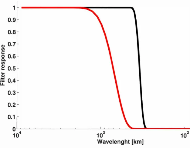
The low-pass filter is based on the discrete eosine transform (Denis et al., 2002a), with a graduai response function that attempts to mimic the spectrum of an equivalent 1.8°-mesh simulation. The lower and upper wavelength limits for the BB.15_Fl.8 are chosen to be 396 km and 1386 km, corresponding respectively to the l yquist length scale 2 D..x and to the smallest adequately resolved scales 7 D..x, as shown by Skamarock (2004) and Cholette et al. (2015); a cosine-squared function response is used between these two limits (as shown by the red line in Fig.l.3).
Two dynamical downscaling approaches will be compared using the BBE protocol: th ingle and double nesting, as shown on Fig.l.l.
12
1.3.1 Single nesting approach
The LB simulations using the single nesting follü\·V the usual BBE protocol as in (Denis et al., 2002b). In our case, the LB simulations were performed for four 1.5-month periods starting on November 15 (thus leaving out the initial 15 days as spin-up of the BB.15 simulations), for the years 1997 to 2000, using the BBF dataset as IC and LBC at 6 h intervals. The LB simulations were performed over five different domain sizes: 460 x 460, 260 x 260, 160 x 160, 110 x 110 and 60 x 60 grid points, respectively (Fig.1.2). The climate statistics of the LB were compared to those of the BB for the four months of December (thus leaving out the initial 15 days as spin-up of the LB simulations) over a common area of 44 x 44 grid points indicated by the dashed black square in Fig.l.2.
1.3.2 Double nesting approach
While the single nesting follows the standard BBE procedure, the design of the dou ble-nesting experiment deserves special attention. The challenge is to maintain the pe rfect-prognosis at tri bute of the BBE while designing a double-nesting strategy that normally involves the use of an intermediate-resolution simulation. After considering severa! alternatives, the following procedure was adopted. A surrogate to an intermediate -resolution simulation on a 0.45° mesh has been generated using a 0.15°-mesh simulation performed over a moderately large domain, and then using specifie filters to replicate the spectral characteristics and behaviour of a 0.45°-mesh simulation over an optimal domain size. The resulting simulation data will be referred to as Step Brother (SB.45). The Appendix details the procedure followed to determine the optimal conditions so that the SB.45 dataset represents a good proxy to an idealized 0.45°-mesh simulation while maintaining the perfect-prognosis approach using 0.15°-mesh LB simulations.
The SB.45 dataset corresponds to the first stage of the double nesting procedure in Fig.l.l. In turn, this SB.45 dataset serves to drive a 0.15°-mesh LB simulations for the second stage of double nes ting. Severa! 0.15°-mesh LB simulations were performed on various domain sizes (260 x 260, 160 x 160, 110 x 110 and 60 x 60 grid points, respectively), using a nesting interval of 1 h.
1.4 Analysis tools
A proper evaluation of high-resolution nested RCM simulations requires separating the large scales that are present in the driving LBC from the smaller scales that are only
13
resolved by the finer mesh of the RCM. The black line in Fig.l.3 show· the response of the analysis filter used to isolate the large-scale component: wavelengths longer than 400 km are retained entirely and those smaller than 300 km are removed, with a graduai
cosin -squared function transition in between. The small-scale component is obtained by ubtracting the large-scale component from the original fields. In particular, large cale refer to those scale present in the driving data and small scales correspond to those ab ent in the driving data. It is important to note that the analysis filter has been applied on a common area for all simulations, irrespective of the imulation domains.
Temporal decomposition of each variables \[1 is applied befor analysis. Any vari-able (w(x,t)) function of space x and time t will be split to analyze their time mean (also called stationary component) and time deviation (also called transient-eddy com-ponent), as follows
w(x, t) = w(x)
+
w'(x, t) (1.1)where • is the temporal mean and ' the time deviation. The transient-eddy variance is obtained as
(1.2)
The LB and BB statistics will be compared in terms of the ratio of their tra nsient-eddy standard deviation
r'
=O'~
s
(x)
1 ( -) , 0'88 X
(1.3)
the transient-eddy correlation
(1.4)
and the transient-eddy root mean square (RMS) difference
(1.5)
14
w(x)
=
(w(x))+
w*(x), ( 1.6) where () and * refer, respectively, to the spatial average and the spatial deviation of the field; the spatial-eddy variance is defined as( 1. 7)
The LB and BB statistics can be compared in terms of the ratio of spatial standard deviation as
r
*
= a[s * ) aBE ( 1.8) the spatial correlation as (1.9)and the RMS difference of spatial deviation as
(1.10)
The Taylor diagrams (Taylor, 2001) are useful to summarise succinctly the spatial
and temporal behaviours of the LBs compared to the BB.15_Fl.8. On the presentee! diagrams, the RMS are normalized by the standard deviation of the BB.
1.5 Results
In this section, selected variables are presentee! to give a representative picture of the
general behaviour of the spatial and temporal properties.
1.5.1 Stationary component
The large-scale stationary component of the simulations has bcen investigated. Figure
1.4 shows the Tay lor cliagrams for the large-scale stationary com panent of both the