HAL Id: tel-00821629
https://tel.archives-ouvertes.fr/tel-00821629
Submitted on 11 May 2013
HAL is a multi-disciplinary open access
archive for the deposit and dissemination of sci-entific research documents, whether they are pub-lished or not. The documents may come from teaching and research institutions in France or abroad, or from public or private research centers.
L’archive ouverte pluridisciplinaire HAL, est destinée au dépôt et à la diffusion de documents scientifiques de niveau recherche, publiés ou non, émanant des établissements d’enseignement et de recherche français ou étrangers, des laboratoires publics ou privés.
UNIVERSIT´
E DE NANTES
FACULT´E DES SCIENCES ET DES TECHNIQUES ´
ECOLE DOCTORALE 3MPL Ann´ee 2012
Correlated background and impact
on the measurement of ✓
13
with the
Double Chooz detector
TH`
ESE DE DOCTORAT
Discipline: Constituants ´el´ementaires et physique th´eorique Sp´ecialit´e: Physique des particules
Pr´esent´ee
et soutenue publiquement par
ALBERTO REMOTO
Le 5 Octobre 2012, devant le jury ci-dessousRapporteurs Dario AUTIERO Directeur de Recherche, IPN (Lyon) Achim STAHL Professeur, RWTH (Aachen)
Examinateurs Thierry GOUSSET Professeur, Subatech (Nantes)
Dominique DUCHESNEAU, Directeur de Recherche, LAPP (Annecy) Herv´e DE KERRET, Directeur de Recherche, APC (Paris) Directeur de th`ese Jacques MARTINO, Directeur de l’IN2P3, Subatech (Nantes) Encadrant de th`ese Anatael CABRERA, Charg´e de Recherche, APC (Paris)
The chances of finding out what’s really going on in the universe are so remote, the only thing to do is hang the sense of it and keep yourself occupied... The Hitchhiker’s Guide to the Galaxy, Douglas Adams
Abstract
The Double Chooz experiment uses antineutrinos emitted from the Chooz nuclear power plant (France) to measure the oscillation mixing parameter ✓13. A rate and shape analysis are performed to search for distortion in the measured energy spectrum due to ¯⌫e disappearance. The best fit value for the neutrino mixing parameter sin2(2✓13) is 0.109±0.030(stat.)±0.025(syst.). The precision and accuracy of the measurement relies on precise knowledge of the rates and spectral shapes of the backgrounds contaminating the ¯⌫e selection over the neutrino oscillation expected region.
This thesis studies the correlated background induced by muons interact-ing in the detector or in its surroundinteract-ings. The optimisation of the signal selection allow to reduce the correlated background < 0.2 % by tagging muons crossing the detector with efficiency > 99.999 % and applying a veto time of 1 ms upon a tagged muon. The remaining correlated background, arising from muons which either missed the detector or deposit an energy low enough to escape the muon tagging, has been estimated. For the first time, a pure sample of correlated background is studied in the energy region dominated by ¯⌫e, defining dedicated tagging strategies based the direct de-tection of background events by the outer-most detectors of Double Chooz: the ”inner-veto” and the ”outer-veto” detectors.
The correlated background measurement presented in this thesis concludes that the spectral shape is consistent with a linear correlated background spectral shape and a total rate of 0.60± 0.20 day 1. This represents the official Double Chooz results on correlated background, published in [20].
sant dans le d´etecteur ou dans ses environs. L’optimisation de la s´election du signal permet de r´eduire le bruit de fond corr´el´e < 0.2 % , d’une part en rep´erant les muons traversant le d´etecteur avec une efficacit´e > 99.999 % et d’autre part en appliquant un temps de latence apr`es une d´etection muon de 1 ms . Le bruit de fond corr´el´e restant dans notre ´echantillon de can-didats neutrinos, d´ecoulant de muons qui n’ont pas travers´e le d´etecteur ou d’un d´epˆot d’ ´energie des muons dans le d´etecteur en dessous du seuil d’identification, a ´et´e estim´e. Pour la premi`ere fois, un ´echantillon pur de bruit de fond corr´el´e est ´etudi´e dans la r´egion en ´energie domin´ee par les ¯⌫e , en d´efinissant des strat´egies de marquage d´edi´ees bas´ees sur la d´etection directe du bruit de fond par les d´etecteurs externes de Double Chooz: l’ ”inner-veto” et l’ ”outer-veto”.
La mesure du bruit de fond corr´el´e pr´esent´ee dans cette th`ese conclut que la forme spectrale est compatible avec une forme linaire pour le bruit de fond corr´el´e et un taux de comptage global de 0.60± 0.20 day 1. Ce chi↵re repr´esente dor´enavant le r´esultat officiel de Double Chooz en mati`ere de bruit de fond corr´el´ee, publi´e dans [20].
Acknowledgments
Since so many people contributed to this work over the last three years, it is not an easy job to thank them all as they deserve, but it’s worth a try. In a first place I would like to thank my supervisors, Dr. Anatael Cabr-era and Dr. Frederic Yermia. This work would have been simply impossible without their guidance. There are no words to express all my gratitude. Even if, strictly speaking, we have never worked together, I would like to thank Prof. Herv´e de Kerret and Prof. Jacques Martino to have super-vised my work from the top of their knowledge of high energy experimental physics.
I would also like to thank Prof. Achim Stahl, Prof. Dario Autiero, Prof. Dominique Duchesneau and Prof. Thierry Gousset for the important feed-back they provided by reading this manuscript in a critical way and being part to the jury.
I’m grateful to the whole ERDRE group at Subatech (Nantes) and to the whole Neutrino group at APC (Paris) where I had the honor to work with so many pleasant and talented physicists. In particular, I would like to explic-itly thank some of them. Dr. Muriel Fallot who at the beginning welcomed me in to the ERDRE group and for the fruitful discussions regarding the simulation of the expected ¯⌫e spectra. Dr. Arnaud Guertin for welcoming me in to his office and for his help with the sometimes excessive laboratory policies. Dr. Amanda Porta, Dr. Luca Scotto Lavina and Dr. Diego Stocco for making me feel like at home in Nantes. Prof. Alessandra Tonazzo for all the help she provided during my stay in Paris and for the email exchange in the spring 2009 from which all this started. Dr. Michel Obolensky for his great experience and knowledge kindly shared with me and all his help in the most difficult times. Dr. Jaime Dawson for the contagious enthusiasms she always puts in to work and for the time she dedicated to review this manuscript. Dr. Didier Kryn and Dr. Davide Franco for the always fruitful discussions and priceless advice about physics, electronics, computing and the nice dinners at their places. To whom I shared the hard life of a Ph.D. student, Tarek Akiri at the beginning, Anthony Onillon, Romain Roncin and Guillaume Pronost at the end.
I wish also to thank all my collaborators who make the Double Chooz ex-periment a pleasant and challenging working environment, which motivated me to do my best. In particular I’m grateful to Prof. Ines Gil Bottella and the Double Chooz CIEMAT members who welcomed me during many visits to Madrid, to Prof. Masahiro Kuze and the Kuze Lab members for the nice
available to discuss the mystery of our o✏ine code and share his experience, also beyond the work life. I will miss to work with you buddies.
Agli amici che ho avuto la fortuna di incontrare a Parigi. . . la mia famiglia all’estero. Pietro, che mi ha prestato la sua camera senza neanche conoscermi ed `e diventato poi un ottimo amico. Sempre disponibile per una birra, quat-tro chiacchiere e cose pazze tipo i film di Bud Spencer o la nostra dieta a base di fagioli e cipolle. Martino, il miglior compagno di scalate che avrei potuto incontrare. Importanti le nostre discussioni sulla sfera femminile (TT), il suo buon gusto per il cibo e gli alcolici hanno sempre reso indimenticabili le nostre cene (a seconda della quantit`a di vino). Franceschina, per le infinite chiacchiere, i calamari ripieni e la nostra prima ed imbarazzante mattina in rue d’Avron. Michela, la pi`u divertente e piacevole persona con cui ho condiviso l’ufficio, sempre in grado di capire cosa c’era di sbagliato, e non solo nel lavoro. Grazi anche ad Aurora, Claudio, Davide Federica, Filippo, Nicolais, Samir e Teresa.
Agli amici di una vita, Cisco, Fra, Giova, Greg, Loris e Marcos. Per farmi sentire,ogni volta che torno a Torino, come se non fossi mai partito. Ora so che sar`a sempre cos`ı.
Alla mia famiglia, Mamma, Pap`a, Nonna, Federico, Andrea, Barbara, Beat-rice & Leonardo sempre vicini ogni giorno, anche a centinaia di km di dis-tanza.
Ed in fine alla persona pi`u importante di tutte, Stefania, che mi ha ac-colto in casa sua e poi non siamo pi`u riusciti a fare a meno l’uno dell’altra. Grazie per essere stata e continuare ad essere sempre presente.
Contents
1 Introduction 13
2 Neutrino physics 17
2.1 The standard model of particle physics, an overview . . . 17
2.2 Neutrino history in brief . . . 19
2.3 Neutrino oscillation, the theory . . . 21
2.4 Measuring neutrino oscillation parameters . . . 23
2.4.1 Experimental determination of m212 and ✓12 . . . 24
2.4.2 Experimental determination of m2 23 and ✓23 . . . 27
2.4.3 Experimental determination of ✓13 . . . 31
2.4.4 Neutrino anomalies . . . 33
2.5 The problem with the neutrino mass . . . 35
2.6 Summary and open questions . . . 37
3 The Double Chooz experiment 41 3.1 The Double Chooz detector . . . 43
3.1.1 Target . . . 46 3.1.2 Gamma Catcher . . . 47 3.1.3 Bu↵er . . . 47 3.1.4 Inner Veto . . . 47 3.1.5 Shielding . . . 48 3.1.6 Outer Veto . . . 49
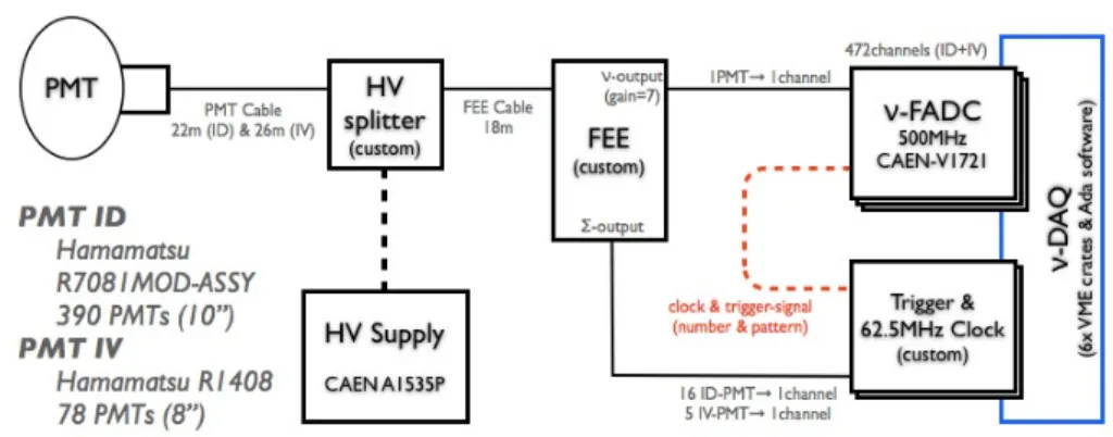
3.2 The detector read-out . . . 50
3.2.1 PMT and HV . . . 50
3.2.2 FEE . . . 51
3.2.3 FADC . . . 51
3.2.4 Trigger system . . . 52
3.2.5 OV read-out . . . 53
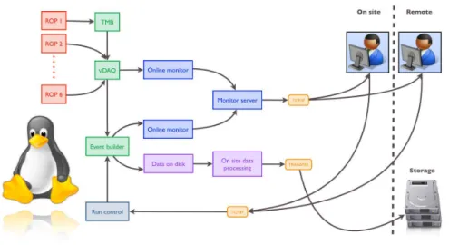
3.3 The online system . . . 53
3.3.1 Data acquisition . . . 54
3.3.2 Run control . . . 54
3.3.3 Onsite data handling . . . 55
3.3.4 Monitoring system . . . 57 9
3.5.7 Bugey4 normalisation and errors . . . 65
3.6 Detector simulation . . . 68
3.7 Read-out system simulation . . . 68
3.8 Data reconstruction . . . 69
3.8.1 Pulse reconstruction . . . 70
3.8.2 Vertex reconstruction . . . 71
3.8.3 Muon tagging and track reconstruction . . . 72
3.8.4 Energy reconstruction . . . 74
3.9 Conclusions . . . 77
4 Measurement of ✓13 with the Double Chooz far detector 79 4.1 Data sample . . . 79
4.1.1 External trigger . . . 80
4.1.2 Instrumental noise . . . 80
4.1.3 Muon correlated events . . . 81
4.2 ⌫¯e signal selection . . . 82
4.2.1 Selection cuts summary . . . 86
4.3 Backgrounds . . . 88
4.3.1 Accidental background . . . 88
4.3.2 Cosmogenic radioisotopes background . . . 89
4.3.3 Correlated background . . . 91
4.3.4 Background summary . . . 92
4.4 Selection efficiencies and systematics . . . 93
4.4.1 Trigger efficiency . . . 93
4.4.2 Neutron detection efficiency . . . 93
4.4.3 Spill-in/out . . . 99
4.5 Data analysis summary . . . 99
4.6 Final fit and measurement of ✓13 . . . 99
4.7 Summary and Conclusions . . . 105
5 Correlated background 107 5.0.1 Fast Neutrons . . . 107
5.0.2 Stopping Muon . . . 108
CONTENTS 11
5.1.1 MC technique . . . 109
5.1.2 Tagging techniques . . . 109
5.2 High energy analysis . . . 111
5.3 OV Tag analysis . . . 115
5.4 Fast Neutrons analysis . . . 117
5.4.1 IV Tagging . . . 119
5.4.2 IVT background . . . 123
5.4.3 IVT summary . . . 131
5.4.4 Fast Neutron shape and rate . . . 134
5.4.5 Systematics uncertainty on the IVT threshold . . . 136
5.5 Stopping Muon analysis . . . 138
5.5.1 High energy light noise . . . 139
5.5.2 Stopping Muon shape and rate . . . 143
5.5.3 Validating high energy light noise rejection . . . 145
5.5.4 Validating high energy delayed window . . . 149
5.6 Estimation of correlated background for ✓13 measurement . . 151
5.6.1 Reducing the correlated background with the OV veto 153 5.6.2 Correlated background shape and uncertainty for the final fit . . . 154
5.7 Conclusion . . . 157
6 Conclusions 159
7 Contributions to Double Chooz 163
List of figures 166
List of tables 179
Chapter 1
Introduction
The Standard Model has been widely confirmed by many experiments to be the theory regulating the interactions among subatomic particles. How-ever, some modifications were introduced in order to explain the peculiar behaviour of the neutrino. For this reason, neutrino physics is one of the most important branches of modern particle physics. Among the di↵erent interesting aspects regarding the neutrinos, one of the most fascinating phe-nomena is the so-called neutrino oscillation.
Since the late 1960s several experiments observed discrepancies between the number of neutrinos coming from the Sun and the theoretical prediction. Similar discrepancies were found observing neutrinos produced in the top of the Earth atmosphere. These discrepancies, known as the solar and atmo-spheric neutrino anomalies respectively, remained unsolved for about thirty years until being recently understood in terms of the oscillation mechanism. Neutrino oscillation was postulated by Pontecorvo in 1957 in analogy with the K0 $ K0oscillations. When the second neutrino family was discovered, Maki, Nakagawa and Sakata proposed in 1962 the possibility of oscillation among the neutrino families, introducing the concept of lepton flavour mix-ing.
In analogy with the mixing in the quark sector, the lepton flavour mixing implies that the weak eigenstates can be regarded as superpositions of mass eigenstates. The mass eigenstates travel at di↵erent speeds in the vacuum, causing di↵erent propagation phases and resulting in an oscillation among the flavour eigenstates. Such oscillation requires neutrinos to be massive particles, with a non degenerate mass spectra.
The observation of neutrino oscillation implies a modification in the Stan-dard Model, in order to account for flavour mixing in the lepton sector and massive neutrinos, opening the possibility to explore new physics.
The mixing is mathematically described by the so-called mixing matrix, de-pending from 3 mixing angles and a complex phase whose values have to be measured experimentally. The solar and atmospheric experiments
13 e
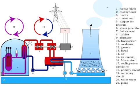
chain reaction produced in the Chooz nuclear power plant (France). The value of ✓13is inferred by a rate and shape analysis to search for a distortion in the measured energy spectrum due to ¯⌫e disappearance.
In order to reduce the systematic uncertainties related to the ¯⌫e detection and to the knowledge of the un-oscillated ¯⌫espectra produced by the reactor core, two functional identical detectors are employed to perform a relative measurement.
The far detector is installed in the laboratory hall previously used by the CHOOZ experiment, located at a mean distance of 1050 m from the two re-actor cores, near the first oscillation minimum due to ✓13. The near detector will be placed at a mean distance of 400 m from the reactor cores, where oscillation e↵ects due to ✓13 are expected to be negligible.
The detector design consists of a 10.3 m3 of liquid scintillator target, sur-rounded by passive and active veto volumes. The ¯⌫e are detected through the inverse -decay reaction in liquid scintillator. The signal consists in a coincidence between a prompt event, produced by the positron with an en-ergy related to the ¯⌫e energy, and a delayed event, produced by the neutron capture. The signal signature is improved by doping the target scintillator with gadolinium since it provides a better energy signature for the delayed event, with the emission of ⇠ 8 MeV rays, and speeds up the neutron capture process with respect to the H of the liquid scintillator. The detector design, has been optimised to reduce the background contamination. The far detector was build between 2009 and 2010 and began data taking in April 2011. The near laboratory hall construction will finish by the end of 2012 and the near detector is expected to start data taking by the end of 2013. In this first phase with the far detector only, the simulation of the reactor ¯⌫e flux is required to perform the oscillation analysis.
The detailed description of the Double Chooz experiment is presented in Chapter 3, highlighting the major improvements with respect to the previ-ous CHOOZ experiment.
The measurement of ✓13 has been recently performed by analysing far de-tector data, taken from 13th April 2011 to 30th March 2012. A rate and shape analysis has been performed by comparing the ¯⌫e energy spectrum
15 measured at the far detector with the expected un-oscillated spectrum from the simulation of the reactor ¯⌫e flux. A shape consistent with ✓13 related oscillation has been observed. The analysis is described in Chapter 4 high-lighting the improvements obtained with respect to the first Double Chooz result.
The precision and accuracy of the measurement relies on precise knowledge of the rates and spectral shapes of the backgrounds contaminating the ¯⌫e selection over the neutrino oscillation expected region. For this reason most of the e↵ort have been focused on the estimation of the background, which is due to three main sources: natural radioactivity, cosmogenic radio isotopes and correlated background.
This thesis studies the correlated background produced by cosmic muons interacting in the detector or in its surrounding, whose prompt and delayed events come from the same physical process. The correlated background contamination is strongly reduced by adding dedicated cuts to the ¯⌫e se-lection. The remaining background contamination and its spectral shape are estimated by a dedicated analysis developed in Chapter 5. For the first time, a pure sample of correlated background is studied in the energy re-gion dominated by ¯⌫e , defining dedicated tagging strategies based on the direct detection of background events by the outer-most detectors of Double Chooz: the ”inner-veto” and the ”outer-veto” detectors.
The results obtained in this thesis are summarised in Chapter 6 with possi-ble improvements and further development, which could be foreseen for the future.
Finally, Chapter 7 briefly summarises the results and contributions achieved during the development the present thesis.
Chapter 2
Neutrino physics
In this chapter the physics related to the neutrino is widely discussed both from the theoretical and experimental point of view, with a particular focus on neutrino oscillation. The current state of the art regarding the measure-ment of the oscillation parameters is given with a description of the most important experiments in this field. The problem related to the nature of the neutrino mass is also briefly described. Finally, the open questions and the future e↵orts to be addressed by the neutrino community are also discussed.
2.1
The standard model of particle physics, an
overview
The Standard Model of particle physics (SM) is the theory describing how the fundamental constituents of our universe interact.
From the technical point of view theSM is a renormalisable gauge field the-ory, based on the symmetry group SU (3)C⌦SU(2)L⌦U(1)Y which describe strong, weak and electromagnetic interaction, via the exchange of spin-1 gauge field: eight massless gluons for the strong interaction, one massless photon for the electromagnetic interaction and three massive bosons, W± and Z0 for the weak interaction.
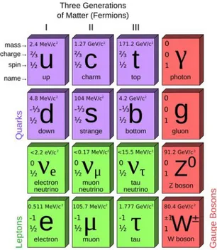
The known elementary particles and antiparticles are fermions with spin-1/2 and are organised in two families according on how they interact: quarks and leptons. Quarks interacts with all the three forces, while leptons in-teract only through the electromagnetic and/or the weak force. Quarks and leptons exist in three generations or flavours, with di↵erent masses and flavour quantum numbers, but with identical interactions, which make the SM symmetric with respect to the flavour. A summary of SM fermions and bosons is shown Fig. 2.1.
The fermions are a representation of the symmetry group and can be written 17
Figure 2.1: The Standard Model of elementary particles (antiparticles are not show for brevity), with the gauge bosons in the rightmost column.
Due to the gauge symmetry of the theory, particles are so far massless. While such assumption appears as a good approximation at high energies (E MZ, MW), where the weak and electromagnetic interactions have similar strengths and are described by the unique electroweak force, at low energies the mass of the W± and Z bosons make the weak interaction weaker than the electromagnetic interaction.
The weak gauge bosons masses are acquired by introducing a new scalar field and breaking the gauge symmetry by choosing an expectation value for its vacuum state. This mechanism, known as spontaneous symmetry breaking, generates the masses for the weak bosons and give rise to the appearance of the spin-0 Higgs boson. The photon and the gluons remain, by construction, massless particles in agreement with experimental observations.
2.2 Neutrino history in brief 19 mass term through the so called Higgs mechanism which couples the right-handed singlets with the left-right-handed doublets via the Yukawa coupling con-stant, providing masses of the form of:
LY = mllLlR+ mqqLqR+ h.c. (2.2) where the mass term for the fermions (as example) is given by ml:
ml= v p
2 l (2.3)
where v is the vacuum expectation value of the Higgs field and i is the Yukawa coupling constant, that assumes di↵erent values for the di↵erent fermions. To explain the observed masses, i varies from ⇠1 for the heav-iest fermion, the quark top, to ⇠10 5 for the lighter charged fermion, the electron.
Since the observed neutrinos are only left-handed, they are not allowed to acquire mass though the Higgs mechanism, remaining massless in the SM. The SM provides a beautiful theoretical model which is able to accommo-date most of the present knowledge on electroweak and strong interactions. It is able to explain many experimental facts and, in some cases, it has suc-cessfully passed very precise tests. Even the long search for the Higgs boson has recently provided conclusive evidence for the discovery of a new particle, consistent with theSM Higgs boson hypothesis [11].
In spite of the impressive phenomenological success, the SM leaves many unanswered questions to be considered as a complete description of the fun-damental forces. There is no understanding regarding the existence of three (and only three) fermions families as well as their origins. There is no an-swer to the observed mass spectrum and mixing pattern. These, and others questions remain open and require new physics beyond the SM. As will be stressed in the rest of this chapter, first hint from such new physics has emerged with evidence of neutrino oscillations.
2.2
Neutrino history in brief
The neutrino was postulated by Pauli in 1930 as an e↵ort to explain the con-tinuous electron energy spectrum observed in nuclear decays [82]. Pauli proposed a new particle, electrically neutral to conserve charge, with spin 1/2 to conserve angular momentum, weakly interacting since it was not de-tected at that time and with a mass lighter than the electron. Following the discovery of the neutron by Chadwick in 1932 , Fermi explained theoreti-cally the -decay [58] as the decay of a neutron in proton, electron and a neutrino:
The neutron is captured by the Cadmium giving further gamma rays with a delay of about 5 µs.
The second neutrino family was discovered in 1962 at Brookhaven National Laboratory [48]. A spark chamber detector was exposed to the first neu-trino beam created by the decay of pions. Neuneu-trinos were observed to create muons through charged current interaction in the detector, suggesting such neutrinos were of a di↵erent species with respect to the one observed by Cowan and Reines.
When in 1975 the third family charged lepton, the ⌧ , was discovered [83], it was postulated that a third type of neutrino, ⌫⌧, would have to exist. The tau neutrino was finally directly observed in 2001 by the DONUT experi-ment at Fermilab [55].
The CERN experiments at LEP during the 1990s studied in detail the prop-erty of the W± and Z bosons. The number of active neutrinos was precisely constrained to three families by measuring the Z decay width [10], which depends from the number of kinematically accessible decay channels:
N⌫ = SMinv ⌫
= 2.9840± 0.0082 (2.6) where inv is the total Z with minus the measured individual contribution from charged fermions and SM⌫ is the theoretical contribution of one neu-trino flavour. It should be noted that the LEP measurement constrains only the numbers of active neutrinos, the ones for which the decay Z ! ⌫x⌫x is kinematically allowed. The existence of a fourth sterile neutrino family with masses bigger than mZ/2' 45.5 GeV is not excluded.
Within these experimental evidences, neutrinos are coupled with corre-sponding leptons in a flavour doublet and SM interactions conserve the lepton flavour quantum number (i.e. charged-current interactions transform the ⌫l (⌫l) into the corresponding charged lepton l (antilepton l+)). Nevertheless, since the late 1960s several experiments observed some discrep-ancies between the number of neutrinos coming from the sun and the theo-retical prediction. Such discrepancies known as the solar neutrino anoma-lies remained unsolved for about thirty years until being later understood
2.3 Neutrino oscillation, the theory 21 in terms of the so called neutrino oscillation mechanism. As explained with more details in the following sections, the oscillation mechanism requires the neutrino to have non-null mass and lepton flavour quantum numbers are no longer conserved.
The SM is clearly not complete and requires extension to accommodate neutrino oscillation mechanism and its consequences.
2.3
Neutrino oscillation, the theory
Neutrino oscillation were postulated in 1957 by Pontecorvo [86]. In analogy with K0$ K0oscillations, Pontecorvo suggested the possibility of neutrino-antineutrino oscillation ⌫ $ ⌫. When the second neutrino family where discovered, Maki, Nakagawa and Sakata proposed in 1962 the possibility of oscillation among the neutrino families introducing the concept of lepton flavour mixing [101]. The neutrino oscillation mechanism is based on the fact that if neutrino have a non-null mass, flavour states|⌫↵i (interaction states) and mass states |⌫ii (propagation states) could not coincide, in analogy to the mixing in the quark sector:
|⌫↵i = X
i
U↵,i⇤ |⌫ii (2.7) where ↵ represent the flavour families (e, µ, ⌧ ),|⌫ii the mass states of mass mi (with i = 1, 2, 3) and U is the so called PMNS1 unitary mixing matrix. Neutrinos are produced via weak interaction in a defined flavour eigenstate |⌫↵i together with the corresponding lepton ↵. Assuming the neutrino is produced at time t = 0:
|⌫(t = 0; L = 0)i = |⌫↵i = X
i
U↵,i⇤ |⌫ii (2.8) and propagates as a free particle following the Schrodinger equation, after a time t: |⌫↵(t, L)i = X i U↵,i⇤ e i(Eit pL)|⌫ ii (2.9)
assuming the three mass eigenstates propagate with the same momentum with relativistic energies (p' E m):
Ei = q p2+ m2 i ' p + m2i 2p ' E + m2i 2E (2.10)
Eq. 2.9 could be written, using natural units (c =~ = 1), as: |⌫↵(t, L)i =
X i
U↵,i⇤ e im22EiL|⌫ii (2.11) 1Pontecorvo-Maki-Nakagawa-Sakata matrix
a neutrino created with flavour ↵, at L = 0, with a di↵erent flavour , after a distance L, is obtained from Eq. 2.11:
P (⌫↵! ⌫ ) = |h⌫ |⌫↵(L)i|2 = X i U↵,i⇤ U ,ie i mi 2EL 2 (2.13) = X i |U↵,iU⇤,i|2+ 2Re 0 @X i>j U↵,iU⇤,iU↵,j⇤ U ,je i m2ij 2E L 1 A
An oscillation term appears as a function of the distance between the neu-trino creation point (source) and the detection point (detector), and the neutrino energy. The oscillation frequency is proportional to the squared di↵erence between the mass states m2ij = m2j m2i while the oscillation amplitude is proportional to the PMNS matrix elements U↵,i.
The PMNS mixing matrix have a complicated form: U = 0 @ c12c13 s12c13 s13e i s12c23 c12s23s13ei c12c23 s12s23s13ei s23c13 s12c23 c12c23s13ei c12s23 s12c23s13ei c23c13 1 A (2.14)
where cij = cos ✓ij and sij = sin ✓ij. The angles ✓12, ✓13, ✓23 represent the mixing angles and is a CP violation phase. Two additional phases have to be taken into account if neutrinos are Majorana particles but such phases do not impact the neutrino oscillation.
As shown in Eq. 2.13, neutrino oscillation depends also from the mass squared di↵erences between mass states: m2
12, m223 and m231 which only two of them are independent because related through:
m212+ m223+ m231= 0 (2.15) Consequently neutrino oscillation depends on 6 free parameters: 3 mixing angles, 2 mass squared di↵erences and one complex CP violation phase. For practical reasons, the mixing matrix is usually factorized in terms of
2.4 Measuring neutrino oscillation parameters 23 three matrices M2,3⇥ M1,3⇥ M1,2: U = 0 @ 1 0 0 0 c23 s23 0 s23 c23 1 A 0 @ c13 0 s13e i 0 1 0 s13e i 0 c13 1 A 0 @ c12 s12 0 s12 c12 0 0 0 1 1 A (2.16) M2,3 is parametrized in terms of ✓23 which is the mixing angle dominating the ⌫µ ! ⌫⌧, related to the oscillation of atmospheric neutrino. M1,2 is parametrized in terms of ✓12 dominating the transition ⌫e ! ⌫µ,⌧, related to the oscillation of neutrino coming from the sun. Finally, M13 depends on ✓13 which is the mixing matrix dominating the oscillation ⌫µ! ⌫e. The CP phase always appears multiplied by the terms sin ✓13, so it would be measurable only if ✓13 is di↵erent than zero.
To conclude, the observation of the neutrino oscillations has two main con-sequences: neutrinos have a non-zero mass and the lepton flavour is not conserved.
2.4
Measuring neutrino oscillation parameters
To easily understand neutrino oscillation experimental results, the simpler case with only two active neutrino is considered. The mixing among two neutrino families can be described by a real and orthogonal 2⇥ 2 matrix with one mixing parameter, the rotation angle ✓ between the flavour and the mass eigenstates:
✓ ⌫↵ ⌫ ◆ = ✓ cos ✓ sin ✓ sin ✓ cos ✓ ◆ ✓ ⌫1 ⌫2 ◆ (2.17) The oscillation probability take the form:
P (⌫↵! ⌫ ) = sin2(2✓) sin2 ✓ m2L 4E ◆ (2.18) the amplitude of the oscillation, sin22✓, is determined by the mixing angle ✓ and does not allow to distinguish between ✓ and ⇡/2 ✓, which are not physically equivalent.
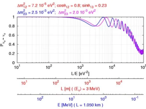
Restoring the physics units, the oscillation phase becomes: = 1.27 ✓ m2(eV2)L(km) E(GeV ) ◆ (2.19) In the limit where ⌧ 1, P (⌫↵ ! ⌫ ) ' sin22✓( m2L/(4E))2, so the measurement of the oscillation probability would determine information only on the product sin2(2✓)⇥ m2. The oscillation would not have enough time to develop and the number of neutrino oscillation events measured in the
' 1.
Even if three neutrino families exist, the mixing parameters are such that the dominant oscillation pattern is driven by the two flavour mixing, while the third flavour contribute at the second or higher order. For this reason the results of oscillation experiments are often shown in a two neutrino scenario and determine a single mixing angle and squared mass di↵erence.
2.4.1 Experimental determination of m2
12 and ✓12
Measurement of m212 and ✓12 oscillation parameters has been performed by Super-Kamiokande (SK) and SNO using neutrino created in the ther-monuclear reaction produced in the sun. The same parameters has also been measured by KamLAND using terrestrial ¯⌫e emitted by nuclear power plant. Results from global analysis is shown in Fig. 2.2 [91].
Solar neutrinos
Solar neutrino are ⌫e coming from the process responsible for solar power production: 4p + 2e ! 4He + 2⌫e+ 26.7 MeV. The process take place through di↵erent reactions and consequently solar neutrino are characterised by di↵erent energy spectra as shown in Fig. 2.3 [39]. The typical neutrino flux reaching the earth is of about 108 ⌫/s/m2.
Several experiments measured the solar neutrino flux, starting with the pio-neering Chlorine experiment in the Homestake mine, proposed by Davis [50]. The ⌫e flux were measured in a tank of 400 m3 of C2Cl4 counting the num-ber of radioactive Ar nuclei produced by the inverse beta decay reaction 37Cl + ⌫
e ! Ar + e . Only one third of the neutrino flux predicted by the Standard Solar Model were measured. At that time an error on the experimental measurements or in the Standard Solar Model was assumed as possible explanation of the observed deficit. While error in the theoretical model were excluded by a better understanding of the sun, further exper-imental measurements, performed with di↵erent technique by Gallex [61], Sage/GNO [13] and Super Kamiokande [63] confirmed the deficit in the solar neutrino flux.
2.4 Measuring neutrino oscillation parameters 25
3-flavour oscillations
The dominanting oscillation modes
! 0.2 0.4 0.6 0.8
sin
2!
12 0 5 10 15"
m
2[ 10
21 -5eV
2]
solar neutrino exps.
KamLAND combined ★ 0 0.25 0.5 0.75 1
sin
2θ
23 1 2 3 4∆m
2[ 10
31 -3eV
2]
MINOS
atmospheric
global
sin
2
✓
12
0.3
sin
2
✓
23
0.5
m
2
21
m
2
31
1
30
T. Schwetz 9Figure 2.2: m212 and ✓12 parameters from global analysis of solar and reactor experiments [91].
Figure 2.3: Di↵erent processes contributing to the solar neutrino spec-trum [39].
tot e µ ⌧
The three di↵erent reactions measured three independent linear combina-tion of electron, muon and tau neutrino fluxes, as shown in Fig. 2.4. Such measurement allowed to obtain clear evidence of solar neutrino oscillation in term of ⌫e! ⌫e,µ,⌧, of which ⌫e is only one third of the total. Moreover, the total initial ⌫eflux has been determined independently from theoretical
model. DETERMINATION OF THE νeAND . . . . I DATA SET PHYSICAL REVIEW C 75, 045502 (2007)
0 1 2 3 4 5 6 0 1 2 3 4 5 6 7 8 ) -1 s -2 cm 6 (10 e φ ) -1 s -2 cm 6 (10τµ φ SNO NC φ SSM φ SNO CC φ SNO ES φ
FIG. 41. (Color) Flux of8B solar neutrinos that are µ or τ flavor
vs flux of electron neutrinos deduced from the three neutrino reactions in SNO. The diagonal bands show the total8B flux as predicted by
the BP2000 SSM [78] (dashed lines) and that measured with the NC reaction in SNO (solid band). The intercepts of these bands with the axes represent the ±1σ errors. The bands intersect at the fit values for φeand φµτ, indicating that the combined flux results are
consistent with neutrino flavor transformation with no distortion in the8B neutrino energy spectrum.
in interpreting these results. Although the signal-extraction fit has three free parameters, one should not subtract three degrees of freedom for each χ2, since the fit is a global fit to
all three distributions. Furthermore, the actual signal extraction is a fit to the three-dimensional data distribution, whereas the χ2s are calculated with the marginal distributions. These “χ2” values demonstrate that the weighted sum of the signal pdfs provides a good match to the marginal energy, radial, and angular distributions.
Figure 42 shows the marginal radial, angular, and energy distributions of the data along with Monte Carlo predictions for CC, ES and NC + background neutron events, scaled by the fit results.
2. Results of fitting for flavor content
An alternative approach to doing a null hypothesis test for neutrino flavor conversion, as discussed in Sec.VIII D, is to fit for the fluxes of νe and νµτ directly. This is a simple change
of variables to the standard signal extraction. Fitting for the
TABLE XXI. χ2 values between data
and fit for the energy, radial, and angular distributions, for the fit using the constraint that the effective kinetic energy spectrum results from an undistorted8B shape.
Distribution Number of bins χ2 Energy 42 34.58 Radius 30 39.28
Angle 30 19.85
-1.0 -0.5 0.0 0.5 1.0
Ev
ents per 0.05 wide bin
0 20 40 60 80 100 120 140 160 cos ES CC NC + bkgd neutrons Bkgd (a) 0.0 0.2 0.4 0.6 0.8 1.0 1.2 Ev
ents per 0.1 wide bin
0 100 200 300 400 500 CC NC + bkgd neutrons ES Bkgd Fiducial V olume (b) 3 R 5 6 7 8 9 10 11 12 13 Ev ents per 500 k eV 0 100 200 300 400 500 600 20 → NC + bkgd neutrons ES CC Bkgd (c) (MeV) eff T θ
FIG. 42. (Color) (a) Distribution of cos θ! for Rfit 6 550 cm.
(b) Distribution of the radial variable R3
= (Rfit/RAV)3. (c) Kinetic
energy for Rfit6 550 cm. Also shown are the Monte Carlo predictions
for CC, ES, and NC + background neutron events scaled to the fit results and the calculated spectrum of β-γ background (Bkgd) events. The dashed lines represent the summed components, and the bands show ±1σ statistical uncertainties from the signal-extraction fit. All distributions are for events with Teff > 5 MeV.
flavor content instead of the three signal fluxes, we find φ(νe) = 1.76 ± 0.05 × 106cm−2s−1,
φ(νµτ) = 3.41 ± 0.45 × 106cm−2s−1.
The statistical correlation coefficient between these values is −0.678. We will discuss the statistical significance of
045502-51 (km/MeV) e ! /E 0 L 20 30 40 50 60 70 80 90 100 Survival Probability 0 0.2 0.4 0.6 0.8 1 e ! Data - BG - Geo
Expectation based on osci. parameters determined by KamLAND
(a)
(b)
Fig. 7: Determination of the electron and muon/tau neutrino fluxes by SNO (a). Electron antineutrino survival probability at KamLAND (b).
the electron and the delayed coincidence with the signal from the neutron capture used to observe it.
The neutrino energy is directly related to the positron energy, E
⌫e= E
e++ m
nm
p, which allows to
measure the neutrino oscillation probability as a function of the energy and as a consequence i) to obtain
a good m
212
determination [
40
] and ii) to observe the oscillation pattern, including an oscillation dip,
in the survival probability, as shown in Fig.
7
b [
40
].
4.4 The unknown oscillation parameters
The mixing angle ✓
13has not been measured yet, but both direct and indirect bounds have been obtained
from the CHOOZ and Minos experiments, mentioned above, and from the analysis of subleading
ef-fects in the atmospheric and solar neutrino experiments. The result of a global fit on ✓
13are shown in
Fig.
8
a [
23
].
The determination of ✓
13is important for several reasons. It offers an handle on the origin of
the neutrino (and quark) masses and mixing angles. In particular, it allows to discriminate among
dif-ferent flavour models. And it is important for phenomenology, as it is crucial in the study of leptonic
CP-violation, supernova signals, and subleading effects, for example in ⌫
µ$ ⌫
⌧transitions at the m
223oscillation frequency. From the experimental point of view, a rich experimental program is available.
Several terrestrial experiments are running or have been planned using different techniques: conventional
beams obtained from pion decays, so called “beta-beams”, obtained from the beta decay of radio-active
ions circulating in a storage ring with long straight sections, and neutrino factory beams, obtained from
the decay of muons also circulating in a storage ring. A summary of the prospects on the ✓
13determi-nation are shown in Fig.
8
b for different values of the experimental parameters [
41
]. The figure uses the
GLoBES package [
42
,
43
]. References for the single experiments are shown in Figure.
Let us now discuss the determination of the sign of m
223
. I remind that this parameter determines
the pattern of neutrino masses, enters the analysis of supernova neutrino signals and of long baseline
terrestrial neutrino experiments, and determines the possibility to measure neutrinoless double beta decay
(see below). This parameter can be determined in the presence of matter effects. Let us consider the three
neutrino effective Hamiltonian for propagation in matter and let us take the m
212
= 0
limit for simplicity
18
Figure 2.4: Solar neutrino fluxes determined by SNO through elastic scat-tering (ES) neutral current (NC) and charged current (CC) interactions. The expected flux from the SSM is also shown and it is in agreement with the measured total flux [30].
Long baseline reactor neutrinos
The Kamioka Liquid-scintillator Anti-Neutrino Detector (KamLAND) ex-periment also played an important role in the determination of the solar oscillation parameters [16].
2.4 Measuring neutrino oscillation parameters 27 The neutrino energy is of the order of few MeV and the average distance between detector and reactors is of about 200 km. Given the mass squared di↵erence measured by solar experiments of⇠ 7.5⇥10 5eV2, the oscillation phase m212L/(4E) is of the order of 1, which provide the best condition for a precise measurement of the oscillation parameters.
The ¯⌫e detection is performed through charged current inverse beta decay reaction ⌫e+ p! e++ n in liquid scintillator. The positron and the delayed neutron capture on H gives a clean signature of ¯⌫einteraction. The ¯⌫eenergy is directly measured from the positron energy, E⌫e = Ee++ mn mp, giving
the possibility to measure the neutrino oscillation probability as a function of the energy.
A precise determination of m212 and the shape of the oscillation pattern are obtained as shown in Fig. 2.5.
Figure 2.5: Ratio of the background and geo-neutrino subtracted anti-neutrino spectrum to the expectation for no-oscillation as a function of L/E. L is the e↵ective baseline taken as a flux-weighted average (L=180km) [16].
2.4.2 Experimental determination of m2
23 and ✓23
The first measurement of m223and ✓23has been performed by SK using at-mospheric neutrinos. Further measurements have been performed to confirm SK results by K2K, MINOS and Opera using ⌫µ produced at accelerators. Results from global analysis are shown in Fig. 2.6 [91] and described in more details in the following sections.
Atmospheric neutrinos
Atmospheric neutrinos are produced by cosmic rays interacting in the high atmosphere producing mainly pions and kaons. The charged pions mainly
Figure 2.6: m223 and ✓23 parameters from global analysis of atmospheric and accelerator experiments [91].
decay though weak charged current ⇡± ! µ±⌫µ(⌫µ). The muons subse-quently decay as µ± ! e±⌫
e(⌫e) + ⌫µ(⌫µ) giving, as a first approximation two muon neutrinos for each electron neutrino.
Atmospheric neutrinos travel a distance between ⇠ 10 km (if coming from small zenith angles) and ⇠ 104 km (if coming from large zenith angles) as schematised in Fig. 2.7. Their energy spans from a few MeV up to sev-eral GeV. Since neutrinos can be generated at any point of the atmosphere, neutrinos of the same energy can travel very di↵erent distances before reach-ing the detector, givreach-ing di↵erent oscillation probabilities. Thus a detector able to distinguish muon neutrinos from electron neutrinos and also able to recognise their incoming direction is necessary.
SK is a large water Cherenkov detector located in the Kamioka mine (Japan) under 2.7 km of rock to shield the detector from cosmic rays. It con-tains about 50 ktons of water and it is surrounded by about 13000 PMTs. Neutrinos undergo charged current interaction producing charged leptons. The lepton is generally produced with ultra-relativistic energy and it is de-tected through the cone of Cherenkov light produced as it travels through the detector. The flavour of the lepton is identified by the shape of the Cherenkov ring. The position of the ring allows to determine the lepton directions, which is correlated to the neutrino direction for energies larger than⇠ 1 GeV. The lepton energy could also be obtained from the amount
2.4 Measuring neutrino oscillation parameters 29
have an average energy of 3 MeV. The results of CHOOZ ruled out from the possible
expla-nation of the atmospheric neutrino oscillation, described in the next section, the oscillation
⌫
e! ⌫
µand provided the limit ✓
13< 10 for
m
213= 3
· 10
3eV
2.
1.4.3
Atmospheric neutrino oscillations
After the Sun, the other main natural source of neutrinos is the earth atmosphere.
An intense flux of cosmic rays, primarily protons, arrives on the high atmosphere producing
a huge number of secondaries, in particular pions. These particles then decay in flight via
±
! µ
±+⌫
µ
(⌫
µ). The produced muons again decay according to µ
±! e
±+⌫
e(⌫
e)+⌫
µ(⌫
µ).
The typical energy spectrum of atmospheric neutrinos starts at about hundred MeV and
ex-tends up to several GeV.
Figure 1.7: Different flight distances, between their production point and SuperKamiokande,
for neutrinos produced in cosmic ray interactions with the Earth atmosphere.
The measurement of the atmospheric neutrino oscillation requires a different technique
from that used for solar neutrinos, mainly because the atmosphere cannot be considered
as a point-like source at fixed distance, like it was the case of the Sun. Neutrinos can be
generated at any point of the atmosphere, thus neutrinos of the same energy born at the
same time can travel very different distances before reaching the detector and this gives
different oscillation probabilities (see figure 1.7). To study the oscillation probability it is
19
Figure 2.7: Flight distance between the creation point and the SK detector for neutrinos created in atmosphere.
of light collected by the PMTs if the lepton stops into the detector. Even if the lepton energy is not strongly correlated to the neutrino energy it allows to handle the energy dependence of the oscillation probability.
SK provided in 1998 the first firm evidence of neutrino flavour transition comparing the expected number of events with the observed ones, as a func-tion of the zenith angle. SK observed that there are twice as many downward going ⌫µ than upward going ⌫µ, as shown in Fig. 2.8 [96]. The hypothesis that ⌫µ have interacted crossing the earth is not reliable because the earth is nearly transparent for neutrinos with energy of about few GeV and a similar behaviour should have also been found for ⌫e. Moreover, since no excess of the electron neutrino flux has been found, the observed oscillation is attributed to the transition ⌫µ! ⌫⌧.
Accelerator experiments
Experiments using neutrino produced at accelerator have also been per-formed to confirm the results obtained by SK.
The K2K experiment in Japan used ⌫µ produced from a pulsed beam at KEK and the SK detector placed at about 250 km. The average neutrino energy is slightly above 1 GeV. Given the mass squared di↵erence of about 2.5⇥ 10 3 eV2 measured with atmospheric neutrino by SK, the oscillation
Figure 1.8: SuperKamiokande results[24]. The neutrino fluxes are measured in bins of the zenith angle ✓ and divided in two categories, muon events created by a ⌫µ interaction, and electron events, created by a ⌫e interaction. A further division is done according to the energy of the lepton.
The larger detector of this type is SuperKamiokande[24], a 50 kton water Cerenkov de-tector. In addition to the solar neutrinos SuperKamiokande observes atmospheric neutrinos, separating the neutrino flux for different directions (see figure 1.8). The experiment counts ⌫e and ⌫µ in bins of the zenith angle ✓ (cos ✓ = 1 for the neutrinos coming from the zenith and cos ✓ = 1 if they come from the nadir). The experimental result, first presented in
20
Figure 2.8: The ⌫e and ⌫µ fluxes are measured as a function of the zenith angle and divided with respect to the lepton energy. Black points represent data, green histogram represent MC expectation with oscillation hypothesis and red histogram represent MC expectation in case of no oscillations [96].
phase is of the order of 1, which represent the best condition to measure oscillation.
The oscillation parameters are measured through ⌫µdisappearance, P (⌫µ! ⌫µ) = 1 P (⌫µ ! ⌫x), comparing the ⌫µ flux observed at SK with the un-oscillated flux measured by a 1 kton water Cherenkov detector placed at about 300 m from the neutrino source. Results from K2K are reported in [32].
Another important experiment is MINOS, placed in the Sudan mine, at 735 km from a neutrino pulsed beam produced at Fermilab. The neutrino energy is higher than K2K as to obtain an oscillation phase of the order of 1. Like K2K, the initial flux is measured by a near detector and compared with the flux at the far detector to observe ⌫µ disappearance. Both near and far detectors are steel-scintillator sampling calorimeters made of alternating planes of magnetised steel and plastic scintillators.
Disappearance measurements of ⌫µ determined ✓23 and m223in agreement with SK [24]. The beam capability to switch between ⌫µ to ⌫µ allows to measure oscillation parameters in case of ⌫µ disappearance [26]. MINOS can also detect ⌫einteraction through compact electromagnetic showers and attempt measurement of ⌫µ! ⌫e oscillation, thus ✓13 [23].
The Opera detector, installed at LNGS, instead of measuring oscillation pa-rameters via ⌫µdisappearance, is designed to explicit detect ⌫⌧ appearance. Direct observation of ⌫⌧ would confirm the interpretation of SK results in
2.4 Measuring neutrino oscillation parameters 31
Figure 2.9: Result from MINOS for ⌫µ (left) and ⌫µ (right) disappearance. The reconstructed neutrino energy is compared with expected spectrum in the non oscillation hypothesis and the best oscillation fit [24] [26].
term of ⌫µ ! ⌫⌧ oscillation. The ⌫µ beam, with a mean energy of about 17 GeV, is produced from a pulsed proton beam at the CERN SPS, about 730 km from Gran Sasso. The ⌧ lepton produced by ⌫⌧ charged current interaction is detected through the topology of its decay in nuclear emulsion films. The expected signal statistics is not very high, 2 ⌫⌧ have been ob-served (2.1 events expected and 0.2 expected background) since data taking started in 2008 [9].
2.4.3 Experimental determination of ✓13
The mixing angle ✓13 is the smallest angle of the PMNS matrix. For this reason the related oscillations have been the most difficult to observe. Di-rect and indiDi-rect bounds on its value were set in the past by CHOOZ [36], MINOS [23] and from the analysis of sub-leading e↵ects in the solar and atmospheric oscillation, as shown in Fig. 2.10 [91]. However, such bounds were not sensitive enough to exclude a zero value of ✓13.
The value of ✓13 become accessible just recently thanks to the new gener-ation of reactor and accelerator experiments, which provide sensitivities to small mixing angle of about one order of magnitude better than previous limits.
The Tokai to Kamioka experiment (T2K) uses a muon neutrino beam pro-duced at the J-PARC accelerator facility, a segmented near detector with a tracking system to precisely measure the non-oscillated flux and the well known SK detector in order to directly measure the appearance of ⌫e. The ⌫µbeam is directed 2-3 degree away from the SK baseline of about 295 km. This o↵-axis configuration lower the neutrino flux but provide a narrow en-ergy spectrum peaked at about 600 MeV.
In summer 2011 T2K reported the observation of six ⌫e in the SK detector, with an expected background level of 1.5±0.5 (sys.) events, providing a
sig-Figure 2.10: m213 and ✓13 parameters from global analysis of reactor, at-mospheric and accelerator experiments [91].
nal significance of about 2.5 [15]. The T2K results have been updated in 2012 with about 80 % more statistics and improved systematics uncertainty. A total of 10 ⌫e events have been observed in the SK detector, with 2.37 expected background events, providing a signal significance of 3.2 [9]. The new generation reactor experiments, Double Chooz, Daya Bay and RENO aim to measure ✓13 by looking for distortion in the measured en-ergy spectrum due to ¯⌫e disappearance, in a similar way KamLAND did for solar oscillation. Since the phase for ✓13 oscillation is proportional to m213 ' m223, about two order of magnitude bigger than the solar mass split, the baseline for ✓13 measurements has to be of the order of 1 km, two order of magnitude smaller than KamLAND.
The three reactor experiments are similar in concept and design, while di↵er mainly in the number of detectors and reactors and their relative positions. Daya Bay uses 8 detectors placed at di↵erent distances from 6 reactors while RENO uses 2 detectors located near 6 reactors. The Double Chooz exper-iment, the detector concept and its design are described in full detail in Ch. 3.
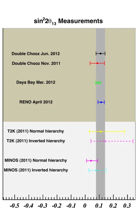
The first result from reactor experiment was released by Double Chooz in November 2011 [19] and shortly followed by Daya Bay [33] and RENO [31] in March 2012. In July 2012 Double Chooz released an updated analysis with twice the statistics and major improvements on many aspects of the
2.4 Measuring neutrino oscillation parameters 33 analyses [20]. The full and detailed description of the Double Chooz analysis is presented in Ch. 4.
Reactor ¯⌫e experiments are complementary to long baseline accelerator ex-periments in determining ✓13, since they are insensitive to the CP violating phase CP, and the dependence from the solar mass split is weak. Further-more, over short baselines of ⇠ 1 km the reactor ¯⌫e does not su↵er from matter e↵ects. Fig. 2.11 show a summary plot of the recent results from reactor and accelerator experiments.
2.4.4 Neutrino anomalies
So far neutrino oscillation is well established in terms of a three flavour framework. However, there are some experiments whose results are not ex-plained by this framework and might require the introduction of an extra sterile neutrino, i.e. a neutrino not participating in theSM interactions. The first evidence of more than three neutrino flavours came from the LSND experiment [27]. Using a ¯⌫µ from pion decay detected in a liquid scintilla-tor, LSND found > 3 evidence of ¯⌫µ ! ¯⌫e transition which would require a mass splitting of about 0.2 eV2, larger than the atmospheric one.
The LSND anomaly has been tested by MiniBooNE in both neutrino and an-tineutrino mode. The results obtained in the neutrino mode disfavour most of the parameter space defined by LSND but are not conclusive [28]. The results obtained in the antineutrino mode instead are consistent with LSND signal and consistent with a mass split of between 0.1 eV2 and 1 eV2 [29]. Further hints of the existence of sterile neutrinos came from measurements of neutrino fluxes from intense radioactive sources in the GALLEX [60] and SAGE [14] detectors. An unexpected reduction of the ⌫e flux consistent with ⌫e disappearance has been found at 2.7 . The interpretation in term of sterile neutrino oscillation indicates a value for the squared mass di↵er-ence of about 0.35 eV2.
Recent re-evaluation of the expected antineutrino flux from nuclear reactor indicate that the measured flux is about 3 % below the prediction with 3 significance [71]. Even if such a deficit could still be due to some unknown e↵ects in the reactor neutrino production or a non accurate knowledge of the fission product contribution to the antineutrino spectrum, it is consis-tent with ¯⌫e flux suppression due to sterile neutrino oscillation with mass split of about 2.4 eV2.
In summary, there are hints compatible with the existence of sterile neutrinos from several experiments, using di↵erent sources and detection technique, but none of them could claim a discovery. Many experiments have been pro-posed for for sterile neutrino search and an exhaustive list could be found in [12].
-0.5 -0.4 -0.3 -0.2 -0.1
0
0.1
0.2
0.3
-0.5 -0.4 -0.3 -0.2 -0.1
0
0.1
0.2
0.3
Double Chooz Nov. 2011
Daya Bay Mar. 2012
RENO April 2012
T2K (2011) Normal hierarchy T2K (2011) Inverted hierarchy
MINOS (2011) Normal hierarchy MINOS (2011) Inverted hierarchy
FIG. 16. Comparison of recent reactor- and accelerator-based
measurements of sin
2(2
13) from this analysis, the first
Dou-ble Chooz publication [4], Daya Bay [5], RENO [7], T2K [3],
and MINOS [2].
[28] Z. Djurcic et al., J. Phys. G36, 045002 (2009).
[29] W. Schreckenbach, G. Colvin, and F. von Feilitzsch,
Phys. Lett. 160B, 325 (1985).
[30] A. von Feilitzsch and K. Schreckenbach, Phys. Lett.
118B, 162 (1982).
[31] A. Hahn, K. Schreckenbach, W. Gelletly, F. von
Feil-itzsch, G. Colvin, and B. Krusche, Phys. Lett. B 218,
[36] G. Marleau et al., Report IGE-157 (1994).
[37] C. Jones, “Prediction of the Reactor Antineutrino Flux
for the Double Chooz Experiment”, Ph.D. thesis, MIT,
2012.
[38] C. Jones et al., arXiv:1109.5379v1 (2011).
[39] V. Kopeikin, L. Mikaelyan, and V. Sinev, Phys. At. Nucl.
67, 1892 (2004).
[40] Y. Declais et al., Phys. Lett. B338, 383 (1994).
[41] P. Vogel and J. F. Beacom, Phys. Rev. D 60, 053003
(1999).
[42] A. Pichlmaier et al., Phys. Lett. B 693, 221 (2010).
[43] J. Allison et al., IEEE Trans. Nucl. Sci. 53 No. 1 (2006)
270-278. S. Agostinelli et al., Nucl. Instrum. Meth. A506
(2003) 250-303.
[44] Apostolakis, J., Folger, G., Grichine, V., Howard, A.,
Ivanchenko, V., Kosov, M., Ribon, A., Uzhinsky, V.,
Wright, D. H., ”GEANT4 Physics Lists for HEP,”
Nuclear Science Symposium Conference Record, 2008,
IEEE, pp.833-836, 19-25 Oct. 2008.
[45] D. Motta and S. Schoenert, Nucl. Instrum. Meth. A539
(2005) 217.
[46] Tilley,
NucPhysA.745.155-362(2004),
Tilley,
NucPhysA.745.155-362(2004),
Y.
Prezado,
et
al,
Physics Letters B 618 (2005) 43.50, P. Papka, et al,
Phys. Rev. C 75, 045803 (2007).
[47]
http://www.chem.agilent.com/en-US/Products/instru-ments/molecularspectroscopy/fluorescence/systems/
caryeclipse/pages/default.aspx.
[48] C. Aberle, C. Buck, F.X. Hartmann, S. Sch¨
onert, S.
Wag-ner: JINST 6, P11006 (2011).
[49] Y. Abe et al., in preparation.
[50] P. Adamson et al., Phys. Rev. Lett. 106, 181801 (2011).
[51] H. Nunokawa et al., Phys. Rev. D72, 013009 (2005).
[52] G. Feldman and R. Cousins,
Phys.Rev.D57:3873-3889,1998.
[53] Proceedings of the XXXV International Conference on
Neutrino Physics and Astrophysics, June 3-19, 2012,
Ky-oto, Japan, to be published.
Figure 2.11: Comparison of recent reactor and accelerator-based measure-ments of sin2(2✓13) from Double Chooz [19] [20], Daya Bay [33], RENO [31], T2K [15], and MINOS [23]
2.5 The problem with the neutrino mass 35
2.5
The problem with the neutrino mass
As highlighted in Sec. 2.1,SM neutrinos are not allowed to acquire masses through the Higgs mechanism because they exist only in the left-handed chi-ral state (right-handed for anti-neutrinos). However, experimental evidences of neutrino oscillations imply the neutrino must be a massive particles. Further hints of a non-null neutrino mass also comes independently from neutrino oscillation. In particular, experiments looking for distortion in-duced by massive neutrinos on the -decay end point of tritium, 3H !3 He + e + ⌫e, limit ⌫e mass below 2 eV [41]. Similarly, the observation of the cosmic microwave background and the density fluctuations, and other cosmological measurements, put a combined upper limit on neutrino mass around 0.5 eV [76], which is six orders of magnitude smaller than the elec-tron mass. Is then necessary to extend theSM to include neutrino masses. The most natural extension of theSM add a right-handed neutrino singlet. In this case, neutrino masses are acquired through the Higgs mechanism, like all other fermions:
LD ' mD⌫L⌫R+ h.c. (2.20) the mass term is gauge invariant and conserves lepton number. The mD is the so called Dirac mass term and has the same form of the fermion masses in Eq. 2.3:
m⌫ = v p
2 ⌫ (2.21)
With this model the Yukawa coupling constant ⌫ ' m⌫/v needs to be of the order of 10 12, which is far too small compared to the other fermions ( e ⇠ 0.3 ⇥ 10 5) and it is commonly considered as unnatural.
Since neutrinos do not have electromagnetic charge, they could be described in term of a Majorana particles:
⌫c = C⌫T ⌘ ⌫ (2.22)
where ⌫c = C⌫T is the charge conjugate of the field ⌫c, and C is the charge conjugation. Considering a left-handed Majorana particle, ⌫ = ⌫L+ ⌫Lc, a Majorana mass term of the form:
LM ' mM⌫cL⌫L+ h.c. (2.23) could be considered. It should be noted that the Majorana mass term involves left-handed neutrino only and is not gauge invariant, m⌫c⌫ ! m⌫cei2↵⌫, violating lepton flavour number by two units.
The smallness of the neutrino mass term is no longer dependent on the unnatural Yukawa coupling constant, but nonetheless a mass term for a left-handed neutrino is not allowed by theSM because it implies an Higgs
LD+M = 1 2 ⌫ c L ⌫R mL mD mD mR ⌫L ⌫R + h.c. (2.25) The term mL is the left-handed neutrino Majorana mass, mR is the right-handed neutrino Majorana mass and mD is the Dirac mass. The mass matrix can be diagonalised in term of the mass eigenstate:
⌫L = cos ✓⌫1+ sin ✓⌫2 (2.26) ⌫Rc = sin ✓⌫1+ cos ✓⌫2 (2.27) with eigenstate m1,2: m1,2= 1 2 ✓ mL+ mR± q (mL mR)2+ m2D ◆ and tan 2✓ = 2mD mR mL (2.28) Since the left handed Majorana mass term requires an Higgs triplet, in the minimal SM extension, mL is usually set to zero. The right-handed Majorana neutrino is an electroweak singlet acquiring a mass independently from the Yukawa coupling.
In the limit where mL= 0 and mR mD: tan ✓' 2mD mR ' 0 ; m1' m2 D mR and m2' mR (2.29) with one light left-handed neutrino and one heavy right-handed neutrino:
⌫1 ' (⌫L ⌫Lc) (2.30)
⌫2 ' (⌫R+ ⌫Rc) (2.31) This is the so called see-saw mechanism, which involves two Majorana parti-cles: a very heavy right-handed neutrino and the observed light left-handed neutrino. The smallness of the observed neutrino mass could then be ex-plained in terms of a Dirac mass of the order of the electroweak energy scale, without the unnatural Yukawa coupling constant, and a much bigger Majo-rana mass term. The term mR is generally related to the grand unification
2.6 Summary and open questions 37 scale around the Planck scale at 1016 eV.
The Dirac or Majorana nature of the neutrino is not yet known. Experimen-tally it is possible to investigate this question through processes violating the lepton number like the neutrino-less double beta decay, which violated the lepton quantum number by two units. Many experiment are currently, or will soon, searching the neutrino-less double beta decay, CUORE [38], GERDA [22], EXO [49] and SUPER-NEMO [85], but not signal has been observed up to now.
2.6
Summary and open questions
Over the last twenty years many experimental e↵orts have provided clear confirmation that neutrinos are massive particle and that there is mixing between flavour and mass eigenstates. The status of the current knowledge is summarised in term of the mixing parameter and the mass splitting in Fig. 2.12 [41]. In Summary:
• The anomaly between the measured and the expected solar neutrino flux has been solved by SNO [30] and KamLAND [16]. The missing solar neutrino flux is interpreted within the neutrino oscillation sce-nario in term of ⌫e oscillation into a linear superposition of the three neutrino flavour.
The mixing angle is ✓12' 32 and m212 = (7.50± 0.20) ⇥ 10 5eV2. • The atmospheric neutrino oscillations has been characterised by SK [96] and long baseline accelerator experiment as K2K [32] and MINOS [24]. The observed disappearance of atmospheric ⌫µ has been inter-preted in term of oscillations into a linear superposition of, mainly, ⌫⌧ and ⌫µ. The most stringent limit on atmospheric neutrino oscillation parameters is provided by MINOS: sin22✓23 > 0.90 (90 % C.L.) and | m223| = (2.43 ± 0.13) ⇥ 10 3 eV2.
• The latest mixing angle ✓13is currently under measurement from accel-erator experiment, through ⌫µ! ⌫e appearance channel, and reactor experiments, through ¯⌫e disappearance. Measurements with sensitiv-ity > 3 has been recently published and further improvement are expected in the near future.
With the current characterisation of the PMNS matrix, new measurements will be possible in order to improve the current knowledge and to complete neutrino oscillation picture:
• The CP violation phase could be measured in long-baseline experi-ments, studying oscillation probability asymmetries between neutrino and antineutrino: P (⌫µ! ⌫e)6= P (¯⌫µ! ¯⌫e).
Figure 2.12: Summary of current knowledge on neutrino oscillation in m2 tan2✓. PDG 2011 update [41]. Does not contain yet 2012 results on ✓
2.6 Summary and open questions 39
In the next future, reactor experiments (Double CHOOZ and Daya Bay) and long
base-line neutrino experiments (T2K and Nova) will continue the search for ✓
13, increasing the
sensitivity of at least one order of magnitude with respect to the CHOOZ limit.
Figure 1.10: Normal and inverted neutrino mass orderings. The different colors show from
left to right the relative weights of the different flavor eigenstates (⌫
e, ⌫
µand ⌫
⌧) in a given
mass eigenstate.
If a non zero ✓
13will be discovered many new measurements in the neutrino physics will
be possible:
• the CP violating phase
can be measured in long-baseline experiments, studying
differences in the oscillation probability for neutrinos and antineutrinos, P (⌫
µ! ⌫
e)
6=
P (⌫
µ! ⌫
e)
• with long baselines it will be possible to use the oscillations in the matter to
dis-criminate the sign of
m
223. The sign of
m
223establishes the mass hierarchy of the
neutrinos. A positive
m
223
means that the neutrinos separated by the atmospheric
mass splitting are heavier than those separated by the solar mass splitting (normal
hierarchy) while a negative
m
223
indicates the opposite situation (inverted
hierar-chy). In the case of normal hierarchy,
m
223
> 0, the matter effects enhance ⌫
µ$ ⌫
eoscillations, suppressing ⌫
µ$ ⌫
ewhile in the case
m
223< 0 the opposite will happen;
23
Figure 2.13: The normal and inverted neutrino mass hierarchy. The di↵erent colours show the weights of the flavour mixing for a given mass eigenstate.
• The matter e↵ect2 could be used in long baseline experiment to mea-sure the sign of m2
23 and establish the neutrino mass hierarchy. As shown in Fig. 2.13, a positive (negative) m2
23 imply the neutrino separated by the atmospheric mass splitting is heavier (lighter) than the neutrinos separated by the solar mass splitting. In case of normal hierarchy, m2
23> 0, the matter e↵ect would enhance the ⌫µ$ ⌫e os-cillations while suppressing the ¯⌫µ$ ¯⌫e. In case of inverted hierarchy,
m223< 0, the opposite would happen.
• A combination of reactor ¯⌫edisappearance and both accelerator ⌫µ dis-appearance and ⌫eappearance would discriminate the sign of ✓23 ⇡/4. The degeneracy on the measurement of ✓23 at accelerator experiment will be broken by the reactor ✓13measurement which does not depend on ✓23. Such measurement would allow to discriminate the fraction of ⌫µ and ⌫⌧ contained by the mass state ⌫3.
Beyond neutrino oscillation, is then necessary to measure the absolute mass of the neutrinos, their Dirac or Majorana nature and to confirm or reject the existence of a fourth sterile neutrino.
![Figure 2.2: m 2 12 and ✓ 12 parameters from global analysis of solar and reactor experiments [91].](https://thumb-eu.123doks.com/thumbv2/123doknet/2318542.28469/26.892.246.574.226.544/figure-m-parameters-global-analysis-solar-reactor-experiments.webp)
![Figure 2.6: m 2 23 and ✓ 23 parameters from global analysis of atmospheric and accelerator experiments [91].](https://thumb-eu.123doks.com/thumbv2/123doknet/2318542.28469/29.892.314.637.206.533/figure-m-parameters-global-analysis-atmospheric-accelerator-experiments.webp)
![Figure 2.10: m 2 13 and ✓ 13 parameters from global analysis of reactor, at- at-mospheric and accelerator experiments [91].](https://thumb-eu.123doks.com/thumbv2/123doknet/2318542.28469/33.892.324.648.190.534/figure-parameters-global-analysis-reactor-mospheric-accelerator-experiments.webp)
![Figure 2.12: Summary of current knowledge on neutrino oscillation in m 2 tan 2 ✓. PDG 2011 update [41]](https://thumb-eu.123doks.com/thumbv2/123doknet/2318542.28469/39.892.229.728.183.970/figure-summary-current-knowledge-neutrino-oscillation-pdg-update.webp)