The comparison between two mortar spectral element methods for Darcy’s equations

(1)

HAL Id: tel-02901567

https://tel.archives-ouvertes.fr/tel-02901567

Submitted on 17 Jul 2020

HAL is a multi-disciplinary open access

archive for the deposit and dissemination of sci-entific research documents, whether they are pub-lished or not. The documents may come from teaching and research institutions in France or abroad, or from public or private research centers.

L’archive ouverte pluridisciplinaire HAL, est destinée au dépôt et à la diffusion de documents scientifiques de niveau recherche, publiés ou non, émanant des établissements d’enseignement et de recherche français ou étrangers, des laboratoires publics ou privés.

The comparison between two mortar spectral element

methods for Darcy’s equations

Kangzheng Xing

To cite this version:

Kangzheng Xing. The comparison between two mortar spectral element methods for Darcy’s equa-tions. Spectral Theory [math.SP]. Université Pierre et Marie Curie - Paris VI, 2015. English. �NNT : 2015PA066740�. �tel-02901567�

(2)

(3)

Dedicace

Cette thèse est dédiée aux membres de ma famille, sans lesquels je n’aurais jamais vu le jour.

(4)

(5)

Remerciements

Le thèse est un projet qui exige de l’endurance, de l’engagement et de la patience. A travers les quatre dernières années que je suis un doctorant à UPMC, je rencontrais des gens qui m’aidé avec la charge émotionnelle et scientifique qui vient avec un travail de ce genre. À la fin de ce travail, je tiens à exprimer ma gratitude et à adresser quelques mots à tous ceux qui, de près ou de loin, ont été présents et ont contribué à sa réalisation.

Je tiens tout d’abord à exprimer ma profonde reconnaissance envers Christine BERNARDI. Ces années de thèse sous sa direction furent pour moi un vrai enrichisse-ment. Je le remercie d’avoir accepté d’encadrer cette thèse. J’ai pu bénéficier de son intuition mathématique. Je voudrais le remercier pour tous ses encouragements constants, sa disponibilité et sa profonde gentillesse qui m’ont permis d’avancer sere-inement dans mon travail. Je n’oublierai jamais son soutien et sa disponibilité dans les moments de doute.

Juger un travail de thèse n’est pas une chose aisée. Pour cela, je suis extrêmement honorée que Madame Florence Hubert et Monsieur Mejdi Azaiez aient accepté de consacrer du temps à lire ce mémoire et à rédiger un rapport. Ils ont également contribué par leurs remarques et suggestions à améliorer la qualité de ce mémoire, et je les en remercie. Je leur suis également très reconnaissante d’avoir pris la peine de se déplacer pour assister à ma soutenance.

(6)

Dedicace

Je tiens à remercier très vivement M. Yvon Maday qui me fait l?honneur de présider mon jury de thèse. Je souhaiterais remercier le Professeur Faker Ben Bel-gacem qui a eu la gentillesse de me conseiller, pour le temps qu’il m’a accordé à plusieurs reprises au cours de cette thèse ainsi que pour l’intérêt qu’il a porté à mes travaux.

J’adresse une pensé particulière à Khashayar Dadras et Christian David pour son sourire, sa disponibilité, sa gentillesse et son amitié. Je le remercie également pour l’impression de ce manuscript malgré son état de santé. Je remercie Antoine Le Hyaric pour les nombreuses fois où il m’a aidée avec toutes sortes de problèmes (logiciels scientifiques ou autres) ainsi que pour son amitié et sa gentillesse à mon égard.

Je voudrais remercier mes collègues dans bureau 1516-316 qui m’ont accompagné pendant ces années de ma thèse à Jussieu, j’ai connu des nouvaux collègues dans bureau 1516-303 qui je remercie pour les nombreuses fois où il m’a aidé. Je voudrais remercier pour ces années passées au laboratoire Jacques-Louis Lions tous ses mem-bres pour la bonne humeur, l’atmosphère à la fois studieuse.

Je souhaiterais remercier mes rapporteurs pour le temps qu’ils ont accordé à la lecture de cette thèse et à l’élaboration de leur rapport.

Je remercie mes amis chinois de Paris pour l’ambiance amicale qu’ils ont créée, je pense à Ma Yue, Zhu Jiamin, Guo Hao et bien d’autres.

Je remercie particulièrement Yang Xingdi de m’avoir beaucoup aidé et accompa-gné. Merci à lui pour les moments agréables que nous avons passés ensemble à Paris. Merci pour son soutien et pour tout ce qu’elle a fait pour moi.

(7)

Chapter 1 Introduction

Motivation

In this thesis, we mainly talk about the problem of the flow of a viscous incom-pressible fluid moving in a rigid porous inhomogeneous medium. A good example of this problem is that water moves in the subsurface.

In the subsurface, rock is deposited in layers. Fluid flow within and between the rock layers is governed by the permeability of the rocks. However, to account for permeability, it must be measured in both the vertical and horizontal directions. For example, shale typically has permeabilities that are much lower vertically than hor-izontally (assuming flat lying shale beds). This means that it is difficult for fluid to flow up and down through a shale bed but much easier for it to flow from side to side. Ultimately, if the pressure difference between a hydraulically fractured zone and a fresh water aquifer is not great, the distance between the zones is relatively large, and there are rocks with low vertical permeabilities in between the deeper and the shallower zones, flow between the zones is unlikely to occur. The exception to this is where there is a separate flow pathway such as an open bore hole or a series of faults or joints that intersect both the fractured zone and the fresh water aquifer. Under either of these circumstances, the pressure difference and distance will be the

(12)

Chapter 1. Introduction

determining factors as to whether fluid can migrate from the lower to the upper zone. The principle that governs how fluid moves in the subsurface is called Darcy’s law. Darcy’s law is an equation that defines the ability of a fluid to flow through a porous media such as rock. The law was formulated by Henry Darcy based on the results of experiments [33] on the flow of water through beds of sand. It also forms the scientific basis of fluid permeability used in the earth sciences, particularly in hydrogeology. Although Darcy’s law (an expression of conservation of momentum) was determined experimentally by Darcy, it has since been derived from the Navier-Stokes equations via homogenization. It is analogous to Fourier’s law in the field of heat conduction, Ohm’s law in the field of electrical networks, or Fick’s law in diﬀusion theory.

One application of Darcy’s law is to water flow through an aquifer; Darcy’s law along with the equation of conservation of mass are equivalent to the groundwater flow equation, one of the basic relationships of hydrogeology. Darcy’s law is also used to describe oil, water, and gas flows through petroleum reservoirs.

Darcy’s law at constant elevation is a simple proportional relationship between the instantaneous discharge rate through a porous medium, the viscosity of the fluid and the pressure drop over a given distance. Darcy found that his data could be described by

U = kA µ

Pb Pa

L , (1.0.1)

where, U(units of volume per time, e.g., m3_/s_{) is equal to the product of the intrinsic}

permeability of the medium, k(m2_{), the cross-sectional area to flow, A (units of area,}

e.g., m2_{), (P}

b Pa)(Pascals) is the total pressure drop, and L, the length over which

the pressure drop.

The negative sign is needed because fluid flows from high pressure to low pressure. Note: the elevation head must be taken into account if the inlet and outlet are at diﬀerent elevations. If the change in pressure is negative (where Pa > Pb), then the

(13)

area and using more general notation leads

u = k

µ rP, (1.0.2)

where, u is the flux (discharge per unit area, with units of length per time, m/s) and rP is the pressure gradient vector (P a/m).

For very short time scales, a time derivative of flux may be added to Darcy’s law, which results in valid solutions at very small times (in heat transfer, this is called the modified form of Fourier’s law),

⌧@u

@t + u = k

µ rh, (1.0.3)

where ⌧ is a very small time constant which causes this equation to reduce to the normal form of Darcy’s law at "normal" times.

At last, in fact the water is the incompressible fluid, so the equation will also satisfy the incompressible condition:

r · (u) = 0.

A long this thesis we will focus on the following model : find a velocity u and pressure p solutions of : 8 > > > > > > < > > > > > > : ↵u + grad p = ↵f in ⌦, div u = 0 in ⌦, u · n = k on 1, p = p0 on 2 (1.0.4)

Spectral, spectral element and mortar element methods

Spectral methods are a class of techniques used in applied mathematics and scien-tific computing to numerically solve certain diﬀerential equations, often involving the

(14)

use of the Fast Fourier Transform. The idea is to write the solution of the differential equation as a sum of certain "basis functions" (for example, as a Fourier series which is a sum of sinusoids) and then to choose the coefficients in the sum in order to satisfy the differential equation as well as possible.

Spectral methods have been used extensively during the last decades for the nu-merical solution of partial diﬀerential equations (PDE) due to their bigger accuracy when compared to Finite Diﬀerences (FD) and Finite Elements (FE) methods. The rate of convergence of spectral approximations depends only on the smoothness of the solution, yielding the ability to achieve high precision with a small number of data. This fact is known in literature as "spectral accuracy".

Spectral element techniques are high order methods which allow for either obtain-ing very accurate results or reducobtain-ing the number of degrees of freedom for a fixed standard accuracy. As firstly explained by [51, 41], they rely on high degree piecewise polynomial approximation, and on the use of tensorized bases of polynomials.

For these reasons, the basic geometries for these methods are tensorized, i.e. they are square or cubes. We refer to [38, 43, 21] for a general presentation and analysis of the spectral methods in these geometries, and also to [36, 29, 55] for extensions to tri-angles or tetrahedra. The discrete spaces for spectral methods are simply polynomial spaces, and the discretization parameter is the maximal degree of these polynomials. The mortar element method, introduced in [24], is a domain decomposition tech-nique which allows for working on general partitions of the domain without con-formity restrictions. It is particularly important when combined with spectral-type discretizations, since handling complex geometries from very simple subdomains can be performed with this method in a very eﬃcient way. It can also be used to couple diﬀerent kinds of variational discretizations on the subdomains, such as finite ele-ments or spectral methods. So it leads to discrete problems which are most often non-conforming in the Hodge sense, which means that the discrete space is not

(15)

con-Chapter 1. Introduction

tained in the variational one. It was first analysed in the case of the 2D Laplace equation [24] which admits a natural variational formulation in the usual Sobolev space H1_(⌦) _{of functions with square-integrable first-order derivatives. We also refer}

to [9] for the first 3D results. It was extended [14] to the bilaplacian equation where the variational space is the standard space H2_(⌦)_{of functions with square-integrable}

first-order and second-order derivatives and also to the Stokes problem which is of saddle-point type; however, it still involves the usual Sobolev spaces. We also quote [13] for an application of the mortar technique to weighted Sobolev spaces, in order to handle discontinuous boundary conditions for the Navier-Stokes equations.

Objectives of the thesis

In this thesis, we mainly talk about the analysis of the mortar spectral element discretization of the problem (5.1.1 where ⌦ be a bounded, connected, open set in Rd_{, d = 2 or 3, with a Lipschitz continuous boundary @⌦, and let n denote the unit}

outward normal vector to ⌦ on @⌦, 1 and 2 be a partition of @⌦ without overlop. ↵

is constant or piecewise continuous coeﬃcients. The data are now the function f and the boundary conditions k and p0 . The unknowns are the velocity u and the pressure

(or hydraulic head, according to the model) p. we are interested in the case where this function is not globally continuous but only piecewise smooth and also such that the ratio of its maximal value to its minimal value is large. This models, for instance, the flow of a viscous incompressible fluid in a rigid porous inhomogeneous medium. A very interesting and unusual feature of Darcy’s equations is that they admit two equivalent variational formulations, whether the space of velocities is more regular than the space of pressures or not, see [6, 2, 19]. The drag coeﬃcient ↵ will be con-sidered as piecewise constant or piecewise smooth functions. The variational spaces can be choosen as (u; p) in H(div; ⌦) ⇥ L2_(⌦) _{or in L}2_(⌦)_{⇥ H}1_{(⌦). So two mortar}

discrete problems based on Galerkin numerical integration (GNI) will be constructed. Then we obtain the well-posedness and regularity properities of the problems. Next, it is necessary to prove a priori error estimates of spectral type: the order of convergence

(16)

only depends on the regularity of the solution, more precisely on its local regularity in each subdomain. For the implementation of the mortar technique, it mainly relies on an appropriate treatment of the matching conditions on the interfaces.

In this thesis, we will also develop a spectral method for fourth-order diﬀerential equa-tions in one dimension. A Legendre Petrov-Galerkin method for linear fourth-order diﬀerential equations and a Legendre Petrov-Galerkin and Chebyshev Collocation method for the nonlinear Kuramoto-Sivashinsky equation will be presented. Also we will prove the optimal rate of convergence in L2 _{norm of the method, and numerical}

experiments will be given which demonstrate the eﬃcient of proposed schemes.

Thesis outline

The thesis is composed by 2 parts. The first part is dedicated to the main subject of my work and concerns the numerical analysis of the martar method applied to the Darcy problem. During the first part of my thesis I worked on the analysis of a Legendre Petrov-Galekin method for linear fourth-order diﬀerential equations in one dimension and a Legendre Petrov-Galerkin and Chebyshev collocation method for the nonlinear Kuramoto-Sivashinsky equation have been developed. The second part contains the description of this contribution This invesgation will be given in the end of then mauscrit (see Appendix).

After a short introduction given in chapter one, we will consider in chapter 2 the Darcy’s equations with general boundary conditions and piecewise continuous coeﬃ-cients in a bounded domain. This problem can be formulated in two diﬀerent spaces. Then we prove the well-posedness of the equivalent variational problem of the Darcy’s equation. We also give the regularity properties.

In chapter 3 we present the discretization of the steady Darcy problem. We propose spectral discretizations of this problem based on the Galerkin with Numerical Inte-gration (G-NI) variants. The Numerical analysis of the discrete problem is performed. We also present the two-dimensional numerical experiments.

(17)

piecewise continuous coeﬃcients in a bounded domain. This problem can be formu-lated in spaces of square-integrable functions with square-integrable divergence. We propose a spectral element discretization of this problem which relies on the mortar domain decomposition technique. The Numerical analysis of the discrete problem is performed. We also present the two-dimensional numerical experiments. They turn out to be in good coherency with the theoretical results.

In chapter 5 we also consider Darcy’s equations with general boundary conditions and piecewise continuous coeﬃcients in a bounded domain. A spectral element discretiza-tion of this problem relies on the mortar domain decomposidiscretiza-tion technique is proposed. We present the numerical analysis and two-dimensional numerical experiments, which turn out to be in good coherency. This chapter ends with the comparison of the two spectral element methods will be presented in Chapter 6.

(18)

(19)

Chapter 2 Darcy’s Equations

2.1 Introduction

We first talk about the analysis of the mortar spectral element discretization of the problem introduced by Darcy [33] as follows

8 > > > > > > < > > > > > > : ↵u + grad p = ↵f in ⌦, div u = 0 in ⌦, u · n = k on 1, p = p0 on 2 (2.1.1)

where ⌦ is a bounded, connected, open set in Rd_{, d equals to 2 or 3, with a Lipschitz}

continuous boundary @⌦, and n denotes the unit outward normal vector to ⌦ on @⌦,

1 and 2, with a positive measure, being a partition of @⌦ without overlop. The

data are now the equation f and the boundary conditions k and p0 . The unknowns

are the velocity u and the pressure (or hydraulic head, according to the model) p. The coeﬃcients ↵ are constant or piecewise continuous. We are interested in the case where this function is not globally continuous but only piecewise smooth and also such

(20)

Chapter 2. Darcy’s equations

that the ratio of its maximal value to its minimal value is large. This models, for instance, the flow of a viscous incompressible fluid in a rigid porous inhomogeneous medium.

2.2 Sobolev spaces

In this section, we recall the main notions and results, concerning the classical Sobolev spaces, which will be used in later sections, also some properties. Although they are stated without proof, these results are complete, rigorous and fairly general. We define D(⌦) to be the linear space of infinitely diﬀerentiable functions, with compact support on ⌦. Then we set

D( ¯⌦) =_{{ |}⌦; 2 D(Rd)}

or equivalently, if O denotes any open subset of RN _{such that ¯⌦ ⇢ O,}

Now, let D0

(⌦) denote the dual space of D(⌦), often called the space of distribu-tions on ⌦. We denote by < ·, · > the duality pairing between D0

(⌦) and D(⌦) and we remark that when f is locally integrable function, then f can be identified with a distribution by

< f, >= Z

⌦

f (x) (x)dx, _{8 2 D(⌦)}

In other words, < ·, · > is an extension of the scalar product of L2_(⌦)_.

For v = (v1, v2, ..., vN), we define the divergence operator by:

div v =

N

X

i=1

(21)

Note the identity:

div (gradv) = 4v.

So far, we have been mainly interested in subspaces of H1_(⌦)N_{; but subsequently,}

it will be worthwhile to use functions with less regularity. Bearing this in mind, we introduce the following spaces:

H(div ; ⌦) =_{{v 2 L}2(⌦)N; divv 2 L2(⌦)_}, which is clearly a Hilbert space for the norm:

||v||H(div ;⌦) = (||v||20,⌦+||div v||20,⌦)1/2. (2.2.1)

Next we are coming to the trace theorems. The trace on the boundary of a function v 2 Hs_(⌦) _{is ,in a sense to make precise, the value of v restricted to . If}

we denote by C0_{( ¯}_⌦) _{the space of continuous functions on ¯⌦, the precise result reads}

as follows, see ([40], Chapter I):

Theorem 2.1 Let ⌦ be a bounded open set of RN _{with Lipschitz-continuous boundary}

and let s > 1/2.

1. There exists a unique linear continuous map 0 : Hs(⌦) ! Hs 1/2( ) such that 0v = v| for each v 2 Hs(⌦).

2. There exists a linear continuous map R0 : Hs 1/2( )! Hs(⌦) such that 0R0' =

' for each ' 2 Hs 1/2_{( ).}

The next theorem concerns the normal component of boundary values of functions of H(div ; ⌦).

Theorem 2.2 The mapping n : v ! v · n| defined on D(¯⌦)N can be extended by

continuity to a linear and continuous mapping, still denoted by n, from H(div ; ⌦)

(22)

By extension, nv is called the normal component of v on and is denoted simply

by v · n.

From the above two theorem, we derive the following Green’s formula:

(v, grad ) + (div v, ) =< v · n, > , 8v 2 H(div ; ⌦), 8 2 H1(⌦). (2.2.2) As a consequence, we can now extend Green’s formula for the Laplace operator to a wider range of functions.

Corollary 2.1 Let u 2 H1_(⌦) _{and 4u 2 L}2_(⌦)_{. Then @u/@n 2 H} 1/2_{( )} _and

(grad u, grad v) = (4u, v)+ < @u/@n, v > , 8v 2 H1(⌦). (2.2.3)

Two useful applications of Green’s formula will also be given here.

Lemma 2.1 Let ⌦ be a bounded open subset of RN _{with a Lipschitz-contunuous}

boundary .

1. For u and v in H1_(⌦) _{and for 1  i  N, we have}

Z ⌦ u(@v/@xi)dx = Z ⌦ (@u/@xi)vdx + Z 0u 0vnids (2.2.4) 2. If in addition u 2 H2_(⌦) _{we have} N X i=1 Z ⌦ @u @xi @v @xi dx = N X i=1 Z ⌦ @2_u @x2 i + N X i=1 Z (@u @xi v)nids (2.2.5)

Adopting the usual notations

4u = N X i=1 @2_u @x2 i

(23)

(2.2.5) becomes:

(gradu, gradv) = (4u, v) + Z

(@u/@n) 0vds. (2.2.6)

When ⌃ is an open (non-empty) Lipschitz continuous subset of the boundary , we introduce the space

H_⌃1(⌦) :=_{{v 2 H}1(⌦)_| ⌃v = 0}.

An important result, which will find widespread application in the sequel, is the so-called Poincaré inequality, see ([25], Chapter 1, Lemma 2.6):

Theorem 2.3 Assume that ⌦ is a bounded connected open set of RN_{. Then there}

exists a constant C⌦(⌃) > 0 such that

Z ⌦ v2₍_{x)dx  C} ⌦(⌃) Z ⌦|rv(x)| 2_d_x _(2.2.7) for each v 2 H1 ⌃(⌦).

We next recall Sobolev embedding theorem ([3], Chapter 4).

Theorem 2.4 Assume that ⌦ is a (bounded or unbounded) open set of Rd _{with a}

Lipschitz continuous boundary, and that 1  p < 1. Then the following continuous embedding hold:

1. If 0  sp < d, then Ws,p_(⌦)_{⇢ L}p⇤

(⌦) for p⇤ _{= dp/(d} _sp);

2. If sp = d, then Ws,p_(⌦)_{⇢ L}q_(⌦) _{for any q such that p  q < 1;}

3. If sp > d, then Ws,p_(⌦)_{⇢ C}0_{( ¯}_⌦)_.

2.3 Variational formulations

A very interesting feature of Darcy’s equations is that they admit two equivalent variational formulations, whether the space of velocities is more regular than the space

(24)

of pressures or not, see [6, 2, 19]. The drag coeﬃcient ↵ will be considered as piecewise constants or piecewise smooth functions. The variational spaces can be choosen as (u; p)in H(div ; ⌦) ⇥ L2_(⌦) _{or in L}2_(⌦)_{⇥ H}1_(⌦)_{. So two variational formulations will}

be constructed.

Throughout the thesis, we make the following assumptions on the function ↵: there exists a finite number of domains ⌦l, 1 l  L, such that :

• they form a partition of ⌦ without overlapping:

¯ ⌦ = L X l=1 ¯ ⌦l, ⌦l\ ⌦l0 =;, 1  l 6= l 0  L, (2.3.1)

•the restriction of ↵ to each ¯⌦l, 1 l  L, is bounded and positive, i,e. there exists

constants ↵max

l and ↵minl such that

↵max_l = sup x2 ¯⌦l ↵(x) < +1, ↵min_l = inf x2 ¯⌦l ↵(x) > 0. (2.3.2) We set ↵max = max 1lL↵ max l , ↵min = min 1lL↵ min l . (2.3.3)

2.3.1 Velocity in H(div , ⌦)

In this subsection, for each domain O in Rd_{with a Lipschitz-continuous boundary,}

we use the full scale of Sobolev spaces Hs₍_{O) and H}s

0(O), s 0, their trace spaces

on @O and their dual spaces. We denote by C1_{( ¯}_{O) the space of restrictions to O of}

indefinitely diﬀerentiable functions of Rd _{and by D(O) its subspace of functions with}

a compact support in O.

Let be any part of @⌦ with positive measure. We also recall that H12

00( )is defined as

the space of functions in H1

(25)

We have the following formula

8q 2 H12 00( ), < (v · n), q(x) >= Z ⌦ (div v) ¯q(x)dx + Z ⌦v · (grad ¯q)(x)dx

where ¯q is any lifting in H1_(⌦) _{of the extension by zero of q to @⌦. So the normal}

trace on of a function v in H(div , ⌦) makes sense in the dual space H12

00( )

0

of H12

00( ). In fact, the integral in the left-hand side of the above equality represents a

duality pairing. We next define

H0(div , ⌦) ={v 2 H(div , ⌦); v · n = 0 on @⌦} (2.3.4)

Then D(⌦)d _{is dense in H}

0(div , ⌦), and both H0(div , ⌦) and H(div , ⌦) are Hilbert

spaces for the scalar product associated with the norm defined in (2.2.1). We now introduce the variational spaces

X(⌦) = H(div , ⌦),

X0(⌦) ={v 2 X(⌦); v · n = 0 on 1}.

(2.3.5)

Both of them are equipped with the norm

||v||X(⌦) =||v||H(div ,⌦) = (||v||2_L2_(⌦)d+||div v||2_L2_(⌦)) 1

2. (2.3.6)

The variational problem we consider reads: Find (u, p) in X(⌦) ⇥ L2_(⌦) _{such that}

u · n = k on 1 and that

8v 2 X0(⌦), a↵(u, v) + b(v, p) = L(v),

(26)

where the bilinear forms and linear form are defined by

a↵(u, v) = L X l=1 ↵l Z ⌦l u(x) · v(x)dx, b(v, q) = Z ⌦ (divv)(x) · q(x)dx. L(v) = L X l=1 ↵l Z ⌦l f(x) · v(x)dx Z 2 p0(s) (v · n)(s)ds

We make the following assumption on the data

f 2 X0(⌦) 0 , k _{2 (H}12 00( 1)) 0 , p0 2 H 1 2 00( 2), (2.3.8)

2.3.2 Velocity in L

2

_(⌦)

The variational problem that we consider now reads : Find (u, p) in L2_(⌦)d_⇥

H1_(⌦) _{such that p = p} 0 on 2 and that 8v 2 L2_(⌦)d_, _a ↵(u, v) + b(v, p) = L(v), 8q 2 H1 2(⌦), b(u, q) = R 1k(⌧ ) q(⌧ )d⌧, (2.3.9)

where the bilinear forms and linear form are defined by

a↵(u, v) = L X l=1 ↵l Z ⌦l u(x) · v(x)dx, (2.3.10) b(v, q) = Z ⌦v(x) · (grad q)(x)dx. (2.3.11) and L(v) = Z ⌦ ↵f(x) · v(x)dx (2.3.12) H1₂(⌦) ={q 2 H1_{(⌦), q = 0 on} 2}. (2.3.13)

(27)

2.4 Well-posedness of the problem

2.4.1 Case of velocity in H(div , ⌦)

Proposition 2.1 Assume that the partition of @⌦ into 1 and 2 is suﬃciently

smooth for D(⌦ [ 2) to be dense in X0(⌦). If the data (f, k, p0) satisfy

assump-tion (2.3.8), any smooth enough pair of funcassump-tions (u, p) in X(⌦)⇥L2_(⌦) _{is a solution}

of problem (2.3.7) if and only if it is a solution of problem (2.1.1).

Proof: We refer to [15]. If Y (⌦) = D(¯⌦)(¯⌦) \ X0(⌦), then Y (⌦) is dense in X0(⌦).

When multiplying the first line in (2.1.1) by a function v in Y (⌦), integrating by parts, we obtain that the first equation of (2.3.7) is satisfied for all v in Y (⌦), hence for all vin X0(⌦)by density. Conversely, letting v run through D(⌦[ 2)\ X0(⌦)gives the

first line of (2.1.1) in the distribution sense and letting v run through Y (⌦) leads to the fourth line. Due to the density of D(⌦) in L2_{(⌦), the second line in (2.1.1), when}

taken in the distribution sense, is fully equivalent to the second equation in (2.3.7). To prove the well-posedness of problem (2.3.7), we first construct a lifting of the boundary conditions. Before that we introduce the ↵-dependent norms

||v||↵,X(⌦)= ( L X l=1 ↵l(||v||2L2_(⌦ l)d +||div v|| 2 L2_(⌦_l₎)) 1 2 (2.4.1) ||q||↵⇤,L2_(⌦) = ( L X l=1 1 ↵l||q||L 2_(⌦_l₎) 1 2 (2.4.2)

Lemma 2.2 There exists a divergence-free function ub in X(⌦) which satisfies

(28)

Chapter 2. Darcy’s equations and ||ub||↵,X(⌦)  C p↵max||k|| (H 1 2 00( 1))0 . (2.4.4)

where C is dependent with ↵.

Proof: We now denote by I(⌦) the space

I(⌦) ={µ 2 H1_{(⌦); µ = 0 on}

2},

and we consider the problem : Find in I(⌦) such that ,

8µ 2 I(⌦), R⌦(grad ) · (gradµ)(x)dx =

R

1(k µ)(x)d⌧ (2.4.5)

This problem has a unique solution. Moreover the function ub =grad is

divergence-free on ⌦ and satisfies ub· n = k on 1, and

||ub||↵,X(⌦)  C p↵max||k|| (H 1 2 00( 1))0 . (2.4.6)

To go further, we set: u0 =u ub, and consider the following problem: Find (u0, p)

in X0(⌦)⇥ L2(⌦) such that

8v 2 X0(⌦), a↵(u0,v) + b(v, p) = a↵(ub,v) + L(v),

8q 2 L2_{(⌦), b(u}

0, q) = 0.

(2.4.7)

Then we can see that the kernel

V (⌦) ={v 2 X0(⌦);8 q 2 L2(⌦), b(v, q) = 0} (2.4.8)

coincides with the space of functions in X0(⌦) which are divergence-free on ⌦. So it

(29)

Lemma 2.3 The following ellipticity property holds

8v 2 V (⌦), a↵(v, v) = ||v||2↵,X(⌦). (2.4.9) Proof: 8 v 2 V (⌦), a↵(v, v) = L P l=1 ↵l R ⌦lv · vdx = ||v|| 2 ↵,X(⌦).

Lemma 2.4 There exists a constant > 0 such that the following inf-sup condition holds 8q 2 L2_(⌦), _sup v2X0(⌦) b(v, q) ||v||↵,X(⌦) r ↵min ↵max||q||↵ ⇤_,L2_(⌦). (2.4.10)

Proof: We first define the space

W ={x|x 2 H1_(⌦), _{x = 0 on}

2},

then for all q 2 L2_(⌦), _{their exists Y 2 W , such that}

8 > > > < > > > : Y = q, in ⌦ gradY · n = 0, on 1 Y = 0 on 2 (2.4.11)

Letting v = grad Y , then v 2 X0(⌦) and div v = q in ⌦. Obviously,

b(v, q) = Z

⌦

div v q dx = ||q||2_L2_(⌦).

Thanks to Green’s formula and Poincaré-Friedrichs inequality

||grad Y ||2L2_(⌦) = Z ⌦ q Y dx  ||q||L2_(⌦)||Y ||_H1_(⌦)  c||q||_L2_(⌦)||grad Y ||_L2_(⌦). It follows with ||v||L2_(⌦) =||grad Y ||_L2_(⌦)  c||q||_L2_(⌦)

(30)

Chapter 2. Darcy’s equations So ||v||↵,X(⌦) = ( L X l=1 ↵l(||v||2L2_(⌦ l)d+||div v|| 2 L2_(⌦_l₎)) 1 2  Cp↵_max||q||_L2_(⌦)

Then we obtain the result

8q 2 L2_(⌦), _sup v2X0(⌦) b(v, q) ||v||↵,X(⌦) c r ↵min ↵max||q||↵ ⇤_,L2_(⌦).

It follows from Lemma 2.3 and Lemma 2.4 that problem (2.4.7) has a unique solution (u0, p) in X0(⌦)⇥ L2(⌦) and that this solution satisfies

||u0||↵,X(⌦)+ c r ↵min ↵max||p||↵ ⇤_,L2_(⌦)  C 1 p ↵min (_||ub||↵,X(⌦)+||f||L2_(⌦)+||p₀|| H12 00( 2) ) (2.4.12) We now obtain the main result of this section.

Theorem 2.5 For any data satisfying (2.3.8), problem (2.3.7) has a unique solution (u, p) in X(⌦) ⇥ L2_(⌦). _{Moreover this solution satisfies}

||u||↵,X(⌦)+ c r ↵min ↵max||p||L 2_(⌦)  c 1 p_↵ min (p↵max||k|| (H12 00( 1))0 +_||f||L2_(⌦)+||p₀|| H12 00( 2) ). (2.4.13)

2.4.2 Case of velocity in L

2

_(⌦)

Proposition 2.2 Assume that the partition of @⌦ into 1 and 2 is suﬃciently

smooth for D(⌦ [ 1) to be dense in H12(⌦). Any smooth enough pair of functions

(u, p) is a solution of problem (2.3.9) if and only if it is a solution of problem (2.1.1) in the distribution sense.

Proof: Due to the density of D(⌦)d _{in L}2_(⌦)d_{, the first line in (2.1.1), when taken}

in the distribution sense, is fully equivalent to the first equation in (2.3.9). On the other hand, when multiplying the second line in (2.1.1) by a function q in D(⌦ [ 1),

(31)

integrating by parts and using the third line, we obtain that the second equation of (2.3.9) is satisfied for all q in C1_(⌦)_{\ H}1

2(⌦), hence for all q in H

1

2(⌦) by density

according to [15]. Conversely, letting q run through D(⌦ [ 1) gives the second line

of (2.1.1) in the distribution sense and letting q run through C1_(⌦)_{\ H}1

2(⌦) leads

to the third line.

We now introduce the ↵-dependent norms

||v||↵ = ( L X l=1 ↵l||v||2L2_(⌦)d) 1 2, ||q||_↵ ⇤ = ( L X l=1 1 ↵l|q| 2 H1_(⌦ l)) 1 2 (2.4.14)

To prove the well-posedness of problem (2.3.9), we first cite the following Property ([48], Chap. I, § 11).

Property 2.1 For all p0 2 H

1 2

00( 2), the extension ˜p0 by zero from 2 to @⌦, such

that ˜p0| 2 = p0 belongs to H 1

2(@⌦) and satisfies || ˜p₀||

H12(@⌦)  C ||p0||_H12 00( 2).

Then we construct a lifting of the boundary conditions of ˜p0. We give the following

lemma.

Lemma 2.5 There exists a linear continuous map R0 : Hs 1/2( ) ! Hs(⌦) such

that R0p˜0 = ¯P, and inf 0( ¯P )= ˜p0|| ¯ P_||H1_(⌦)=|| ˜p₀|| H12(@⌦)  C||p0||_H12 00( 2) (2.4.15)

To go further, we set: P1 = p P¯, and consider the following problem: Find

(u, P1) in L2(⌦)d⇥ H1₂(⌦) such that

8v 2 L2_{(⌦), a}

↵(u, v) + b(v, P1) = b(v, ¯P ) +L(v),

8q 2 H1

2(⌦), b(u, q) =< k, q > 1 .

(32)

Indeed, the form a↵(·, ·) and b(·, ·) satisfy the continuity properties and we have the

ellipticity property

8 v 2 L2(⌦)d, a↵(v, v) = ||v||2↵. (2.4.17)

We also have the inf-sup condition on the form b(·, ·) as follows:

Lemma 2.6 8 q 2 H12(⌦), sup v2L2_(⌦)d b(v, q) ||v||↵ ||q|| ↵_⇤ (2.4.18) Proof: 8 q 2 H1 2(⌦), letting v = ↵ 1_{rq, then v 2 L}2_(⌦)d_{. b(v, q) =} R ⌦v · rq = ||q||2 ↵⇤ So b(v,q)_||v||_↵ ||q|| 2 ↵⇤ ||q||↵⇤ ||q||↵⇤

It follows from (2.4.17) and (2.4.18) that problem (2.4.16) has a unique solution (u, P1) in L2(⌦)d⇥ H1₂(⌦) and that this solution satisfies

||u||↵+||P1||↵⇤  C(||f||↵+|| ¯P||↵⇤) (2.4.19)

We are now state the main result of this section.

Theorem 2.6 For any data (f, k, p0)in L2(⌦)d⇥H

1

2( ₁)⇥H 1 2

00( 2), problem (2.3.9)

has a unique solution (u, p) in L2_(⌦)d_{⇥ H}1_(⌦). _{Moreover this solution satisfies}

||u||↵+||p||↵⇤  C(||f||↵+||p0|| H 1 2 00( 2) +p↵max||k|| (H 1 2 00( 1))0 ). (2.4.20)

Proof: We establish successively the existence and uniqueness of the solution. 1) It follows from the Lax-Milgram lemma, combined with Bramble-Hilbert inequality, that there exists a unique µ in H1

2(⌦) such that

8' 2 H12(⌦),

Z

⌦

(33)

Thus, the function ub =grad µ satisfies

||ub||↵  cp↵max||k|| (H 1 2 00( 1))0 . (2.4.22)

On the other hand, it follows from the standard results on saddle-point problems ([40], Chap,I, Cor.4.1) that the problems

Find (u0, P1) in L2(⌦)d⇥ H1₂(⌦) such that

8v 2 L2_{(⌦), a}

↵(u0,v) + b(v, P1) = b(v, ¯P ) a↵(ub,v) + L(v),

8q 2 H1

2(⌦), b(u0, q) = 0.

(2.4.23)

has a unique solution (u0, P1)which morever satisfies

||u0||↵+||P1||↵⇤  C(||ub||↵+||f||↵+|| ¯P||↵⇤) (2.4.24)

Then, the pair (u, p) with u = u0 +ub, p = P1 + ¯P, is a solution of problem

(??)-(2.3.9), and estimate (2.4.20) follows from (2.4.22) and (2.4.24). The pair(u = u0+ub, p = P1+ ¯P )is a solution of problem (??)-(2.3.9), and estimate (2.4.20) is a

consequence of (2.4.15) and (2.4.19). On the other hand, let (u1, p1) and (u2, p2) be

two solutions of problem (2.3.9). Then the diﬀerence (u1 u2, p1 p2) is a solution

of problem (2.4.16) with data ub,f, P1 equal to zero, also p0 equal to zero. Thus, it

follows from (2.4.20) that it is zero. So the solution of problem (2.3.9) is unique.

2.5 Regularity properties

Let O be a subdomain of ⌦ such that ↵ is a constant in a neighbourhood of ¯O in ⌦. We first set

(34)

Then we introduce a space

W0 ={u 2 H(curl, div ; O)|u · n 2 L2(@O)}.

Due to ([5], Remark 2.16) and [30], when O is a general Lipschitz domain, the space W0 is imbedded in H

1

2(O). When the domain O is convex, due to ([5], Theorem

2.17), then the space W0 is continuously imbedded in H1(O), in fact, u · n has even

higher regularity, u · n 2 H1

2(@O). In the subdomain O, taking the curl of the first

equation in (2.1.1), yields

curl (↵u) = curl (↵f) in O.

This leads to the following local regularity result.

Proposition 2.3 Let O be a subdomain of ⌦ such that ↵ is a constant in a neigh-bourhood of ¯O in ⌦. Then the mapping: (f, k, p0) 7! (u, p), where (u, p) is the

so-lution of problem (2.1.1), is continuous from Hs_(⌦)d _{⇥ H}s 1₂_(⌦) _{⇥ H}s+1₂_(⌦) _into

Hs₍_O)d_{⇥ H}s+1₍_{O), (i) for 0  s } 1

2 in the general case, (ii) for 0  s  1 when ¯O

is convex.

It follows from [31] that these results still hold with O replaced by O \ ⌦l

i) in dimension d = 2, when the ⌦l are polygons and ¯O does not contain any

vertex of the ⌦l,

ii) in dimension d = 3, when the ⌦l are polyhedras and ¯O neither contains a vertex

of the ⌦l nor intersects an edge of the ⌦l.

However when ¯O either contains a vertex of the ⌦l or intersects an edge of the ⌦l and

(35)

properties can be proved only in dimension d = 2 and thus we only consider this case in what follows.

We first consider the local regularity properties. We introduce here also a space

W ={u 2 H(curl, div ; ⌦)|u · n 2 L2_(@⌦)_}.

We know from [30] when ⌦ is a polygon, a function u in W can be written as

u = ur+gradS, (2.5.1)

where ur belongs to H1(⌦)2 and S is a linear combination of the singularities of the

Laplace equation provided with Neumann boundary conditions. We recall that each singularity in the neighbourhood of a corner of the polygon with aperture ! has the form

r⇡!('(✓) + (logr)p (✓)),

where r is the distance to the corner, ✓ the corresponding angular variable, p is equal to 0 except when ⇡

! is an integer where it is equal to 1. More generally, any such

function u which has the further property

div u 2 Hs(⌦), curl u 2 Hs(⌦)3, (2.5.2) admits the expansion (2.5.1) with ur in Hs+1(⌦)2 for all s, 0 < s < 2⇡_! 1.

Taking the curl of the fisrt equation in (2.1.1), which yields

curl (↵u) = curl (↵f) in ⌦.

So when ⌦ is a polygon, u admits the expansion (2.5.1), and if curl f belongs to Hs_(⌦)2_{, 0 < s <} 2⇡

! 1, where ! denotes the largest angle of ⌦, the regular part ur

in this expansion belongs to Hs+1_(⌦).

(36)

(2.1.1), we consider the following mixed boundary conditions problem: 8 > > > < > > > :

div (_↵1 grad p) = div f in ⌦,

1

↵@n p =f · n on ,

p = p0 on 2

(2.5.3)

We know from [34] that there exists a real number s0, 0 < s0 < 1₂,only depending

on the geometry of ⌦, ↵min and ↵max, such that when div f 2 Hs 1(⌦) and p0 2

Hs+

1 2

⌃ ( 2), the solution p of the equation (2.5.3) belongs to Hs+1(⌦) for all s  s0,

where Hs+12

⌃ ( 2) stands for the space of functions such that their restrictions to any

edge e contained in ¯2 belongs to Hs+

1

2(e). Morever, when ⌦ is a polygon, according

to ([42],Chapter 5) and [34], p will belong to Hs+1_{(⌦), s}_{ min{s}

0,2⇡_! 1}.

We then consider the local regularity properties when ¯O contains either vertex of the ⌦l or intersects an edge of the ⌦l. we are now at the last conclusion of this section.

Suppose f|⌦l, k, p0 belongs to H

sl_(⌦

l)2⇥ Hsl

1

2(⌦_l)⇥ Hsl+12(⌦_l) for any real positive

number sl: i) When ¯⌦l contains no corner of ⌦, the regularity of (u, p) on ⌦l only

depends on the data f, and (u, p) belongs to Hsl_(⌦

l)2⇥ Hsl+1(⌦l).

ii) When ¯⌦l contains a corner of ⌦ with !, we derive from (2.5.1) that u|⌦l =

ur+grad S, p|⌦l = pr+ S. So the first equation of (5.1.1) can be rewritten as

1 ↵grad p 0 =f urwherep 0 = pr+ (1 + ↵) S. (2.5.4)

Taking the curl of the first equation of (5.1.1) and taking div of the equation (2.5.4), we can get that (ur, pr)belongs to Hs(⌦l)2⇥ Hs+1(⌦l) for s  sl and s < 2⇡_!.

(37)

Chapter 3 Spectral Discretization of Darcy’s

Equations

3.1 Orthogonal polynomials

We firstly work on the interval ⇤ = [ 1, 1], since all results on ⌦ are deduced from their analogues on ⇤ thanks to tensorization arguments. Over ⇤, all the approxima-tion properties rely on a proper choice of an orthogonal basis of L2_{(⇤) :}_{the Legendre}

polynomials.

The family of Legendre polynomials is a family (Lk)k 0 of polynomials in one

variable, which are orthogonal to each other in L2_{(⇤). For any integer k} _{0, the}

polynomail Lk has degree k. If Lk(x) is normalized so that Lk(1) = 1, then for any

k: Lk(x) = 1 2k [k/2] X (l=0) ( 1)l ✓ k l ◆✓ 2k 2l k ◆ xk 2l, (3.1.1) where [k/2] denotes the integral part of k/2.

(38)

Chapter 3. Spectral Discretization of Steady Darcy’s Equations

also that the polynomial Lk is even if k is even and odd if k is odd.

The norm of each Lk is given by the formula

Z 1 1

L2_k(x)dx = 1

k + 1₂. (3.1.2) We recall from ([1], Chapter 22) some very important properties of these polynomials, firstly the diﬀerential equation

((1 x2_)L0

k)

0

+ k(k + 1)Lk= 0, k 0, (3.1.3)

secondly the integral equation

(2k + 1)Lk = L

0

k+1 L

0

k 1, k 1, (3.1.4)

thirdly the induction formula, which allows for computing them:

Lk+1(x) = 2k + 1 k + 1 xLk(x) k k + 1Lk 1(x), (3.1.5) where L0(x) = 1 and L1(x) = x.

We consider now discrete Legendre series. Since explicit formulas for the quadra-ture nodes are not known, such points have to be computed numerically as zeros of approximate polynomials. The quadrature weights can be expressed in closed form in terms of the nodes, as indicated in the following formulas: ([44], Chapter 2)

• Legendre- Gauss (LG) : forj = 1, . . . , N

xj are zeros of LN +1; (3.1.6) !j = 2 (1 x2 j)[L 0 N +1(xj)]2 . (3.1.7)

(39)

• Legendre -Gauss-Lobatto (LGL) : forj = 0, . . . , N

xj are zeros of (1 x2)L 0 N; (3.1.8) !j = 2 N (N + 1) 1 [LN(xj)]2 . (3.1.9)

3.2 Quadrature Formula

As we know that, the most natural quadrature formula in the polynomial context is the Gauss Lobatto formula associated with the Lebesgue measure, since it allows for easily handling boundary conditions and leads to diagonal mass matrices. We firstly describe it, next we study the corresponding interpolation operators.

The Gauss Lobatto formula

Let us set x0 = 1 and xN = 1. There exists a unique set of N 1 nodes xj, 1 

j  N 1and a unique set of N + 1 weights ⇢j, 0 j  N, such that the following

exactness property holds

8 2 P2N 1(⇤), Z 1 1 (x)dx = N X j=0 (xj)⇢j. (3.2.1)

The zeros xj, 1  j  N 1, are the zeros of L0N and the weights ⇢j are positive,

given by ⇢j = 2 N (N + 1)L2 N(xj) , 0_{ j  N.} (3.2.2) We conclude with a further useful property of the quadrature formula.

Lemma 3.1 There exists a constant c such that

8 N 2 PN(⇤), || N||2L2_(⇤)  N X j=0 2 N(xj)⇢j  3|| N||2L2_(⇤). (3.2.3)

(40)

Proof: We write the expansion of any polynomial N in L2(⇤) :

N =

N

X

n=0

↵nLn. (3.2.4)

We deduce from the exactness property (3.2.1) that

|| N||2L2_(⇤)= N X n=0 ↵2_n_||Ln||2L2_(⇤), N X j=0 2 N(xj)⇢j = N 1_X n=0 ↵2_n||Ln||2L2_(⇤)+ ↵2_N N X j=0 L2_N(xj)⇢j,

so that it suﬃces to prove the results with N = LN. Noting that the degree of the

polynomial L2

N + N 2(1 x2)L

0₂

N is less than 2N 1 (this comes by computing the

coeﬃcient of x2N_{), we derive that}

Z 1 1 (L2_N(x) + N 2(1 x2)L0_N2(x))dx = N X j=0 (L2_N(xj) + N 2(1 x2j)L 0₂ N(xj))⇢j, (3.2.5)

or equivalently, since the xj are the zeros of (1 x2)L

0 N, N X j=0 L2 N(xj)⇢j = Z 1 1 L2 N(x)dx + N 2 Z 1 1 L02 N(x)(1 x2)dx. (3.2.6)

The second integral is easily computed, leading to

N X j=0 L2_N(xj)⇢j = (2 + 1 N)||LN|| 2 L2_(⇤). (3.2.7)

(41)

3.3 Polynomial approximation

3.3.1 Polynomial approximation on the interval

Let now N be a fixed positive integer 2. In what follow, c stands for a positive constant independent of N. We introduce the orthogonal projection operator ⇡N from

L2_(⇤) _{onto P}

N(⇤). Then the projection operator can be expressed in the following

way: 8 2 L2(⇤), ⇡N = N X n=0 n_L n, (3.3.1) where n= 1 ||Ln||2_L2_(⇤) Z 1 1 (x)Ln(x)dx. (3.3.2)

Lemma 3.2 For any real numbers s 0, the following estimate holds for any in Hs_(⇤)_:

|| ⇡N ||L2_(⇤)  cN s|| ||_Hs_(⇤). (3.3.3)

For the proof of this lemma, we propose ([23], Proposition 1). We now consider the orthogonal projection operator ⇡1,0

N from H01(⇤)onto P0N(⇤),

for the scalar product associated with the norm | · |H1_(⇤). Its properties are derived

from the formula (⇡1,0

N )

0

= ⇡N 1 0 for the bounded in H1(⇤), plus a duality argument

for the bounded in L2_(⇤)_.

Proposition 3.1 ([23], Proposition 2) For any real number s 1, the following estimate holds for any in Hs_(⇤)_{\ H}1

0(⇤):

| ⇡_N1,0 _|H1_(⇤)+ N|| ⇡1,0

N ||L2_(⇤)  cN1 s|| ||_Hs_(⇤). (3.3.4)

(42)

Chapter 3. Spectral Discretization of Steady Darcy’s Equations 0 defined by 0(x) = (x) ( 1) 1 x 2 (1) 1 + x 2 , (3.3.5) and since it belongs to H1

0(⇤), we define the polynomial ⇡N1 by

(⇡_N1 )(x) = (⇡_N1,0 0)(x) + ( 1)

1 x

2 + (1) 1 + x

2 . (3.3.6) This operator does not correspond to an orthogonal projection, but it preserves the values in ±1 and its properties are easily derived from the formula ⇡1

N = 0

⇡_N1,0 0.

Proposition 3.2 ([23], Proposition 3) For any real number s 1, the following estimate holds for any in Hs_(⇤)_{\ H}1

0(⇤):

| ⇡_N1 |H1_(⇤)+ N|| ⇡_N1 ||_L2_(⇤) cN1 s|| ||_Hs_(⇤). (3.3.7)

3.3.2 Polynomial approximation on the square or cube

For each n 0, let Pn(⌦) be the space of polynomials worth degree  n with

respect to each variable, and P0

nbe its subspace made of all polynomials which vanish

on the boundary @⌦.

As previously, we fix an integer N 2. The best fit of a given function is realized via projection operators onto PN(⌦) or P0N(⌦), and analyzing their properties relies

on tensorization arguments. For instance, if ⇧N denotes the orthogonal projection

operator from L2_(⌦)_{onto P}

N(⌦), it coincides with ⇡N(x) ⇡ (y)

N in dimension d = 2, with

⇡_N(x) ⇡(y)_N ⇡(z)_N in dimension d = 3, where the exponent after an operator denotes the direction in which it is applied. So the approximation properties of the operator ⇧N

are derived from the triangular inequality, in dimension d = 2 for instance:

(43)

Proposition 3.3 ([23], Proposition 4) For any real number s 0, the following estimate holds for any v in Hs_{(⌦) :}

||v ⇧Nv||L2_(⌦)  cN s||v||_Hs_(⌦). (3.3.9)

Let now ⇧1,0

N stand for the orthogonal projection operator from H01(⌦)onto P0N(⌦).

Using a further duality argument, we derive the next proposition.

Proposition 3.4 ([23], Proposition 5) For any real number s 1, the following estimate holds for any v in Hs_(⌦)_{\ H}1

0(⌦) :

|v ⇧1,0_N v|H1_(⌦)+ N||v ⇧_N1,0v||_L2_(⌦)  cN1 s||v||_Hs_(⌦). (3.3.10)

Finally, the approximation properties of the orthogonal projection operator ⇧1 N

from H1_(⌦) _{onto P}

N(⌦) are derived from the same triangular inequality .

Proposition 3.5 ([23], Proposition 6) For any real number s 1, the following estimate holds for any v in Hs_{(⌦) :}

|v ⇧1_Nv_|H1_(⌦)+ N||v ⇧_N1 v||_L2_(⌦)  cN1 s||v||_Hs_(⌦). (3.3.11)

3.4 Polynomial interpolation

In this section, we will introduce the interpolation operator on Gauss-Lobatto points.

(44)

3.4.1 Polynomial interpolation on the interval

Our aim is to derive the appxoximation properties of the Lagrange interpolation operator iN at the nodes xj, 0 j  N, with values in PN(⇤), which means that

(iN )(xj) = (xj), 0 j  N. (3.4.1)

Lemma 3.3 ([23], Lemma 3) There exists a positive constant c such that, for any function in H1

0(⇤),

||iN ||L2_(⇤) c(|| ||_L2_(⇤)+ N 1| |_H1_(⇤)). (3.4.2)

Applying the above inequality to the function ⇡1

N obviously gives an estimate

for the interpolation error of functions which belongs to H1_{(⇤). However, we have}

rather state a slightly more general result which allows for interpolating less smooth functions.

Proposition 3.6 ([23], Proposition 7) For any real number s > 1

2, the following

estimate holds for any in Hs_(⇤):

|| iN ||L2_(⇤)  cN s|| ||_Hs_(⇤). (3.4.3)

Proposition 3.7 ([21], Theorem 13.4) For any real number r and s satisfying s > max{1

2, r} and 0  r  1, there exists a postive constant c depending only on s such

that, for any function in Hs_(⇤)_{, the following estimate holds:}

(45)

3.4.2 Polynomial interpolation on the square or cube

By tensorization, we associate with the nodes xj the grid

⌅N = 8 < : {(xi, xj), 0 i, j  N} in dimension d=2, {(xi, xj, xk), 0  i, j, k  N} in dimensiond=3, (3.4.5)

and also the discrete product: for all continuous functions u and v on ¯⌦,

((u, v))N = 8 > > < > > : N P i=0 N P j=0 u(xi, xj)v(xi, xj)⇢i⇢j in dimensiond=2, N P i=0 N P j=0 N P k=0 u(xi, xj, xk)v(xi, xj, xK)⇢i⇢j⇢k in dimension d=3, (3.4.6)

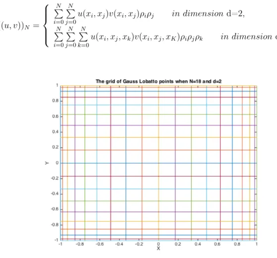
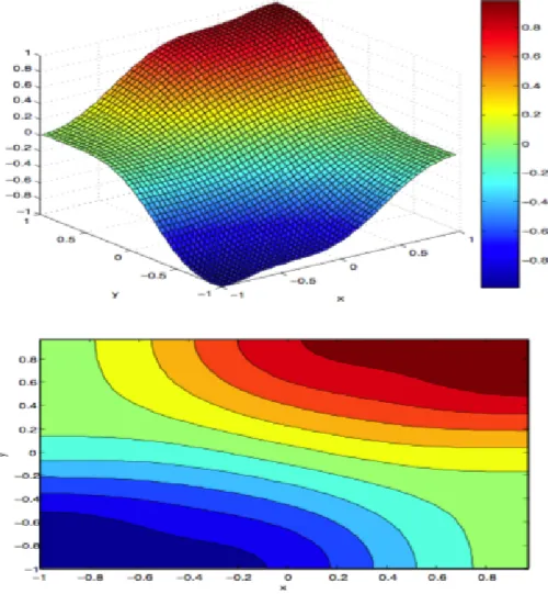
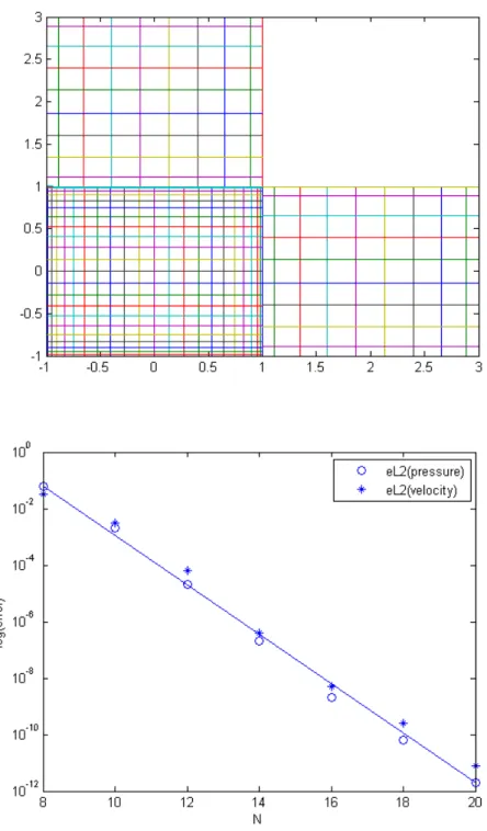
Figure 3-1: The Grid of Gauss Lobatto points when N=18 and d=2

We denote by IN the Lagrange interpolation operator on the grid ⌅N, with values

in PN(⌦). The operator coincides with i(x)_N i(y)_N in dimension d = 2, and with

i(x)_N i(y)_N i(z)_N in dimension d = 3. So, proving its approximation properties is now obvious.

(46)

Proposition 3.8 For any real number s > d

2, the following estimate holds for any v

in Hs_{(⌦) :}

||v INv||L2_(⌦)  cN s||v||_Hs_(⌦). (3.4.7)

For any real number r and s satisfying s > max{d

2, r} and 0  r  1, there exists a

postive constant c depending only on s such that, for any function in Hs_(⌦)_{, the}

following estimate holds:

|v INv|Hr_(⌦)  cNr s||v||_Hs_(⌦). (3.4.8)

3.5 Spectral discretization of the Darcy’s problem

According to the variational forms in Chapter 2, we here discuss the discrete problems.

3.5.1 First discretization

According to the variational formulation, we introduce the discrete spaces as fol-lows:

DN =PN(⌦)d, (3.5.1)

also we introduce another space:

D0

N ={uN 2 DN, uN · n = 0 on 1}. (3.5.2)

For the space of pressure, there are diﬀerent choices. Usually we consider the spurious modes on the pressure, namely the set

(47)

which is analyzed in [8] and [25]. The space of pressure MN will be taken as the

orthogonal space of Zn in PN.

But here we choose another pressure space as MN =PN 2(⌦)which has not been

discussed yet in the literature as far as the author’s knowledge. Assuming that the functions f, k, p0 has continuous restrictions to ¯⌦ and ¯1, ¯2 respectively. Then

the discrete problem built from the variational formulation reads: Find (uN, pN) in

DN ⇥ MN such that uN · n = IN1k on 1, (3.5.4) and 8vN 2 D0N, aN↵(uN,vN) + bN(vN, pN) =LN(vN), 8qN 2 MN, bN(uN, qN) = 0. (3.5.5)

where the bilinear forms aN

↵(·, ·) and bN(·, ·) are defined by

aN

↵(uN,vN) = ↵((uN,vN))N,

bN(vN, qN) = ((div vN, qN))N,

LN(vN) = ((↵ f, vN))N ((p0,vN · n))N2.

(3.5.6)

Next we introduce the ↵ dependent norms

||vN||↵ = (↵(||vN||2+||div vN||2)) 1 2, ||qN||↵⇤ = (↵ 1||qN||2) 1 2. (3.5.7)

Lemma 3.4 There exists a divergence-free function ub

N in DN which satisfies

ub

N · n = IN1k on 1, (3.5.8)

and

||ubN||↵  C p↵max||IN1k|| (H

1 2 00( 1))0

(48)

where C is dependent with ↵.

To go further, we set: u0

N = u ubN, and consider the following problem: Find

(u0

N, p) in D0N ⇥ MN such that

8vN 2 D0N, aN↵(u0N,v) + b(v, p) = aN↵(ubN,v) + LN(vN),

8q 2 MN, bN(u0N, q) = 0.

(3.5.10)

Then we can see that the kernel

VN ={vN 2 D0N;8 qN 2 MN, bN(vN, qN) = 0} (3.5.11)

coincides with the space of functions in D0

N which are divergence-free on ⌦. So it is

easy to have the following Lemma about aN ↵(·, ·):

Lemma 3.5 There exists a constant c independent of the discretization, such that the following ellipticity property holds

8vN 2 VN, aN↵(vN,vN) c||vN||2↵. (3.5.12)

Next, we come to the inf-sup condition.

Lemma 3.6 There exists a constant > 0 such that the following inf-sup condition holds 8qN 2 MN, sup vN2D0N bN(vN, qN) ||vN||↵ ||qN||↵ ⇤. (3.5.13)

Proof: The proof is given only in the case d = 2, since the corresponding proof in the case d = 3 is completely similar. Any function qN in MN has the expansion

qN(x, y) = N 2_X m=0 N 2_X n=0 ↵mnLm(x)Ln(y). (3.5.14)

(49)

We can derive that

||qN||2L2_(⌦)= N 2_X m=0 N 2_X n=0 ↵_mn2 1 (m + 1 2)(n + 1 2) (3.5.15)

The idea is now to choose vN = (v1N, v2N), with

v1N(x, y) = N 2_X m=0 m X n=0 ↵mn Lm+1(x) Lm 1(x) 2m + 1 Ln(y) (3.5.16) and v2N(x, y) = N 2_X m=0 N 2_X n=m+1 ↵mnLm(x) Lm+1(y) Lm 1(y) 2m + 1 . (3.5.17) In fact, the polynomial vN belongs to D0N, and which satisfies div vN = qN. Next,

we note that @v1N(x, y) @x = N 2 X m=0 m X n=0 ↵mnLm(x)Ln(y) (3.5.18)

which allows for bounding ||@v1N(x,y)

@x ||L2(⌦)by comparing with (3.5.15). Using a similar

argument for @v2N(x,y)

@y , we derive that

||@v1N(x, y)

@x ||L2(⌦)+||

@v2N(x, y)

@y ||L2(⌦)  c||qN||L2(⌦), (3.5.19) and also, thanks to the Poincaré-Friedrichs inequality applied with respect either to x or y,

||v1N(x, y)||L2_(⌦)+||v2_N(x, y)||_L2_(⌦)  c||q_N||_L2_(⌦), (3.5.20)

then the inf-sup condition is obviously.

It follows from Lemma 3.5.12 and Lemma 3.6 that problem (3.5.10) has a unique solution (u0

N, p) in D0N ⇥ MN and that this solution satisfies

||u0||↵+||p||↵⇤  C(||u_b||_↵+||I_Nf||_L2_(⌦)d+||I_N2p₀||

H12 00( 2)

) (3.5.21) We now state the main result of this section.

(50)

Theorem 3.1 For any data (f, k, p0)such that each f, and k, p0 are continuous on ¯⌦k

and on 1, 2, problem (3.5.4) (3.5.5) has a unique solution (uN, pN) in DN ⇥ MN.

Moreover this solution satisfies

||uN||↵+||pN||↵⇤  c(||I_N1k|| (H12 )0 00 ( 1) +_||INf||L2_(⌦)d+||I_N2p₀|| H12 00( 2) ). (3.5.22)

Proof: The pair(u = u0

N+ubN, p)is a solution of problem (3.5.4)-(3.5.5), and estimate

(3.5.22) is a consequence of (3.5.21) and (3.5.62). On the other hand, let (u1, p1)and

(u2, p2)be two solutions of problem (3.5.4)-(3.5.5). Then the diﬀerence (u1 u2, p1

p2)is a solution of problem (3.5.10) with data ub,f, p0 equal to zero. Thus, it follows

from (3.5.22) that it is zero. So the solution of problem (3.5.4)-(3.5.5) is unique.

• Error estimate : here we introduce a new norm as follows:

||uN||↵,L2_(⌦) = (↵||u_N||2) 1 2.

We prove an error estimates, first for the velocity, second for the pressure. Let u be the solution of equation (2.1.1), uN the solution of equation (3.5.4)-(3.5.5) and !!!N

any function in the kernal VN(⌦). Multiply the first line of (2.1.1) by !!!N gives

↵ Z ⌦ u0 · !!!Ndx + b(!!!N, p) = ↵ Z ⌦f · !!! Ndx ↵ Z ⌦ ub· !!!Ndx. (3.5.23)

Using the definition of VN(⌦) thus implies, for any qN in MN(⌦),

↵ Z ⌦ u0· !!!Ndx + b(!!!N, p qN) = ↵ Z ⌦f · !!! Ndx ↵ Z ⌦ ub· !!!Ndx. (3.5.24)

(51)

In (3.5.24), letting !!!N =u0N vN and subtracting the first line of (3.5.10) leads to

||u0 N vN||2↵,L2_⌦ ↵ Z ⌦ (u0 vN)· (u0N vN)dx + ↵ Z ⌦ vN · (u0N vN)dx ↵((vN,u0N vN))kN + b(uN0 vN, p qN) + ↵((f, u0N vN))kN ↵ Z ⌦f · (u 0 N vN)dx + ↵ Z ⌦ ub_{· (u}0 N vN)dx ↵((ub N,u0N vN))kN + Z 2 p0· [(u0N vN)· n]ds ((p0, (u0N vN)· n))_N2. (3.5.25)

Using a triangle inequality yields

||u uN||↵,L2_(⌦)  ||u₀ v_N||_↵,L2_(⌦)+||u0_N v_N||_↵,L2_(⌦)+||u_b ub_N||_↵,L2_(⌦)

 C{ inf_v N2VN||u 0 vN||↵,L2_(⌦)+ sup !!!N2DN {↵ R ⌦vN · !!!Ndx ↵((vN, !!!N)) k N ||!!!N||↵,L2_(⌦) +↵((f,!!!N)) k N ↵ R ⌦f · !!!Ndx ||!!!N||↵,L2_(⌦) + ↵R_⌦ub · !!!Ndx ↵((ubN, !!!N))kN ||!!!N||↵,L2_(⌦) + R 2p0· (!!!N · n)ds ((p0, (!!!N · n)) 2 N ||!!!N||↵,L2_(⌦) + b(!!!N, p qN) ||!!!N||↵,L2_(⌦) +||ub u b N||↵,L2_(⌦)}. (3.5.26) All the items above can be found in ([25], Chapter V), we will not prove here and we will give the first theorem about the velocity as follows.

Theorem 3.2 Assume that the solution (u, p) of the problem (2.1.1) in Hm_(⌦)d_⇥

Hm(⌦) for m d/2; the function f belongs to Hm_(⌦)d _{for m} _d/2_{; the function}

k on 1 in Hs( 1) for s > d 1₂ , and p0 on 2 in Ht(⌦) for t > d 1₂ , we have the

following estimate:

||u uN||↵,L2_(⌦)  c(N m(||u||_Hm_(⌦)d+||p||_Hm_(⌦))

+N r_||f||Hr_(⌦)d+ N s||k||_Hs₍ ₁₎+ N t||p₀||_Ht₍ ₂₎).

(3.5.27)

Due to the inf sup condition, for any qN in MN(⌦), we derive that

D||pN qN||↵⇤  sup vN2D0N(⌦) R ⌦(pN qN)(div vN)dx ||vN||↵ . (3.5.28)

(52)

In order to evaluate R_⌦(pN qN)(div vN)dx, we first use the discrete problem

(3.5.5): Z ⌦ (pN qN)(div vN)dx = ↵((f, vN))kN ((p0,vN · n))N2 ↵((uN,vN))kN + Z ⌦ qN(div vN)dx. (3.5.29)

Next, we apply equation (2.1.1) to the function vN, integrate by parts and add it to

the previous line, which yields Z ⌦ (pN qN)(div vN)dx = ↵((f, vN))kN ↵ Z ⌦f · v Ndx +↵ Z ⌦u · v Ndx ↵((u, vN))kN + Z 2 p0· (v · n) ds ((p0,vN · n))N2+ Z ⌦ (qN p) divvNdx (3.5.30)

Now, it is easy to derive the next theorem.

Theorem 3.3 Assume that the solution (u, p) of the problem 2.1.1 in Hm_(⌦)d _⇥

Hm_(⌦) _{for m} _d/2_{; the function f belongs to H}m_(⌦)d _{for m} _d/2_{; the function}

k on 1 in Hs( 1) for s > d 1₂ , and p0 on 2 in Ht(⌦) for t > d 1₂ , we have the

following estimate:

||u uN||↵,L2_(⌦)+||p p_N||_↵⇤  c(N m(||u||_Hm_(⌦)d +||p||_Hm_(⌦))

+N r_||f||Hr_(⌦)d+ N s||k||_Hs₍ ₁₎+ N t||p₀||_Ht₍ ₂₎).

(3.5.31)

3.5.2 Second discretization

• Well-posedeness of the solution : According to the variational formulation, we introduce the discrete spaces as follows:

(53)

also we introduce another space:

M1

N ={qN 2 MN, qN = 0 on 2}. (3.5.33)

Assuming that the functions f, k, p0 has continuous restrictions to all ¯⌦k, 1  k 

K and ¯1, ¯2 respectively. Then the discrete problem built from the variational

formulation reads: Find (uN, pN) in XN ⇥ MN such that

pN = p0 on 2, (3.5.34)

and

8vN 2 XN, aN↵(uN,vN) + bN(vN, pN) =LN(vN),

8qN 2 M1N, bN(uN, qN) = ((k, qN))N1.

(3.5.35)

where the bilinear forms aN

↵(·, ·) and bN(·, ·) are defined by

aN

↵(uN,vN) = ↵((uN,vN))N,

bN(vN, qN) = ((vN,grad qN))N,

LN(vN) = ((↵ f, vN))N.

(3.5.36)

We introduce here related norm and semi-norm as follows:

||uN||↵ = (↵||uN||2)

1

2, ||q_N||_↵_⇤ = (↵ 1|q_N|2) 1 2.

We construct a lifting of the boundary condition of p0, we give the following lemma

according to the reference ([25], Th. III.3.1) or ([7], Lemma 4.1).

Lemma 3.7 If p0 is continuous on 2, then there exists a function pbN in MN and a

constant c independent of N, such that

pb_N =_I 2

(54)

Chapter 3. Spectral Discretization of Steady Darcy’s Equations and ||pb N||↵⇤  c r 1 ↵min ||I 2 N p0||_H1 2( 2). (3.5.38) To go further, we set p0

N = pN pbN, and consider the following problem: Find

(uN, p0N) in XN ⇥ M1N such that

8vN 2 XN, aN↵(uN,vN) + bN(vN, p0N) = LN(vN) bN(vN, pbN),

8qN 2 M1N, bN(uN, qN) = ((k, qN))N1.

(3.5.39)

Lemma 3.8 The form aN

↵(·, ·) satisfies the following continuity and ellipticity

prop-erties

8uN 2 XN,8vN 2 XN, aN↵(uN,vN) c||uN||↵||vN||↵, (3.5.40)

8uN 2 XN, aN↵(uN,uN) ||uN||2↵. (3.5.41)

Proof: We use the Cauchy-Schwarz inequality to (3.4.6), we can derive

((u, v))N  ((u, u))

1 2 N((v, v)) 1 2 N. (3.5.42)

For all uN in XN, because ↵k is piecewise constant, we have

aN_↵(uN,uN) = ↵ N X i=0 N X j=0 u2 N(xi, xj)⇢i⇢j, (3.5.43)

then we can easily derive:

8uN 2 XN,||uN||2↵  aN↵(uN,uN) c||uN||2↵. (3.5.44)

(55)

Lemma 3.9 The bilinear form bN(·, ·) satisfies the inf-sup condition

8qN 2 M1N, sup

vN2XN

bN(vN, qN)

||vN||↵

C ||qN||↵⇤. (3.5.45)

Proof: We note that for any qN in M1N, we can define the function vN by

vN = ↵ 1gradqN, (3.5.46)

It is obvious that vN 2 XN. Then we have the above inf-sup condition. From

(3.5.40-3.5.41) and the inf-sup condition (3.5.45), the saddle-point problem (3.5.39) has a unique solution (uN, p0N) which satisfies

||uN||↵+||p0N||↵⇤  C (||pb_N||_↵⇤+||I_N1k||

H 12( 1)+||INf||L

2_(⌦)d) (3.5.47)

Now we are in the position of the main result of this section:

Theorem 3.4 For any data (f, k, p0)such that each f, and k, p0 are continuous on ¯⌦k

and on 1, 2 respectively, problem (3.5.34) (3.5.35) has a unique solution (uN, pN)

in XN ⇥ MN. Moreover, there exists a constant c independent of N such that this

solution satisfies ||uN||↵+||pN||↵⇤  C (||I_N2p₀|| H12( 2)+||I 1 N k||_H 12( 1)+||INf||L 2_(⌦)d) (3.5.48)

Proof: We establish successively the existence and uniqueness of the solution. 1) It follows from the Lax-milgram lemma, combined with Bramble-Hilbert inequality, that there exists a unique 'N in XN such that