HAL Id: tel-00770663
https://tel.archives-ouvertes.fr/tel-00770663
Submitted on 7 Jan 2013
HAL is a multi-disciplinary open access
archive for the deposit and dissemination of
sci-entific research documents, whether they are
pub-lished or not. The documents may come from
L’archive ouverte pluridisciplinaire HAL, est
destinée au dépôt et à la diffusion de documents
scientifiques de niveau recherche, publiés ou non,
émanant des établissements d’enseignement et de
Formation of stars and star clusters in colliding galaxies
Pierre-Emmanuel Belles
To cite this version:
Pierre-Emmanuel Belles. Formation of stars and star clusters in colliding galaxies. Other.
Uni-versité Paris Sud - Paris XI; University of Hertfordshire (Hatfield (GB)), 2012. English. �NNT :
2012PA112312�. �tel-00770663�
UNIVERSITE PARIS-SUD et UNIVERSITY OF HERTFORDSHIRE
ÉCOLE DOCTORALE : ED127
Laboratoire Astrophysique, Interactions, Multi-échelles (AIM)
(Service d'Astrophysique du CEA-Saclay)
DISCIPLINE : Astrophysique
THÈSE DE DOCTORAT
soutenue le 28/11/2012par
Pierre-Emmanuel BELLES
Formation d'étoiles et d'amas stellaires
dans les collisions de galaxies
~
Formation of stars and star clusters
in colliding galaxies
Directeur de thèse : Pierre-Alain DUC Docteur (Laboratoire AIM)
Co-directeur de thèse : Elias BRINKS Professeur (University of Hertfordshire)
Composition du jury :
Président du jury : Guillaume PINEAU-DES-FORETS Professeur (Université Paris-Sud XI)
Rapporteurs : Martin HARDCASTLE Docteur (University of Hertfordshire) Pascale JABLONKA Docteur (École Polyt. Fédérale de Lausanne)
A mon grand p`ere Aim´e,
qui a des ´etoiles plein les yeux quand je lui parle d’astronomie; Et `a ma grand m`ere Marie,
English abstract
Mergers are known to be essential in the formation of large scale structures and to have a significant role in the history of galaxy formation and evolution. Besides a morphological trans-formation, mergers induce important bursts of star formation. These starburst are characterised by high Star Formation Efficiencies (SFEs) and Specific Star Formation Rates, i.e., high Star Formation Rates (SFR) per unit of gas mass and high SFR per unit of stellar mass, respectively, compared to spiral galaxies. At all redshifts, starburst galaxies are outliers of the sequence of star-forming galaxies defined by spiral galaxies.
We have investigated the origin of the starburst-mode of star formation, in three local interact-ing systems: Arp 245, Arp 105 and NGC 7252. We combined high-resolution JVLA observations of the 21-cm line, tracing the H i diffuse gas, with UV GALEX observations, tracing the young star-forming regions. We probe the local physical conditions of the Inter-Stellar Medium (ISM) for independent star-forming regions and explore the atomic-to-dense gas transformation in dif-ferent environments. The SFR/H i ratio is found to be much higher in central regions, compared to outer regions, showing a higher dense gas fraction (or lower H i gas fraction) in these regions. In the outer regions of the systems, i.e., the tidal tails, where the gas phase is mostly atomic, we find SFR/H i ratios higher than in standard H i-dominated environments, i.e., outer discs of spiral galaxies and dwarf galaxies. Thus, our analysis reveals that the outer regions of mergers are characterised by high SFEs, compared to the standard mode of star formation.
The observation of high dense gas fractions in interacting systems is consistent with the predictions of numerical simulations; it results from the increase of the gas turbulence during a merger. The merger is likely to affect the star-forming properties of the system at all spatial scales, from large scales, with a globally enhanced turbulence, to small scales, with possible modifications of the initial mass function. From a high-resolution numerical simulation of the major merger of two spiral galaxies, we analyse the effects of the galaxy interaction on the star forming properties of the ISM at the scale of star clusters. The increase of the gas turbulence is likely able to explain the formation of Super Star Clusters in the system.
Our investigation of the SFR–H i relation in galaxy mergers will be complemented by high-resolution H i data for additional systems, and pushed to yet smaller spatial scales.
R´
esum´
e en Fran¸cais
Les fusions sont un ´ev`enement essentiel dans la formation des grandes structures de l’Univers; elles jouent un rˆole important dans l’histoire de formation et l’´evolution des galaxies. Outre une transformation morphologique, les fusions induisent d’importants sursauts de formation d’´etoiles. Ces sursauts sont caract´eris´es par des Efficacit´es de Formation Stellaire (EFS) et des Taux de Formation Stellaire Sp´ecifiques (TFSS), i.e., respectivement, des Taux de Formation Stellaire (TFS) par unit´e de masse gazeuse et des TFS par unit´e de masse stellaire, plus ´elev´es que ceux des galaxies spirales. A toutes les ´epoques cosmiques, les galaxies `a sursaut de formation d’´etoiles sont des syst`emes particuliers, en dehors de la s´equence d´efinie par les galaxies spirales.
Nous explorons l’origine du mode de formation stellaire par sursaut, `a travers trois syst`emes in interaction: Arp 245, Arp 105 et NGC 7252. Nous avons combin´e des observations JVLA haute r´esolution de la raie `a 21-cm, tra¸cant le gaz H i diffus, avec des observations GALEX dans l’UV, tra¸cant les jeunes r´egions de formation d’´etoiles. Nous sommes ainsi en mesure de sonder les conditions physiques locales du Milieu InterStellaire (MIS) pour des r´egions de formation d’´etoiles ind´ependantes, et d’´etudier la transformation du gaz atomique en gaz dense dans diff´erents environnements. Le rapport SFR/H i apparaˆıt bien plus ´elev´e dans les r´egions centrales que dans les r´egions externes, indiquant une fraction de gaz dense plus ´elev´ee (ou une fraction de gaz H i moins ´elev´ee) dans les r´egions centrales. Dans les r´egions externes des syst`emes, i.e., les queues de mar´ees, o`u le gaz est dans une phase principalement atomique, nous observons des rapports SFR/H i plus ´elev´es que dans les environnements standards domin´es par le H i, i.e., les r´egions externes des disques de spirales et les galaxies naines. Ainsi, notre analyse r´ev`ele que les r´egions externes de fusions sont caract´eris´ees par des EFS ´elev´ees, par comparaison au mode de formation stellaire standard.
Observer des fractions de gaz dense ´elev´ees dans les syst`emes en interaction est en accord avec les pr´edictions des simulations num´eriques; ceci r´esulte d’une augmentation de la turbulence du gaz durant une fusion. La fusion affecte les propri´et´es de formation stellaire du syst`eme probablement `a toutes les ´echelles, depuis les grandes ´echelles, avec une turbulence augmentant globalement, jusqu’aux petites ´echelles, avec des modifications possibles de la fonction de masse initiale. A partir d’une simulation num´erique haute r´esolution d’une fusion majeure entre deux galaxies spirales, nous analysons les effets de l’interaction des galaxies sur les propri´et´es du MIS `
a l’´echelle des amas stellaires. L’accroissement de la turbulence du gaz explique probablement la formation de Super Amas Stellaire dans le syst`eme.
Notre ´etude de la relation SFR–H i dans les fusions de galaxies sera compl´et´ee par des donn´ees H i haute r´esolution pour d’autres syst`emes, et pouss´ee vers des ´echelles spatiales encore plus petites.
Acknowledgements
First of all, I’d like to thank my supervisors: Elias & Pierre-Alain. If I have the first part in this story, they have undoubtedly the second parts. They have always been present when I needed them, they advised me, they supported me and, of course, they taught me what being a scientist is. Because knowledge is freedom of mind, I’ll be grateful to them for the rest of my life. Their kindness and human qualities make me proud of having studying / working with them. Besides, I’d like to thank Fr´ed´eric Bournaud, who kept a mindful eye on my work and with whom I had very useful discussions, as well as Martin Hardcastle and Pascale Jablonka, the “rapporteurs” of this dissertation, the members of the jury (made of the two rapporteurs, Carole Mundell, Frank Bigiel, Guillaume Pineau-des-Forˆets and my supervisors), Pierre-Olivier Lagage and Michel Talvard, the heads of the department, Marc Sauvage, the head of the scien-tific team. I also thank Pascale Chavegrand and Christine Toutain not only for their help with administrative paperwork, but also for their kindness.
Then, there would be no thesis if Florent Renaud, Roger Leiton, St´ephanie Juneau, Katarina Kraljic, Kevin DeGiorgio, Mark Sargent, Joana Gomez, Harriet Parson, Luke Hindson were not here day-after-day. Because having support from young postdocs, other PhD students or office-mates is essential, I’d like to thank all of them. I also acknowledge Antonio Portas, the first one to trust my work and promote it. I wish them all a great success for their promising career and all the best in their life.
Finally, I must confess that, over the past three years, there have been hard times. If I managed to go through them, it’s undoubtedly because my relatives and close friends never left me. I’d first like to thank Mary Poppins, who used several times her magic umbrella to cheer me up and to support me. I kiss my parents Fran¸coise and Gilbert, as well as my dear beloved cousins, Maryn and Peter, and my girlfriends’ parents, V´eronika and No¨el. I’m very grateful to some special friends, like M´elanie Guittet, Elodie Bicilli, Teddy Majourel and Hugo Martinez because they all gave me support, at some point, when I needed it.
Contents
I
Introduction
13
1 The role of mergers in the cosmological evolution of galaxies 14
2 What can mergers tell us about the fundamental scaling relations of star
formation? 17
2.1 The scaling relations of Star Formation . . . 17
2.2 Exploring of the SFR – Gas relation . . . 18
3 Outline of the thesis and summary of my personal contribution 21
II
Predictions from numerical simulations of mergers
23
4 Theory of star and star cluster formation in mergers 24 4.1 From star to star cluster formation . . . 244.2 Building the shape of the Cluster Mass Function . . . 25
5 Insight from numerical simulations of mergers 27 5.1 Historical perspective on simulations . . . 27
5.2 Insight from the Saclay simulations . . . 32
6 Formation of Super Star Clusters in an idealised merger simulation 33 6.1 Properties of the simulation . . . 33
6.1.1 Resolution of the sticky-particles code . . . 33
6.1.2 Initial conditions . . . 34
6.2 Analysis pipeline: tracking the stellar structures . . . 34
6.2.1 Extraction algorithm: detection and identification . . . 34
6.2.2 Determination of the kinematic parameters . . . 36
6.2.3 Cluster tracking and sample definition . . . 37
6.3 Cluster Formation and Evolution . . . 39
6.3.1 History of Cluster and SSC Formation . . . 39
6.3.2 (Initial) Cluster Mass Function . . . 44
6.3.3 Cluster evolution, fate and environmental effects . . . 48
6.4 Comparison with observations . . . 49
6.4.1 The formation of Globular Clusters, UCDs, cE and TDGs in mergers . . 49
6.4.2 Mass and Luminosity Functions of the clusters . . . 53
6.4.3 Radial mixing . . . 56
6.5.1 The star formation recipe . . . 56
6.5.2 Model for the gas particles . . . 57
6.6 Summary . . . 58
7 The structure of the ISM in hydrodynamical simulations of mergers 60 7.1 The role of turbulence . . . 60
7.2 Impact on the shape of the PDF . . . 61
7.3 Impact on the star-formation efficiency . . . 63
III
The kpc-scale HI–SFR relation in galaxy mergers
65
8 21-cm line observations of three interacting systems 66 8.1 Sample selection . . . 668.2 Image synthesis in radio-interferometry . . . 67
8.2.1 Basic principles of radio-interferometry . . . 67
8.2.2 Cleaning algorithm, synthesised beam and primary beam . . . 71
8.3 Data reduction and calibration . . . 71
8.3.1 Bandpass and amplitude calibrations . . . 72
8.3.2 Phase calibrations . . . 76
8.3.3 Other specifics . . . 77
8.4 Moment maps and H i mass measurements . . . 81
9 The SFR–HI relation 97 9.1 The sample of star forming regions . . . 97
9.1.1 Global properties of the selected galaxies . . . 97
9.1.2 Selection of Star Forming regions . . . 103
9.1.3 Star Formation Rate measurements . . . 105
9.2 The SFR – H i relation . . . 111
9.2.1 Spatial variations of the NUV/H i ratio . . . 111
9.2.2 The SFR – H i surface density relation . . . 114
9.2.3 The spatially resolved SFE, as traced by the UV/H i flux ratio . . . 114
9.3 Effect of gas kinematics on the SFR – H i relation . . . 118
9.4 Summary . . . 120
IV
Discussion and Future Prospects
121
10 Extending the H i study 122 10.1 The Chaotic THINGs project . . . 12210.2 The IR and Hα tracers of star formation . . . 123
11 Adding the contribution of H2 gas 125 11.1 Gas phase regimes in isolated galaxies . . . 125
11.2 Gas phase regimes in mergers . . . 126
11.3 Uncertainties in the determination of the H i and H2 mass and consequences for the KS–relation . . . 129
11.3.1 Optically thick H i . . . 129
12 Taking into account all the gas phases 131
12.1 Dark gas in galaxies . . . 131
12.1.1 Discovery and nature of the dark gas . . . 131
12.1.2 The detection of dark gas in our systems . . . 132
12.2 Case study of dark gas detection: NGC 7252NW . . . 133
12.2.1 Description of the system . . . 133
12.2.2 H i and Hα observations . . . 133
12.2.3 Kinematics of the H i gas . . . 134
12.2.4 Kinematics of the ionised gas . . . 140
12.2.5 Mass budget . . . 140
12.2.6 Evidence for the presence of dark gas . . . 146
12.2.7 Conclusions and perspectives . . . 147
V
Conclusion and summary
149
Appendices 160
A Paper submitted to MNRAS: comparative study between simulations and
List of Figures
1.1 [From Lotz et al. (2011)] Observed galaxy merger rates (dots) and theoretical predictions (lines). Volume-averaged major merger rate (left panel), i.e., the co-moving number density of ongoing galaxy merger events per unit time, and frac-tional major merger rate (right panel), i.e., the number of galaxy merger events per unit time per selected galaxy. The theoretical predictions are in good agreement with the observed major merger rates. . . 15 2.1 [From Daddi et al. (2010b)] SFR density as a function of the gas (atomic and
molecular) surface density. The lower solid line is a fit to local spirals and z = 1.5 BzK galaxies (slope of 1.42), and the upper dotted line is the same relation shifted up by 0.9 dex to fit local (U)LIRGs and Sub-Millimetre Galaxies. . . 19 5.1 Formation of tidal tails during the interaction of two galaxies, illustrated with a
sample of observed systems, from left to right: NGC 5427 & NGC 5426, Arp 274, NGC 1512 & IC 4970, NGC 5566 & NGC 5569, NGC 6872 & IC 4970, NGC 4038 & NGC 4039 and NGC 2623 . . . 28 5.2 Effect of the torque due to gravity on a galactic disc, during a prograde encounter.
The torque is negative within the radius at which the angular rotation speed of the disc equals the orbital angular velocity of the companion, usually at a few kpc. The gas loses angular momentum, causing a gas inflow onto the central part of the system. Beyond this radius, the torque is positive: the gas gains angular momentum, causing a part of the galactic disc to be expelled into the intergalactic medium. In the case of a retrograde encounter, the co-rotation radius is not defined and the torque is always negative. However, due to the high relative velocity of the companion, the net effect of the torque on the disc is less efficient than in the prograde case. The tidal field exerted by the companion galaxy may be strong enough to strip off a part of the disc. . . 29 5.3 [Based on Fig. 4 fromDuc & Renaud(2012)] Four decades of history in numerical
simulations of interacting systems: the case of the prototypical merger “The An-tennae” galaxies. From top to bottom: Toomre & Toomre(1972);Barnes(1988); Mihos et al.(1993);Karl et al.(2010);Teyssier et al.(2010) and composite image of “The Antennae” (H i neutral hydrogen gas is in yellow, mapped with the NRAO VLA, superimposed on an optical image from the CTIO 0.9 m in blue and red -Credits: NRAO/AUI/NSF/SCIENCE PHOTO LIBRARY). . . 31
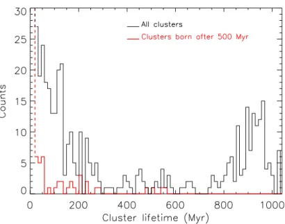
6.1 Sub-structures detected at t = 156 Myr. The diameter of the circles corresponds to the estimated size of the stellar groups. Stellar groups encompass stable clusters (or long-lived clusters, see Sect. 6.2.3) and non-persistent clusters, which will be excluded from the analysis. Note that a logarithmic scale is used for this map. . 35 6.2 Distribution of cluster lifetimes, represented for two populations: all clusters
(black thin line) and the population restricted to the clusters that form after 500 Myr (red thick line). The first bin (dashed line) goes up to 331 and 51 clusters respectively. . . 38 6.3 Mass curves of two massive clusters. The “initial mass” of the cluster is defined
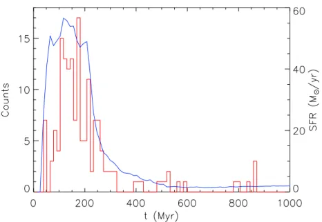
as the mass reached at the end of the growth phase, before the cluster enters the phase of steady mass evolution (see dotted line). This period generally corresponds to the first 100 Myr of cluster evolution. . . 38 6.4 Number of clusters (red) and SFR (blue) as a function of time. The absence of
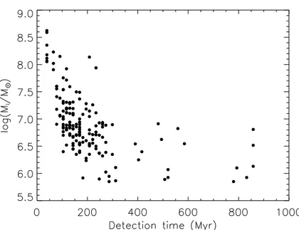
new clusters after 850 Myr results from the criteria defined to select stable clusters. 39 6.5 Distribution of the stable cluster population, in the initial mass versus detection
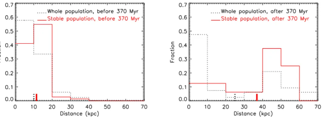
time plane. . . 40 6.6 Radial distribution of the clusters at their birth time (distances are taken at
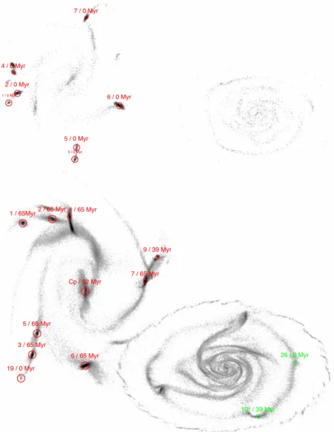
birth time), for clusters born before t = 370 Myr (left) and after t = 370 Myr (right). The stable clusters (red histograms) and whole population (dotted black histograms) are included. Average distances are marked on the distance axis. . . 41 6.7 XY projections of the spatial distribution of the young stellar component at t =
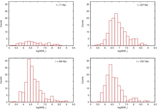
39 Myr (top) and t = 104 Myr (bottom). Massive clusters formed in the prograde galaxy (left) and in the retrograde galaxy (right) are identified with the red circles and green dashed circles, respectively. The size of each circle is proportional to the future mass gain of the cluster, with larger circles indicating a positive gain. Each cluster is labelled as follows: cluster number / age of the cluster. Cp corresponds to the nucleus of the prograde galaxy. . . 42 6.8 Cluster Mass Function at different epochs of the simulation. Each histogram
represents the average distribution over 78 Myr (6 time-steps). . . 43 6.9 Mass–Size relation for a sample of 163 stable clusters. Masses and sizes are taken
125 Myr after the first detection of the structures. The corresponding histograms of the masses and radii are also shown. The choice of 125 Myr is justified by the interval of variation of the growth phase duration. Using time shifts within the 100− 150 Myr range does not change significantly the mass–size distribution. . . 45 6.10 Mass curves of the massive clusters belonging to the prograde galaxy (top) and the
retrograde galaxy (bottom). Only the clusters not affected by boundary effects are represented. The individual clusters are labelled with an ID number. . . 45 6.11 Evolution of the kinematic parameters of the 15 most massive clusters. They are
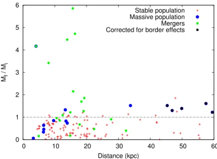
divided in two initial mass intervals. Note that vrot is plotted with a logarithm scale. The green curves represent the average trend while the red ones represent Cluster 108, the only massive sub-structure formed in-situ in tidal tails, and which may qualify as a TDG. . . 47 6.12 Cluster mass evolution as a function of the distance to the remnant. Mi(Mf,
re-spectively) is the cluster mass at the beginning (end, rere-spectively) of the simulation. 49 6.13 [Top] Same as Fig. 6.7, but at t = 234 Myr. An asterisk next to the cluster
ID, means that the cluster was missed at this time step and was identified by eye. [Bottom] Projections of two typical cluster orbits: Cluster 2 belongs to the retrograde galaxy (green dashed line), Cluster 26 belongs to the prograde galaxy (red solid line). The numbers along the prograde orbit denote times in Myr. . . . 50
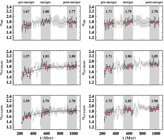
6.14 Half-mass radius, rh, versus stellar mass of our sample of simulated stable clusters 125Myr after their detection. The corresponding histograms are plotted along each axis. Observed dynamically hot stellar objects from the compilation made byMisgeld & Hilker (2011) have been added on the diagram. Clusters that are potentially affected by resolution effects have not been shown. They are however represented in the histogram of rhencompassing the area highlighted in red. The red arrow represents a possible direction for the evolution of the clusters affected by tidal disruption and experiencing a mass loss of 99 per cent. . . 52 6.15 Evolution of the power law index of the simulated CMF (top) and the CLF for
the F814W (middle) and F435W (bottom) filters. The red crosses, together with the numbers displayed above, represent the median values over interaction phases indicated by the shaded areas. Left panels take into account all the clusters whereas right panels exclude the youngest clusters (i.e., those that appeared over the past 13 Myr) (adapted fromMiralles et al.,2012). . . 54 6.16 Global Cluster Formation Rate (black histogram) and Destruction Rate (red
his-togram) as a function of time. The Stable CFR is shown in green whereas the blue line shows the Global SFR (adapted from Miralles et al., 2012). . . 55 7.1 Evolution of the SFR and the velocity dispersion of the gas in a simulation of a
galaxy merger (Bournaud et al., in prep.). . . 61 7.2 Probability Distribution Function (PDF) of the local 3D density in simulations
of discs (left) and mergers (middle), measured in 1 kpc regions around star-forming knots. Increased turbulence in mergers leads to an excess of dense gas (> 104cm−3). Derived variations of the SFR/H i and SFR/H2ratios are indicated. Interestingly, they show variations higher for SFR/H i than SFR/H2. Right: computed 2D surface density PDF of a merger simulation compared to an isolated disc. . . 62 7.3 The Schmidt-Kennicutt relation as seen by numerical simulations. The
evolu-tion of the SFR and gas surface densities of several regions of simulated colliding galaxies are plotted as a function of the merging sequence, from the initial phases (LTG discs) to the post merger phase (ETG spheroids). Adapted from Powell et al., 2012, in prep. . . 63 8.1 Examples of uv–coverage by the D-array (left), C-array (middle) and B-array
(right) configurations of the JVLA. Each segment of this plane, symmetric with respect to the origin, corresponds to the uv–components measured by one baseline. The length of each segment is a function of the duration of the observations. . . 69 8.2 Representation of the synthesised beam in 2 dimensions (left) and along a slice
including the peak (right). Note the presence of low-level oscillating wings in the response of the interferometer, known as side-lobes. . . 70 8.3 Spectral response of a VLA (left) and EVLA (right) antenna in amplitude gain
(bottom) and phase (top). The amplitude gain is normalised by the value of the channel 0, the phase is computed relatively to a reference antenna. For the reference antenna (or for a phase-calibrated baseline), the phase is set to zero across the baseband. The channel width and reference velocity are that of IF1 of NGC 7252 observations (see Table 8.1). . . 72 8.4 Image of data affected by solar interference (Arp 245) . . . 79
8.5 Input power (calibrated in units of Jy) received in the various baselines of the interferometer, as a function of the distance in the uv–domain (expressed in kilo-wavelength). The input power corresponds to channel 0 data, taken during the 2.5h the solar interference was the strongest. . . 80 8.6 Spatial distribution of the integrated H i flux in NGC 7252 (Natural weights, 20.008×
15.003 resolution). A robust-weight map (15.003× 13.006 resolution) of the spatial distribution of the integrated H i in the TDG NGC 7252NW is also displayed in the top left corner of the figure. . . 84 8.7 Spatial distribution of the integrated H i flux in Arp 245 (Natural weights, 11.0066×
7.0092 resolution). A robust-weight map (7.0017× 4.0076 resolution) of the spatial distribution of the integrated H i in the TDG Arp 245N is also displayed in the top left corner of the figure. Note the two “branches” in the north tail. They correspond to different parts of the tidal tail along the line-of-sight. Thanks to the high spatial resolution of the data, we are able to disentangle them. . . 85 8.8 Spatial distribution of the integrated H i flux in Arp 105 (Natural weights, 10.0019×
9.0065 resolution). A robust-weight map (7.0012× 7.0003 resolution) of the spatial distribution of the H i seen in absorption is also shown for the central regions. . . 86 8.9 (a) Spatial distribution of the integrated H i velocity in NGC 7252. Note the
overall velocity gradient along the tidal tails. (b) Spatial distribution of the H i velocity around the TDG NGC 7252NW (delimited by the dotted square in the top figure). The change in velocity is due to rotation locally, associated with the TDG. In both figures, density contours at 0.2 M pc−2, 1.0 M pc−2and 2.0 M pc−2 of a 2100 resolution map have been overlaid in grey. . . 87 8.10 (a) Spatial distribution of the integrated H i velocity in Arp 245. Note the overall
velocity gradient along the tidal tails. The rotation of the South West companion can be clearly seen. (b) Spatial distribution of the H i velocity around the TDG Arp 245N, delimited by the dotted rectangle in panel (a). In both figures, density contours at 1.5 M pc−2, 4.0 M
pc−2 and 9.0 M pc−2 of a 3000 resolution map have been overlaid in grey. . . 89 8.11 (a) Spatial distribution of the integrated H i velocity in Arp 105. Note the overall
velocity gradient along the tidal tails. (b) Spatial distribution of the H i velocity around the TDG Arp 105N, delimited by the dotted rectangle in panel (a). In both figures, density contours at 0.5 M pc−2, 1.5 M pc−2 and 5.0 M pc−2 of a 2100resolution map have been overlaid in grey. . . . . 91 8.12 (a) Spatial distribution of the integrated H i velocity dispersion in NGC 7252.
Note that the colour scale follows a square root progression. The velocity disper-sion appears quite heterogeneous across the system, with extreme values (above 100 km s−1) at the base of the North West Tail. (b) Spatial distribution of the ve-locity dispersion around the TDG NGC 7252NW (delimited by the dotted square on the top figure). In both figures, density contours at 0.2 M pc−2, 1.0 M pc−2 and 2.0 M pc−2 of a 2100 resolution map have been overlaid in grey. . . 92 8.13 (a) Spatial distribution of the integrated H i velocity dispersion in Arp 245. Note
that the colour scale follows a square root progression. The velocity disper-sion appears quite heterogeneous across the system, with extreme values (above 100 km s−1) in the vicinity of the central galaxies. (b) Spatial distribution of the velocity dispersion around the TDG Arp 245N, delimited by the dotted rectangle in panel (a). In both figures, density contours at 1.5 M pc−2, 4.0 M pc−2 and 9.0 M pc−2 of a 3000 resolution map have been overlaid in grey. . . 94
8.14 (a) Spatial distribution of the integrated H i velocity dispersion in Arp 105. Note that the colour scale follows a square root progression. The velocity disper-sion appears quite heterogeneous across the system, with extreme values (above 100 km s−1) in the vicinity of the central galaxies. (b) Spatial distribution of the velocity dispersion around the TDG Arp 105N, delimited by the dotted rectangle in panel (a). In both figures, density contours at 0.5 M pc−2, 1.5 M pc−2 and 5.0 M pc−2 of a 2100 resolution map have been overlaid in grey. . . 96 9.1 Optical image of Arp 245 taken with the NTT (Duc et al.,2000), combining B, V
and I bands. . . 98 9.2 Optical image of Arp 105 taken with the MegaCam on CHFT, combining B, V
and R bands (courtesy Jean-Charles Cuillandre) . . . 100 9.3 Optical image of NGC 7252, combining B and R bands (Source ESO/MPI 2.2m/WFC).
The two tidal tails are clearly visible on optical images: the Eastern Tail (ET) and the Northwestern Tail (NWT). . . 102 9.4 Location of the interacting systems on the SK-relation. The integrated values of
the total gas, H i+H2plus helium contribution (large squares), the molecular gas, H2plus helium contribution (small squares), and SFR within R25are plotted. The dashed line shows the locus of regular star-forming galaxies, whereas the dotted line corresponds to the starburst sequence, as defined byDaddi et al.(2010b). . . 104 9.5 NUV emission of Arp 245, ranging from the 3σ-level to 10 [µJy per pixel]. The
linear resolution of the NUV map is 4.5 kpc. Cyan circles locate the star-forming regions we selected and the apertures we used to measure the NUV fluxes. The diameter of the circles corresponds to 4.5 kpc. Squares locate the central galaxies of the system. H i contours, drawn from a 2100 resolution map, have been overlaid in green at 1 M pc−2, 5 M pc−2 and 9 M pc−2. . . 106 9.6 NUV emission of Arp 105, ranging from the 3σ-level to 10 [µJy per pixel]. The
linear resolution of the NUV map is 4.5 kpc. Cyan circles locate the star-forming regions we selected and the apertures we used to measure the NUV fluxes. The diameter of the circles corresponds to 4.5 kpc. Squares locate the central galaxies of the system. H i contours, drawn from a 3000 resolution map, have been overlaid in green at 1 M pc−2, 3 M pc−2 and 5 M pc−2. . . 107 9.7 NUV emission of NGC 7252, ranging from the 3σ-level to 10 [µJy per pixel]. The
linear resolution of the NUV map is 4.5 kpc. Cyan circles locate the star-forming regions we selected and the apertures we used to measure the NUV fluxes. The diameter of the circles corresponds to 4.5 kpc. A square locates the merger rem-nant. H i contours, drawn from a 2100 resolution map, have been overlaid in green at 1 M pc−2, 2 M pc−2 and 3 M pc−2. . . 108
9.8 Comparison between FUV and NUV fluxes of our sample of star forming regions in interacting systems. The data were all taken at the same linear resolution, 4.5 kpc, and fluxes were averaged over 4.5 kpc apertures and corrected for extinc-tion (internal and foreground Galactic). The 2.5σ-detecextinc-tion limits of the FUV data (NUV data) are represented by a vertical (horizontal) dotted line, for each system. The 2.5σ-detection limits for Arp 245 fall below 10−8Jy, and hence be-yond the plotting range. The NUV flux limits for the other two systems are virtually identical. Clipping at 2.5σ was applied to each system and each tracer, apart the FUV emission of Arp 105 for which the statistics of photons was too low to allow a determination of the noise level in the 4.5 kpc resolution map. Instead, the noise of the FUV data of Arp 105 was determined in a 12.5 kpc resolution map then estimated for a 4.5 kpc resolution one. . . 109 9.9 Distribution of the NUV/H i ratio across NGC 7252, at 4.5 kpc resolution. A
logarithmic scale was used for the colour coding, such that the highest value of the ratio is 5 dex higher than the smallest value. Density contours at 0.2 M pc−2, 1.0 M pc−2 and 2.0 M
pc−2 of a 2100 resolution map have been overlaid in grey. Regions of low gas column density can produce high values of the NUV/H i ratio. 111 9.10 Distribution of the NUV/H i ratio across Arp 245, at 4.5 kpc resolution. A
loga-rithmic scale was used for the colour coding, such that the highest value of the ratio is 2.5 dex higher than the smallest value. Density contours at 1.5 M pc−2, 4.0 M pc−2 and 9.0 M pc−2 of a 3000 resolution map have been overlaid in grey. Regions of low gas column density can produce high values of the NUV/H i ratio. 112 9.11 Distribution of the NUV/H i ratio across Arp 105, at 4.5 kpc resolution. A
loga-rithmic scale was used for the colour coding, such that the highest value of the ratio is 3 dex higher than the smallest value. Density contours at 0.5 M pc−2, 1.5 M pc−2 and 5.0 M pc−2 of a 2100 resolution map have been overlaid in grey. Regions of low gas column density can produce high values of the NUV/H i ratio, like in the South-East detached region of the map. . . 113 9.12 ΣSF R− ΣHI density relation for our sample of star forming regions in mergers.
All fluxes were corrected for internal and Galactic extinction. The size of the symbols is directly proportional to the distance of the star forming region to the central galaxy. Squares indicates the nuclei of the galaxies, for which extinction measurements were underestimated. For comparison, the data obtained by the pixel-to-pixel study of the outer discs of spiral galaxies by Bigiel et al. (2010) are plotted, together with additional data on mergers taken from the literature: Arp 158 and VCC 2062. The dashed lines represent lines of constant SFE (or constant depletion time). The vertical dotted line represents the saturation value of H i, as measured byBigiel et al.(2008) from a sample of spiral galaxies. . . . 115 9.13 Same as 9.12, but showing the sample of dwarf galaxies ofBigiel et al. (2010). . . 116 9.14 SFE-H i relation, per bin of ΣHI and distances to the central galaxy. The SFE
is defined as ΣSF R/ΣHI. Filled circles correspond to the median SFE (corrected for extinction) and mean ΣHI within each bin. The error bars represent the statistical dispersion within each bin. When the statistical dispersion is greater than the median value, the lower error bar corresponds to [median - min value]. When the bins contain only one value, the statistical dispersion is taken to be half of the SFE. The solid lines are power-law fits to the distributions of spirals and dwarfs ofBigiel et al.(2010). In both cases, the slope is∼ 0.7. Estimates of the SFE take into account the contribution of helium (factor of 1.34). . . 117
9.15 Evolution of the velocity dispersion of the H i gas as a function of merger stage. For the isolated case, a galaxy from the THINGS survey was used,NGC 628(Walter et al., 2008). The moment 2 maps of each galaxy are shown, together with the mean velocity dispersion. . . 119 9.16 Mass – σ relation in our sample of star forming regions in tidal tails of
inter-acting systems. A colour is attributed per system. The Jeans relation has been represented by a grey dashed line. . . 119 11.1 [From Braine et al. (2001)] Comparison of the H2/H i mass ratios in different
TDGs. The TDGs are sorted according to a possible age sequence. . . 127 11.2 Star Formation Efficiency versus H i surface density in our merger sample, grouped
into three bins of increasing distance to the central galaxy. Black and grey filled circles represent SFEs computed using the atomic gas component only, instead of the total gas mass. We checked the validity of this approximation for the outer regions of mergers for three star-forming regions with available CO data and thus for which we could determine the H i+H2 mass (red points). The solid line corresponds to a power-law fit to the SFE versus ΣHI relation for the H i– dominated regime that prevails in the outer discs of spirals (Bigiel et al., 2010). The slope is about∼ 0.7. The dashed horizontal lines represent various estimates of the SFE at several galactocentric radii in isolated spirals computed using the total gas (H i+H2) (Leroy et al.,2008) or H2 only (Bigiel et al., 2008). All SFEs plotted in the figure take into account the contribution of Helium (a factor of 1.34 like inBigiel et al.(2010)). . . 128 12.1 HST image (with F555 filter on WFPC2) of the TDG with H i (green) and Hα
(red) contours overlaid. The H i contours span the range 3.0− 6.0 M pc−2 in steps of 1.0 M pc−2. The Hαcontour corresponds to the 7σ detection level. The spatial resolution of the H i data is that of the Robust–weight data (the beam is shown in the bottom right corner). . . 136 12.2 Top panel: Crosscut (yellow outline) used to extract the emission lines of the
NWT. The width and the length of the crosscut indicate the pixels that were included. The outline follows approximately the shape of the tidal tail. We sam-pled and binned the data at 200 interval. We show surface densities above a level of 1 M pc−2. The cyan dashed regions represent the minimum and maximum spatial extents of the kinematic structure. Bottom panel: Position–Velocity diagram along the crosscut (grey scale) with black signal–to–noise ratio (S/N) contours overlaid at values of: 3σ, 5σ, 7σ and 9σ. The green line shows the ridge line following the emission maximum along each line of sight. The red and blue lines show the width of the line measured at 2.5σ (see text for further details). The yellow dashed line represent the large scale velocity gradient of the tidal tail. The yellow cross locates the centre of the kinematic structure associated with the TDG. The PV–diagram along an orthogonal crosscut through the centre of the TDG is presented in the bottom left corner. . . 137 12.3 PV–diagram of Hα along the same crosscut as that used for the H i component.
The yellow cross locates the centre of the kinematic structure associated with the TDG (see Fig. 12.2. The green line represents the velocity gradient, as expected from the H i kinematics (see Fig. 12.2). . . 139
12.4 Visible and dynamical masses of five recycled galaxies. Dark matter-free objects would lie on the black plain line. The error bars of NGC 5291’s objects were taken fromBournaud et al.(2007). The error bars of NGC 7252NW are associated to the most likely estimate of the dynamical mass (see text). The error bars of VCC 2062 are from Duc et al. (2000). The five galaxies define a trend for which the dark mass is about twice the visible mass (dashed line). . . 144
List of Tables
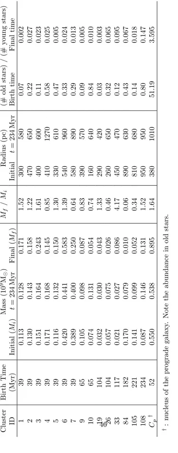
6.1 Properties of our sample of 15 massive clusters and of the nucleus of the prograde
galaxy. . . 46
8.1 NGC 7252 VLA-EVLA observations . . . 73
8.2 Arp 245 VLA observations . . . 74
8.3 Arp 105 VLA observations . . . 75
9.1 Arp 245 properties . . . 99
9.2 Arp 105 properties . . . 101
9.3 NGC 7252 properties . . . 103
9.4 GALEX observations . . . 104
10.1 Near-IR, Mid-IR and Far-IR data available for the systems that have been con-sidered so far. . . 124
12.1 Global properties of NGC 7252 and its tidal tails . . . 135
12.2 Giraffe observing parameters . . . 138
12.3 Mass budget of NGC 7252NW, compared with the TDGs in NGC 5291 and VCC 2062142 12.4 Influence of the parameters involved in the rotation model (α, σ) on the dynamical mass. The values of the dynamical mass are expressed in percent, relatively to the value obtained with the couple (α, σ) = (1, 7 km s−1). . . 143
Part I
Chapter 1
The role of mergers in the
cosmological evolution of galaxies
Our understanding of the cosmological evolution of galaxies started with the famous Hubble sequence (Hubble,1926). From the classification of galaxies based on their morphologies, a first evolutionary scheme was established to propose possible transformations of galaxies from one morphological type to another. Once the idea that two spiral galaxies can merge and form an elliptical galaxy appeared (in particular thanks to the pioneering modelling work by Toomre 1977), a whole field of investigation on the process of galaxy mergers was opened (seeSchweizer 1996andDuc & Renaud 2012for reviews).The advent of numerical simulations in modern Astronomy triggered a great step forward. Cosmological simulations have shown how the Cold Dark Matter (CDM) component (the most abundant form of matter in the Universe) structured the Universe, from the formation of small structures by gravitational collapse, to the largest and biggest ones by mergers (Melott et al., 1983;White et al.,1987;Gramann,1988;Springel et al.,2005;Gao et al.,2005;Springel et al., 2006). This scenario of structure growth is referred to as the hierarchical scenario (Peebles, 1971). The merging of structures is a key event in this current paradigm; it explains the origin of galaxy pairs, groups, clusters, super-clusters, filaments and voids, which are observed at all redshifts in the Universe.
Although the merger of CDM halos is essential in the formation of large scale structures, it does not mean that the merger of the galaxies that populate them is the dominant event in the cosmological evolution of galaxies; this for at least two simple reasons: (1) not all the CDM halos are necessarily populated by galaxies; (2) the merger of two halos is not immediately followed by the merger of the galaxies that assembled in each of their potential wells. In other words, the galaxy merger rate depends (at least) on (1) the halo occupation distribution (see Yang et al. 2005and references therein), (2) a key timescale reflecting the cosmologically-averaged “observ-ability” of mergers (seeLotz et al. 2011and references therein); both varying with the halo mass (or galaxy mass). Unfortunately, several uncertainties enter in the treatment of the baryonic physics in galaxies (Hopkins et al., 2010b), especially in the stellar feedback, which might be responsible for the overestimation of the number of dwarf galaxies occupying low-mass halos in numerical simulations (Moore et al., 1999;Klypin et al.,1999). If stronger in small structures, feedback could exceed a “simple” effect of star formation regulation (Scannapieco et al.,2008) and suppress bulge formation in small CDM halos. In addition to this, issues arise in the determi-nation of the key timescale, mainly due to the way galaxy mergers are identified in observations.
Figure 1.1: [From Lotz et al.(2011)] Observed galaxy merger rates (dots) and theoretical pre-dictions (lines). Volume-averaged major merger rate (left panel), i.e., the co-moving number density of ongoing galaxy merger events per unit time, and fractional major merger rate (right panel), i.e., the number of galaxy merger events per unit time per selected galaxy. The theoretical predictions are in good agreement with the observed major merger rates.
Observationally, merger candidates are either identified as galaxies in close pairs (sometimes in 3-D space) or as morphologically disturbed galaxies (by visual inspection or through the use of a parameter assessing the asymmetry of the system). Ignoring simple sensitivity effects, the close pair method is biased toward early-stage mergers, whereas the morphology based method (with the identification of tidal features) suffers from observational biases (as collisional debris are of low surface brightness). This results in a great deal of confusion when trying to assess the merger rate and comparing observational studies with each other. In the end, an assumption on the the merger time must be made and the merger rate is poorly constrained. In Fig.1.1, we show one of the most up-to-date determinations of the merger rate as a function of redshift (Lotz et al., 2011). The volume-averaged major merger rate appears relatively constant over cosmic times, whereas the fractional major merger rate decreases with time. Most recent results suggest that minor mergers are a possible scenario for galaxy growth; they succeed in reproducing the charac-teristics (like size, concentration, colours) of present-day early-type galaxies (Naab et al.,2009; Kaviraj et al., 2009) and could dominate the total merger rate and contribute significantly to the stellar mass assembly of galaxies (L´opez-Sanjuan et al.,2010;Hopkins et al.,2010a;Kaviraj et al.,2010; L´opez-Sanjuan et al.,2011; Lotz et al., 2011; McLure et al., 2012; Newman et al., 2012).
Besides a morphological transformation, mergers induce enhanced star formation (Kennicutt et al., 1987) and enhanced Far Infra-Red emission (Xu & Sulentic, 1991). The enhancement can be extreme and produce a burst of star formation, the so-called “starbursts” (Sanders & Mirabel,1996;Dasyra et al.,2006), sometimes reaching values of∼ 1000 M yr−1. It turns out that, at z ∼ 0, the strong Infra-Red (IR) emission of Luminous Infra-Red Galaxies (LIRGs, with 1011L
≤ LIR = L[8− 1000µm] ≤ 1012L )1 and Ultra Luminous Infra-Red Galaxies (ULIRGs, with LIR ≥ 1012L )2 is associated with the burst of star formation that is caused
1equivalent to a SFR of 20 M
yr−1≤ SFR ≤ 200 M yr−1 2equivalent to a SFR≥ 200 M
by the interaction of two galaxies (see review bySanders & Mirabel 1996). At low redshift, all ULIRGs are merging systems (while the inverse is not true). Since LIRGs are found to domi-nate the IR-emitting galaxy population at 0.5 < z < 1 (Chary & Elbaz,2001; Le Floc’h et al., 2005; Magnelli et al., 2009) and ULIRGs at z > 1 (Chapman et al., 2005; Caputi et al., 2007; Daddi et al., 2007), the conclusion that galaxy mergers would be the dominant mode of star formation in the Universe would be tentative. Yet, the (U)LIRG(z)− merger(z) connection is far from being established at all z. Recent Herschel observations of ULIRGS at z = 2, combined with high-resolution HST observations, have revealed, through the study of their morphological and kinematic features, that a significant fraction (between 25 and 50%) of ULIRGs are in fact gas rich spirals and not the result of a merger (Kartaltepe et al., 2012). Using deep FIR ob-servations obtained with the Herschel Space Observatory, Elbaz et al. (2011) showed that the fraction of starburst galaxies represents less than 20% of the IR-emitting population, including high-z ULIRGs. The contribution of merger induced starbursts to the SFR density tends to be weak at all redshifts (Sargent et al., 2012). Then, considering that galaxies form half of their stellar content at redshifts above 1 (Marchesini et al.,2009), where the population of ULIRGs dominates, these results would suggest that the building of the stellar content of galaxies would be dominated by a “secular” mode of star-formation. Mergers would only play a minor role in the global history of star formation.
Then, if mergers do not account for the bulk of stellar mass in galaxies, why should we be interested in studying them? As we show in the next Chapter, mergers offer an environment for probing the process of star-formation and the scaling relations that result from it, like the Star Formation Rate - Gas content or Schmidt-Kennicutt relation.
Chapter 2
What can mergers tell us about
the fundamental scaling relations
of star formation?
2.1
The scaling relations of Star Formation
In recent years a number of scaling relations involving the SFR have been found:
• the SFR – Stellar Mass relation (Noeske et al.,2007;Elbaz et al.,2007;Daddi et al.,2007; Pannella et al., 2009; Gonz´alez et al., 2011), which shows a tight relation between SFR and stellar mass. At all redshift, the Specific Star Formation Rate (sSFR = SFR/Mstar) decreases with mass. This anti-correlation between sSFR and stellar mass is stronger at high–z and suggests a “downsizing” scenario (Cowie et al., 1996), in which most massive galaxies form first (at high z). The sSFR - stellar mass relation is redshift-dependent, with average sSFRs increasing with redshift.
• An IR “main-sequence” (Elbaz et al., 2011), for LIRGs and ULIRGs, which corresponds to a constant LIR/L8 µm, far–to mid–IR ratio.
• the SFR – Gas content relation, also called Schmidt-Kennicutt (SK) law (Schmidt, 1959; Kennicutt, 1998b), which relates SFR and gas density through a power law. While the pioneering work of Schmidt (1959) introduced a relation between SFR and gas volume density, Kennicutt(1998b) applied this prescription to observable surface densities1:
ΣSF R= A ΣNGas (2.1)
with ΣSF R the SFR surface density in M y−1kpc−2, ΣGas the gas surface density in M pc−2. The “Gas” refers to both the atomic and molecular components. For a sample of 61 “normal” local spiral galaxies,Kennicutt(1998b) measures N = 1.4± 0.15 and A = (2.5± 0.7) × 10−4. All the measurements are averaged over the entire spatial extent of the galactic discs. Often, the ratio ΣSF R/ΣGas is referred to as the Star Formation Efficiency (SFE), its inverse is referred to as the depletion time τdep. The median gas depletion time for the sample of spiral galaxies ofKennicutt(1998b) is found to be ∼ 2.1 Gyr2.
1In the case of a galactic disc seen face-on, the surface densities corresponds to the average gas volume density
multiplied by the thickness of the disc.
All these relations should be considered when studying the process of Star Formation. They reveal a population of “standard” systems, the spiral galaxies which experience a normal mode of Star Formation, and a population of “deviant” systems, the starbursts which, at a given Stellar Mass / 8 µm-Luminosity / Gas mass, exhibit higher SFRs than the normal galaxies. In this thesis, we will focus only on the SFR – Gas relation and will specifically treat the case of galaxy mergers.
2.2
Exploring of the SFR – Gas relation
The SK-law has been the starting point of more than to decades of intense research, testing its validity form high to low gas density environments, and across a range of linear scales, from measurements obtained by integrating the SFR and gas content over entire galaxies to detailed spatially resolved studies down to typically a few hundred parsec scales.
The comparison between starbursts and normal galaxies at low and high redshifts, revealed two sequences of star-forming systems (or “modes” of star formation):
• a sequence of normal galaxies (or long-lasting mode), traced by spiral galaxies at low (Kennicutt,1998b) and high z (Tacconi et al.,2010), and additionally by BzK galaxies at high z (Daddi et al.,2010a);
• a sequence of starburst galaxies (or rapid mode), with SFEs ∼ 10 times higher than normal galaxies, traced by ULIRGs at low z and “Hyper-LIRGs” at high z (see previous chapter), and, additionally by Sub-Millimetre galaxies at high z (Bouch´e et al.,2007).
The interpretation given to the sequences of star formation, which are shown in Fig. 2.1
is still debated. A universal tight SFR – Dense Gas3 relation is observed in all environments (Gao & Solomon, 2004a,b; Juneau et al., 2009). The origin of the double sequence might be more linked to the way low density gas is transformed into intermediate density gas (as traced by CO), before the onset of star formation — this process is dealt with in Chapter 7 (in Part
II) based on predictions of numerical simulations —, or simply the way the molecular mass is estimated from CO line observations through the XCO conversion factor, with different values taken for normal galaxies and starbursts (seeNarayanan et al.(2011), which explore the effects of gas thermodynamics on the intensity of the CO emission line, resulting in an underestimation of the inferred H2 mass in a starburst environment). It was also claimed that introducing the dynamical time-scale of the systems — rotation time-scale (Daddi et al.,2010b) or free-fall time-scale (Krumholz et al., 2009) — the two sequences of star formation can be made to follow a single ΣSF R− Σgas/τdyn sequence; this would suggest that global galactic mechanisms (setting τdyn) regulates the star formation process of the system.
Parallel to the exploration of the high gas density case, a major breakthrough in our un-derstanding of the star formation process was made with the advent of interferometers. The high angular resolution achieved by these instruments allows us to resolve individual regions of galaxies and especially to isolate star forming regions from each other. Thus, one of the main goals of “The H i Nearby Galaxy Survey” (THINGS, Walter et al. 2008) is to investigate the relation between Inter-Stellar Medium (ISM) properties and Star Formation, from a sample of 34 nearby galaxies, at a spatial resolution of 100− 500 pc and a velocity resolution of 5.2 km s−1. Combining H i data from the THINGS project and CO data from the HERACLES survey (Leroy
3The dense gas can be traced by molecules with high dipole moments like HCN (which emits a line at 3 mm),
CS and HCO+. The density of the gas traced by HCN molecules is typically 2 orders of magnitude higher than
Figure 2.1: [From Daddi et al. (2010b)] SFR density as a function of the gas (atomic and molecular) surface density. The lower solid line is a fit to local spirals and z = 1.5 BzK galaxies (slope of 1.42), and the upper dotted line is the same relation shifted up by 0.9 dex to fit local (U)LIRGs and Sub-Millimetre Galaxies.
et al., 2009) with the usual tracers of star formation,Bigiel et al.(2008) reveal the existence of two gas surface density “regimes”:
• an H i–dominated regime, generally in the outskirts of late-type galaxies or in dwarf galax-ies, with the possible presence of diffuse H i gas, where the correlation between ΣSF R and ΣGas is weak ;
• an H2–dominated regime, in the inner regions of spiral galaxies, where the correlation between ΣSF Rand ΣH2is strong, with a constant molecular gas depletion time of∼ 2 Gyr, independent of galaxy characteristics.
The existence of such gas phase regimes for star formation, with a strong relation between ΣSF Rand ΣH2(Wong & Blitz,2002;Bigiel et al.,2008), reveals that, on a local scale, the SFR is controlled by the fraction of molecular gas within each clump. Once the molecular gas is formed, its transformation into stars appears to be a uniform process, at least in standard systems (spirals / dwarfs). This relation appears as the local-scale analog of the disc-averaged relation between SFR and Gas density, presented earlier, for low and high redshift spiral galaxies. In fact,Lada et al.(2012) argue that there is a fundamental scaling relation that directly connects the local star formation process with that operating globally within a galaxy. The star formation would simply be controlled by the the amount of dense molecular gas that can be assembled within a star formation complex (irrespective of if this is in a single molecular cloud or an entire galaxy). The extreme case, on the low gas density side, of the SFR–gas relation is explored by the “LITTLE THINGS” (Local Irregulars That Trace Luminosity Extremes, The HI Nearby Galaxy Survey) project (Hunter et al.,2012), with a sample of 41 gas-rich dwarf irregular galaxies ob-served at a resolution similar to, or higher than the galaxies of the THINGS project.
In this context, we present the first investigation of the SFR – Gas relation in another “extreme” case: interacting systems (mergers). Indeed, mergers are often characterised by strong starbursts (see Chapter1) and, as a consequence, are outliers of the standard SK-law. We aim at understanding the origin of this deviation. Similarly to the recent projects that benefit from the high-resolution achieved by interferometry, we have access to the physical conditions of the ISM for star-forming regions independently, so that we can explore the H i-to-dense gas relation at all scales.
We start our investigation of the SFR–gas relation on a local scale with a sample of three mergers: Arp 245, Arp 105, and NGC 7252. We present our high-resolution JVLA data, their reduction and their analysis in Part III. Our results are discussed in Part IV in the light of the various gas phase regimes defined by Bigiel et al. (2008). Our initial sample will soon be complemented by additional high-resolution H i data (Chaotic THINGs project) and additional tracers of star formation (Chapter10presents our outlook).
As the merger is expected to have effects at all scales, from a large-scale increase of the turbulence of the system (the collision of two galaxies injects an important quantity of kinetic energy in the system and stirs the gaseous component), down to the scale of single star formation4, we also explore the consequences of the merger on the properties of the ISM via the formation of star clusters during the interaction. We present the analysis we made of the population of (Super) Star Cluster that forms in a simulation of a wet major merger in Chapter6.
4SeeElmegreen(2005) for a review on the investigation of variations of the Initial Mass Function (IMF) in
starbursts. Variations towards a top-heavy IMF in starbursts are an alternative interpretation to the sequence of starbursts, since one has to assume an IMF when deriving SFR from luminosities.
Chapter 3
Outline of the thesis and
summary of my personal
contribution
The body of the manuscript is divided in three big parts, besides the general introduction (Part
I) and conclusions (PartV). Part II
Part II presents the predictions from numerical simulations made by the Saclay group on the properties of the ISM, Star-Formation and Star Cluster Formation in mergers. This part provides the theoretical framework to the topic.
My personal technical and scientific contribution in this part is the following:
• I made the detailed analysis of the output of a numerical simulation of a wet merger, exploring the data cube at different snapshots.
• I wrote the codes that identify, track and extract the properties of the star clusters (except the routine that determine the kinematic properties of the clusters, which was implemented later-on by D. Miralles-Caballero),
• I wrote a paper, entitled “Formation and evolution of massive stellar clusters in a simulated galaxy merger: on the track of the origin of GCs, TDGs and UCDs”, presenting the pipeline of the code and the analysis of the star cluster populations that form in the simulation. This paper has been submitted to MNRAS and is presented in Chapter6),
• I contributed to the comparative study between simulations and observations, presented in Miralles-Caballero et al. (see Appendix A). This paper has also been submitted to MNRAS.
Part III
From theories and predictions we switch to observations, with Part IIIbeing devoted to the SFR-H i relation. Our H i data-set and data reduction is presented in Chapter8; the analysis is presented in Chapter9.
• the calibration of the H i data and combination with archival data and mapping of the three systems studied in this report (Arp 245, Arp 105 and NGC 7252),
• the correlation of the H i maps with the UV GALEX maps, the latter obtained from the archives,
• the analysis of the spatial evolution of the SFR-H i relation in these systems. Part IV
In Part IV, we discuss the results, observational biases, and present our perspectives: an extension of the H i survey (Chapter10and inclusion of other phase of the gas, in particular the H2 traced by CO (Chapter11), and the so-called dark gas (Chapter12).
My personal technical and scientific contribution in this part is the following:
• I performed the entire calibration and data reduction of the H i observations of the merger NGC 7252 (the Giraffe Hα observations were processed by P. Weilbacher),
• I did the complete analysis of the gas kinematics of its tidal dwarf galaxy NGC 7252NW. AS part of this, I wrote code that extracts the emission lines from the spectral data cubes and creates PV-diagrams,
• I wrote a paper, entitled “Missing baryons in Tidal Dwarf Galaxies: the case of NGC 7252”, presenting the analysis of the baryonic content of NGC 7252NW and the search for dark gas (paper to be submitted and presented in Sect.12.2),
• I prepared the observations of the follow–up project, Chaotic THINGS, i.e., defined the time repartition between the different array configurations, and entered the dynamical scheduling of the new JVLA observations with the on-line Observation Preparation Tool (OPT).
Part II
Predictions from numerical
simulations of mergers
Chapter 4
Theory of star and star cluster
formation in mergers
4.1
From star to star cluster formation
One of the main effects of mergers is to increase the gas turbulence. This cascades to all scales, having an impact on the structure of the Inter-Stellar Medium (ISM), and thus possibly on the stellar Initial Mass Function (IMF), on the maximum mass of the Giant Molecular Clouds (GMCs), thus on its ability to form massive clusters and consequently on the shape of the Clus-ter Mass Function (CMF). The connection between all these scales of inClus-terest for our study is detailed below.
Molecular gas, is generally found to have a clumpy structure and to be organised in clouds. Giant Molecular Clouds (GMCs) have dense cores but that only represents ∼ 10% of the to-tal mass and toto-tal surface of the cloud. The most massive and densest cores (10− 1000 M , n(H2) ∼ 103−4M pc−2) encompass proto-clusters, that are still embedded in dust cocoons. A breakthrough in the understanding of how star clusters form in GMCs was achieved by Lada & Lada (2003) who compiled a catalogue of nearby Galactic Giant Molecular Clouds and studied their embedded clusters. They concluded that less than 4% of the proto-clusters survive more than 100 Myr, revealing a high “infant mortality” rate. Thus most of the stars initially formed in clusters quickly disperse in the ISM. Given the high rate of cluster formation (≥ 2 clusters Myr−1kpc−2) and destruction, stars that form in clusters represent the vast ma-jority of the stars populating the disc of galaxies (Allen et al., 2007). Studying the formation of clusters, as done in Chapter 4 of this thesis, is therefore insightful for understanding star-formation in general.
The important role played by star clusters in star formation led Kroupa and collaborators (Kroupa & Weidner, 2003; Weidner & Kroupa, 2005) to propose the concept of an Integrated Galactic Mass Function (IGMF)1, i.e. the sum of all the IMFs of all the dissolved star clusters. A priori, the IGMF depends on the IMF of each cluster2, on the CMF and its evolution with 1the IGMF is simply the IMF one would determine by simply observing a field of stars. The IMF is generally
measured in star clusters, ensuring that a single age stellar population is considered.
2The IMF has for long been considered universal, with a shape ξ(m) = m−α, with a slope of 1.3 for stars
with M ≤ 0.5M and the Salpeter/Massey-slope of 2.35 for M > 0.5M stars. However, different IMFs have
time (starting with an Initial CMF, ICMF3).
4.2
Building the shape of the Cluster Mass Function
Whereas the universality of the IMF has not yet firmly proven to be wrong, the CMF shows a high variety of shapes, depending on the host of the clusters, spiral or elliptical galaxies, or their age. In particular, the young Star Clusters born in nearby mergers follow a power law mass function, of index∼ −2 (Zhang & Fall,1999; Mullan et al., 2011). The mass function of older Star Clusters, like the Globular Clusters (GCs) that are found orbiting elliptical galaxies, follows a log-normal distribution (Jord´an et al., 2007). Since the most massive elliptical galaxies are believed to originate from galaxy mergers, it is tempting to establish a temporal link between the two CMFs, stating that the Globular Cluster Mass Function is an evolved form of the Young Cluster Mass Function4.
In practise, the determination of the shape of the CMF might be affected by:
• the existence of a relation between the SFR and the maximum mass of clusters (Larsen, 2002; Weidner et al., 2004;Bastian, 2008). Mergers that often exhibit a high SFR5 form more massive clusters in absolute terms and thus offer a better sampling of the high mass end of the CMF than quiescent galaxies;
• the dependence of the CMF parameters, like the low-mass turnover and the dispersion, on host galaxy luminosity (Villegas et al., 2010).
The precise shape of the CMF and its evolution might be driven by the following effects: • the infant mortality. Whether it is mass dependent or not is still debated (Lamers et al.,
2005;Whitmore et al.,2007;Fall et al.,2009;Bastian et al.,2012);
• internal processes, such as two-body relaxation and stellar evaporation, which can cause heavy mass loss;
• environmental effects, in particular during mergers through gravitational shocks, dynamical friction and tidal fields. The tidal field is found to have a complex effect on the clusters, either disrupting them in a few billion years (Fleck & Kuhn,2003), or making them tighter bound in the case of tidal compressive modes (Renaud et al.,2008,2009).
Furthermore observations and models suggest that the global shape of the CMF might change with the large scale environment. In particular, in mergers the CMF could be top heavy, as speculated for the IMF of their stars. Arguments in favor of an excess of massive clusters in mergers, or the presence of a bi-modality in the CMF, are the following:
the environment on the IMF. Whether it could be top-heavy in the starburst regions of mergers has often been proposed but never directly confirmed.
3At a time t, the Initial Cluster Mass Function is defined as the Cluster Mass Function of only the clusters
born at t. Given that the time scale of a single cluster formation is∼ 10 Myr, the uncertainty on t is at least 10 Myr.
4Note however that a fraction of the GCs around massive galaxies might be of primordial origin, while another
one might correspond to old GCs accreted together with low-mass satellites.
5a significant fraction of them are Luminous Infrared Galaxies while all Ultra-luminous Infrared galaxies are
• the observation in colliding systems of stellar structures with masses reaching that of dwarf galaxies that are not observed in other environments: either compact ones, such as the ultra-massive Super Star Cluster (SSC) W3 in the prototypical merger NGC 7252 (Maraston et al.,2004;Fellhauer & Kroupa,2005), or more extended and gas-rich ones, located along prominent tidal tails: the Tidal Dwarf Galaxies (TDGs; Duc & Mirabel,1994;Duc et al., 1997; Duc & Mirabel, 1998; Duc et al., 2000; Hibbard et al., 2001a; Mendes de Oliveira et al.,2001;Iglesias-P´aramo & V´ılchez,2001;Temporin et al.,2003;Knierman et al.,2003; Hancock et al., 2009;Sheen et al.,2009). In Sect.12.2we present a detailed study of one TDG: NGC 7252NW.
• models accounting for the high levels of gas turbulence in mergers, that predict the for-mation of clouds with a high velocity dispersion that later collapse to form massive star clusters or dwarf galaxies, in particular in tidal tails (Elmegreen et al., 1993; Kaufman et al., 1994;Duc et al.,2004).
• models reproducing the successive mergers of clusters, leading to build-up of a central massive cluster within a few 107 years , the gradual increase of its half–mass radius and finally the formation of objects similar to dwarf-Spheroidals (dSph) or dwarf-Ellipticals (dE;Kroupa,1998). The merger of sub-clusters in turbulent molecular clouds is supported by the numerical models of Bonnell et al. (2011), Saitoh et al. (2011), and Fujii et al. (2012).
Chapter 5
Insight from numerical
simulations of mergers
How do mergers affect star-formation in galaxies? In order to understand this, one should study how each galactic component involved in the process is affected: from the low density ISM, the dense molecular clouds in which stars are born to the more evolved star-clusters. This requires multi-wavelength, multi-scale observations which are in practise difficult to acquire. Indeed, the closest major merger – the Antennae – is located at more than 20 Mpc, preventing detailed stud-ies. Furthermore, such observational data do not provide hints on the temporal evolution, unless a statistical approach is used and large samples of systems observed. Then again, one faces the lack of merging systems in the nearby Universe.
Instead, numerical simulations of mergers provide time scales, and for the most current state-of-the-art models, maps with high dynamical spatial and density ranges, allowing us to determine simultaneously the evolution of the diffuse gaseous material during the collision and that of the most compact stellar systems born during the merger. Furthermore, such models provide a 3D view, unlike observational data. This is especially a limitation in observations of mergers for which projection effects may be tricky to deal with.
Provided that the physics implemented in the numerical codes is realistic enough, simulations may provide predictions that can be checked in real systems, once adapted/converted to their limited resolution. Conversely observations may reveal the physics or initial conditions in the simulations need improvement.
5.1
Historical perspective on simulations
From the pioneering work ofToomre & Toomre(1972), in the early 1970s, numerical simulations have been continuously improving, reaching ever higher levels of realism (seeDuc & Renaud 2012 for an exhaustive review on numerical simulations of interacting systems). Toomre & Toomre (1972) showed that the formation of filaments (“tidal tails” and “bridges”) during the encounter of two spirals was caused by intense gravitational tides. This allowed one to at last understand if not reproduce the morphology of the “peculiar” galaxies that had been identified a decade earlier when a complete deep atlas of the sky became available. An evolutionary sequence sorting the interacting systems by dynamical stage, from the encounter of the galaxy discs (and the appari-tion of the tails) until their final coalescence and their merger, was proposed (Toomre,1977). A
![Figure 6.13: [Top] Same as Fig. 6.7 , but at t = 234 Myr. An asterisk next to the cluster ID, means that the cluster was missed at this time step and was identified by eye](https://thumb-eu.123doks.com/thumbv2/123doknet/2296959.24176/57.892.137.759.147.902/figure-fig-asterisk-cluster-means-cluster-missed-identified.webp)