HAL Id: hal-00795168
https://hal.archives-ouvertes.fr/hal-00795168
Submitted on 27 Feb 2013
HAL is a multi-disciplinary open access
archive for the deposit and dissemination of sci-entific research documents, whether they are pub-lished or not. The documents may come from teaching and research institutions in France or abroad, or from public or private research centers.
L’archive ouverte pluridisciplinaire HAL, est destinée au dépôt et à la diffusion de documents scientifiques de niveau recherche, publiés ou non, émanant des établissements d’enseignement et de recherche français ou étrangers, des laboratoires publics ou privés.
systems: a perturbative approach
Pascal Remy
To cite this version:
Pascal Remy. Stokes phenomenon for single-level linear differential systems: a perturbative approach. Funkcialaj ekvacioj.Serio internacia, Japana Matematika Societo, 2015, 58, pp.172-222. �hal-00795168�
di¤erential systems: a perturbative approach
P. Remy
6 rue Chantal Mauduit
F-78 420 Carrières-sur-Seine
email: [email protected]
Abstract
Given a meromorphic linear di¤erential system with an arbitrary
single level r 1, we build a regular holomorphic perturbation which
preserves the single level and we show that the Stokes-Ramis matrices of the initial system are limits of convenient products of the perturbed ones. As an application, we provide an alternative method for the e¤ective calculation of the Stokes multipliers of the initial system il-lustrated on two examples. No assumption of genericity is made on the initial system.
Keywords. Linear di¤erential system, regular perturbation, holomorphic perturbation, Stokes phenomenon, summability, Stokes multipliers
AMS subject classi…cation. 34M03, 34M30, 34M40
Introduction
Throughout the paper, we are given a positive integer r 1and we consider a linear di¤erential system (in short, a di¤erential system or a system) of dimension n 2 with meromorphic coe¢ cients of order r + 1 at the origin 02 C of the form
(A) xr+1dY
dx = A(x)Y ; A(x)2 Mn(Cfxg); A(0) 6= 0 together with a formal fundamental solution at 0
e
Y (x) = eF (x)xLeQ(1=x) where
e
F (x) 2 GLn(C[[x]][x 1]) is an invertible matrix with formal mero-morphic entries in x,
L = J M
j=1
( jInj+ Jnj)where J is an integer 2, Inj denotes the identity
matrix of size nj and where
Jnj = 8 > > > > > > < > > > > > > : 0 if nj = 1 2 6 6 6 6 4 0 1 0 .. . . .. ... ... .. . . .. 1 0 0 3 7 7 7 7 5 if nj 2
is an irreductible Jordan block of size nj, Q 1 x = J M j=1 qj 1
x Inj where the qj(1=x)’s are polynomials of
max-imal degree equal to r with respect to 1=x.
In a very general system (A), the qj(1=x)’s may be polynomials in a frac-tional power in 1=x. However, they can always be changed into polynomials in the variable 1=x itself by means of an adequate …nite algebraic extension x 7 ! x , 2 N , of the variable x. The properties in view in this paper being preserved under such algebraic extensions, we may assume, without any loss of generality, that the qj(1=x)’s read as
qj 1 x = aj;r xr aj;r 1 xr 1 ::: aj;1 x 2 x 1 C x 1 : In addition, we suppose
(0:1) eF (x) 2 Mn(C[[x]]) is a formal power series in x satisfying e
F (x) = In+ O(xr);
(0:2) the eigenvalues j satisfy 0 Re( j) < 1 for all j = 1; :::; J , (0:3) 1 = 0 and q1 0.
Such conditions are not restrictive since they can always be ful…lled by means of a meromorphic gauge transformation Y 7 ! T (x)x 1e q1(1=x)Y where
T (x)has explicit computable polynomial entries in x and 1=x (cf. [1]). Recall that conditions eF (0) = In and 0 Re( j) < 1guarantee the unicity of eF (x) as formal series solution of the homological system associated with system (A) (cf. [1]). Conditions 1 = 0 and q1 0 are for notational convenience.
The assumption “system (A) has the unique level r”is equivalent to the conditions
(0.4)
1: qj q` 0or with degree r for all j; ` 2: there exists j such that aj;r 6= 0
:
Observe that, all over the article, no restrictive assumption is made except the assumption that the given system (A) has a unique level. In particular, we never assume that the formal monodromy L is diagonal or the Stokes values aj;r are distinct.
In this paper, we are interested in regular perturbations of system (A) of the form
(A") xr+1dY dx = A
"
(x)Y with A1(x) = A(x);
where " is a holomorphic multi-parameter lying in a polydisc centered at the unit 1 := (1; :::; 1) of the C-vector space Cp+1 for a convenient p 1. Besides, we suppose that, for any value of ", system (A") has, like initial system (A), the unique level r too.
The main goal of this article is to prove that the Stokes-Ramis matrices1 of initial system (A) are limits of convenient products of the Stokes-Ramis matrices of perturbed systems (A").
In a second time, we show how this result allows to build a method for the e¤ective calculation of the Stokes multipliers of initial system (A) and we illustrate it on some examples.
1In the whole paper, we call Stokes matrices all the matrices providing the transition
between any two asymptotic solutions whose domains of de…nition overlap. The name “Stokes-Ramis matrix ” used here is reserved, according to the custom initiated by J.-P. Ramis ([5]) in the spirit of Stokes’work, to the matrices providing the transition between the sums on each side of a same anti-Stokes direction. Thereby, a Stokes-Ramis matrix is a Stokes matrix, but the converse is false in general.
The organization of the paper is as follows:
In section 1, we recall some basic de…nitions about the notions of the theory of summation, such as anti-Stokes directions, Stokes-Ramis matrices, etc..., which are needed.
In section 2, based on the geometry of the anti-Stokes directions of per-turbed system (A"), we select some Stokes matrices de…ned as …nite product of Stokes-Ramis matrices which are proved to depend holomorphically on the parameter " (theorem 2.14) and to converge to the Stokes-Ramis matrices of initial system (A) when " goes to 1 (corollary 2.15). Let us point out that such results were already obtained by the author in the case r = 1 with a more speci…c perturbation (cf. [6]).
The central point of the proof of theorem 2.14 is proved in section 3. This one is based, after rank reduction, on an adequate variant of the proof of summable-resurgence theorem for single-level systems following classical Écalle’s method by regular perturbation and majorant series which was given by the author in [7].
In section 4, we combine the general results obtained in section 2 with the results of [4, 7] to build an alternative method for the e¤ective calculation of the Stokes multipliers of eF (x). As an illustration, we develop two examples. Acknowledgement I would like here to thank Professor M. Loday-Richaud for all her comments and advice which enabled me to …nalize this article.
1
Some de…nitions and notations
For the convenience of the reader, we recall here below some de…nitions about the notions of summation theory which are needed in this paper.
Anti-Stokes directions
The anti-Stokes directions (i.e., the singular directions) of system (A) (or of the full matrix eF (x)) are the directions of maximal decay of exponentials e(qj q`)(1=x)with qj q
` 6 0. More precisely, these directions are the directions determined from 0 by the rth roots of the nonzero elements of
:=faj;r a`;r ; 1 j; ` Jg:
Indeed, according to our hypothesis (0.4) of “single level equal to r”, any polynomial qj q` 6 0 is of degree r and reads
(qj q`) 1 x = aj;r a`;r xr + o 1 xr with aj;r a`;r 6= 0:
Recall that the elements aj;r a`;r of are called Stokes values of system (A). Notice that condition a1;r = 0 implies aj;r 2 for all j = 1; :::; J .
Throughout the article, we refer as a collection of anti-Stokes directions of system (A) any set ( k)k=0;:::;r 1 2 (R=2 Z)r formed by the r directions generated by a nonzero Stokes values of (i.e., determined by its rth roots).
Summation
Given a non anti-Stokes direction 2 R=2 Z of system (A) and a choice of an argument of , say its principal determination ?
2] 2 ; 0]2, we consider the sum of eY in the direction given by
Y (x) = sr; ( eF )(x)Y0; ?(x)
where sr; ( eF )(x)denotes the uniquely determined r-sum of eF at and where Y0; ?(x) is the actual analytic function Y0; ?(x) := xLeQ(1=x) de…ned by the
choice arg(x) close to ? (denoted below arg(x) ' ?).
Recall that sr; ( eF )is an analytic function de…ned and 1=r-Gevrey asymp-totic to eF on a germ of sector bisected by and opening larger than =r.
For both practical and theoretical reasons, it is worth noting that it is often useful to rewrite sr; ( eF ) in terms of 1-sums (or Borel-Laplace sums): let us denote by eF[u](t)2 Mn(C[[t]]) with u = 0; :::; r 1 the r-reduced series of eF (x), i.e., the formal series which are uniquely determined by the relation
e
F (x) = eF[0](xr) + x eF[1](xr) + ::: + xr 1Fe[r 1](xr):
Then, all the eF[u]’s are 1-summable in the direction := r and the r-sum sr; ( eF ) is related to the 1-sums s1; ( eF[u]) by the relation
sr; ( eF )(x) = r 1 X u=0
xus1; ( eF[u])(xr):
Recall that the 1-sum s1; ( eF[u])(t) is given by the Borel-Laplace integral Z 1ei
0 b
F[u]( )e =td
where bF[u]( ) denotes the Borel transform of eF[u](t).
2Any choice is convenient. However, to be compatible, on the Riemann sphere, with
the usual choice 0 arg(z = 1=x) < 2 of the principal determination at in…nity, we suggest to choose 2 < arg(x) 0 as principal determination about 0.
Stokes phenomenon and Stokes-Ramis matrices
When 2 R=2 Z is an anti-Stokes direction of system (A), we consider the two lateral sums sr; ( eF ) and sr; +( eF ) of eF at respectively obtained as
analytic continuations of sr; ( eF ) and sr; + ( eF ) to a sector with vertex 0, bisected by and opening =r. Notice that such analytic continuations exist without ambiguity when > 0 is small enough.
The Stokes phenomenon of system (A) stems from the fact that the sums sr; ( eF ) and sr; +( eF ) of eF are not analytic continuations from each other in
general. This defect of analyticity is quanti…ed by the collection of Stokes-Ramis automorphisms
St ? : Y + 7 ! Y
for all the anti-Stokes directions 2 R=2 Z of system (A), where Y + and
Y respectively denote the sums of eY de…ned for arg(x) ' ? by Y +(x) := sr; +( eF )(x)Y0; ?(x) and Y (x) := sr; ( eF )(x)Y0; ?(x):
The Stokes-Ramis matrices are de…ned as matrix representations of the St ?’s in GLn(C).
De…nition 1.1 (Stokes-Ramis matrices)
One calls Stokes-Ramis matrix associated with eY in the direction the mat-rix of St ? in the basis Y +. We still denote it St ?.
Notice that the matrix St ? is uniquely determined by the relation
Y (x) = Y +(x)St ? for arg(x) ' ? :
2
A holomorphic perturbation
In this section, we build a regular holomorphic perturbation of system (A) which preserves the single level r 1; then, based on the geometry of the anti-Stokes directions of the perturbed system, we select some Stokes matrices de…ned as convenient …nite products of Stokes-Ramis matrices and we show, on one hand, that they depend holomorphically on the para-meter and, on the other hand, that they converge to the Stokes-Ramis matrices of initial system (A).
According to the normalization eF (x) = In+ O(xr), the matrix A(x) of system (A) reads
A(x) = J M j=1 " raj;r+ r 1 X k=1 kaj;kxr k ! Inj + x rL j # + B(x)
where Lj := jInj + Jnj denotes the j
th Jordan block of the matrix L of exponents of formal monodromy and where B(x) is analytic at the origin 0 2 C. More precisely, splitting B(x) = [Bj;`(x)] into blocks …tting the Jordan structure of L, one has
(2.1) Bj;`(x) = O(x r) if aj;r 6= a`;r O(x2r) if aj;r = a `;r :
The holomorphic perturbation of system (A) considered below acts both on the Stokes values aj;r 6= 0 (hence, a fortiori, on the set of all the Stokes values of system (A) and on the anti-Stokes directions of system (A) too) and on the analytic part B(x).
Recall that a1;r = 0 and the nonzero aj;r’s are not supposed distinct. Henceforth, we denote below by !1; :::; !p with p 1 the distinct values of the aj;r 6= 0 and we rewrite as
=f!0 := 0g [ f!k !` ; k; ` = 0; :::; p and k 6= `g:
Notice that !k !` 6= 0 for all k 6= `; hence, their rth roots determine all the anti-Stokes directions of system (A):
Throughout section 2, we shall use the following notations:
Notation 2.1 For any 2 C, > 0, 2 R=2 Z and > 0, we denote below by
D( ; ) := fx 2 C ; jx j < g the open disc in C with midpoint and radius ,
D( ; ) := fx 2 C ; jx j g the closed disc in C with midpoint and radius (= the closure in C of D( ; )),
; :=fx 2 Cnf0g ; jarg(x) j < =2g the open sector with vertex 0, bisected by direction and opening ,
D ; the set of directions determined from 0 by all the points of ; ,
; =fx 2 Cnf0g ; jarg(x) j =2g the closure of ; in Cnf0g, D ; the set of directions determined from 0 by all the points of ; .
2.1
A perturbed system
We consider below a perturbation of system (A) of the form (A") xr+1dY
dx = A "(x)Y
where
(1) the parameter " := ("1; :::; "p; "p+1) lies in a polydisc Dp := p+1 Y k=1
D(1; k) of Cp+1; precise conditions on the k’s are given below,
(2) for all " 2 Dp, the matrix A"(x) reads
A"(x) = J M j=1 " ra"j;r + r 1 X k=1 kaj;kxr k ! Inj + x rL j # + "p+1B(x) with a"j;r := !0 = 0 if aj;r = !0 !k"k if aj;r = !k and k 2 f1; :::; pg :
Notice that systems (A") depend holomorphically on the parameter " and coincide with system (A) for " = 1 := (1; :::; 1) the unit of Cp+1.
Notice also that
!k"k 2 D(!k;j!kj k) for all k = 1; :::; p:
Consequently, the radius k’s, k = 1; :::; p, being chosen so that conditions (C1) D(!k;j!kj k)\ D(!`;j!`j `) = ; for all k; ` = 1; :::; p and k 6= `, (C2) 0 =2 D(!k;j!kj k)for all k = 1; :::; p,
be veri…ed (such choices exist since the !k’s are distinct in Cnf0g for all k), system (A"
) has, for all " 2 Dp, the unique level r and has for formal fundamental solution the matrix eY "(x) = eF"(x)xLeQ"(1=x)
where e
F"(x)
2 Mn(C[[x]]) is a formal power series in x satisfying eF"(0) = In, L is the matrix of exponents of formal monodromy of initial system (A),
Q" 1 x = J M j=1 q" j 1 x Inj with q"j 1 x = a"j;r xr aj;r 1 xr 1 ::: aj;1 x 2 x 1 C[x 1].
In other words, qj"(1=x) is equal to 8 > < > : 0 if aj;r = !0 !k"k xr aj;r 1 xr 1 ::: aj;1 x if aj;r = !k and k 2 f1; :::; pg :
Observe that, like systems (A") and (A), the two formal fundamental solu-tions eY"(x)and eY (x)coincide for " = 1. Observe also that, for any " 2 Dp,
e
Y "(x) has the same normalizations as eY (x). In particular, its formal series factor eF"(x)
is uniquely determined, for all " 2 Dp, by the homological sys-tem associated with syssys-tem (A") jointly with the initial condition eF"(0) = In. Furthermore, the following condition holds for all " 2 Dp:
(2.2) aj;r = 0, a "
j;r = 0, q"j 0
aj;r = a`;r , a"j;r = a"`;r , q"j q`" :
Remark 2.2 Unlike the radius k, k = 1; :::; p, which must be chosen so that conditions (C1) and (C2) hold, no condition on the radius p+1 is imposed. In particular, we can choose it as we want.
Remark 2.3 Conclusions above on systems (A") are preserved when we re-place in conditions (C1) and (C2) the closed discs D(!k;j!kj k)by the open discs D(!k;j!kj k). Actually, the choice of the closed discs is to guarantee here that 0 is not an accumulation point for the set of nonzero Stokes values of systems (A"
) when " runs in Dp. As we shall see below, this point will play an essential role.
Let us now denote by " the set of Stokes values of system (A"). By construction, the set " is deduced from the set of Stokes values of initial system (A) by replacing each nonzero Stokes value !k !` with the nonzero element !k"k !`"` (we set "0 := 1). Hence, for all " 2 Dp,
"
=f!0 = 0g [ f!k"k !`"` ; k; ` = 0; :::; p and k 6= `g:
This relation between initial Stokes values and perturbed Stokes values has a translation in terms of anti-Stokes directions.
Lemma 2.4 Let ( k)k=0;:::;r 1 2 (R=2 Z)r be a collection of anti-Stokes dir-ections of initial system (A).
Let G(( k)) be the set of Stokes values of generating the collection ( k). Then, the image of ( k) by the perturbation is the set of all the anti-Stokes directions of systems (A"), " running in
Dp, generated by all the Stokes values !k"k !`"` 2 " while !k !` 2 G(( k)).
A more precise version of lemma 2.4 is given in section 2.3, proposition 2.9. Before, we need some geometric features of the set of perturbed Stokes values.
2.2
Singular discs and singular sectors
Let us denote by
(Dp) := [ "2Dp
"
the set of all the Stokes values of all systems (A"
) when " runs in Dp. The goal of this section is to describe some of its geometric features.
1: Singular discs of (Dp)
As seen before, the perturbation changes, for all " 2 Dp, the nonzero Stokes value !k !` 2 of initial system (A) into the nonzero Stokes value !k"k !`"` 2 " of system (A"). This brings us to the following de…nition.
De…nition 2.5 (Singular disc of (Dp))
Given a nonzero Stokes value !k !` 2 of initial system (A) (hence, k 6= `), we call singular disc of (Dp) associated with !k !` the subset D!k !` (Dp) of all the Stokes values !k"k !`"` 2
" of all systems (A") when " runs in
Dp.
Notice that the set (Dp)can be rewritten as
(Dp) = f0g [ 0 @ [ !2 nf0g D! 1 A
Notice also that the choice of closed discs in conditions (C1) and (C2) (cf. remark 2.3) implies 0 =2 D! (= the closure of D! in C) for all ! 2 nf0g.
Proposition 2.6 (Description of singular discs of (Dp))
Let !k !` 2 be a nonzero Stokes value of initial system (A). Let D!k !`
be the singular disc of (Dp) associated with !k !`. Then,
D!k !` = D(!k !`;j!kj k+j!`j `)
(we set 0 := 0).
Observe that, contrary to the discs D(!k;j!kj k) (cf. condition (C1)), some of singular discs may overlap.
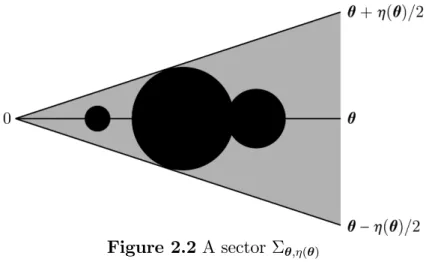
2: Singular sectors of (Dp) We denote below by
the set of all the directions determined from 0 by all the nonzero Stokes values of ,
and, for all 2 ,
the set of all the nonzero Stokes values of with argument , (Dp) :=
[ !2
D! the set of all the singular discs of (Dp)
associ-ated with ! 2 . In other words, (Dp) collects all the perturbed Stokes values of (Dp) associated with all the initial Stokes values of
determining the given direction 2 .
Figure 2.1A set (Dp)
According to proposition 2.6, all the singular discs D! with ! 2 are centered on . Then, the set (Dp)is symmetrical about . This motivates the following de…nition.
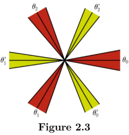
De…nition 2.7 (Singular sectors of (Dp))
Given a direction 2 , we call singular sector of (Dp) associated with the sector with minimal opening among all the sectors ; containing
(Dp). We denote it ; ( ).
Figure 2.2A sector ; ( )
Proposition 2.8 below, which states some features of ; ( ), stems from prop-erty “0 =2 D! for all ! 2 nf0g”.
Proposition 2.8 Given a direction 2 , the following properties hold: (a) ( ) < , i.e., ; ( ) is smaller than a half-plane.
(b) ( ) only depends on the radius 1; :::; p associated with the initial Stokes values !1; :::; !p. In particular, ( ) tends to 0 when the k’s go to 0.
(c) The set D ; ( ) is the set of directions determined from 0 by all the points of (Dp).
According to proposition 2.8 (b) and calculations below, we suppose, from now on, that the radius k, k = 1; :::; p, are chosen so that the following conditions be veri…ed:
(C3) for all 2 , ( ) < 2,
(C4) for all 2 , the principal determination ? of and the principal determination ( ( )=2)? of ( )=2satisfy
(C5) ; ( )\ 0; ( 0) =; for all ; 0 2 , 6= 0.
Notice that, once again (cf. remark 2.2), no condition is imposed on the last radius p+1.
We are now able to describe the action of the perturbation on the anti-Stokes directions of initial system (A).
2.3
Perturbation and anti-Stokes directions
The goal of this section is to give a precise description of the image of any collection ( k)k=0;:::;r 1 2 (R=2 Z)r of anti-Stokes directions of initial system (A) by the perturbation. To this end, we base on lemma 2.4 and on the geometric features of the set (Dp) stated in the previous section.
The main result of this section is the following proposition.
Proposition 2.9 Let ( k)k=0;:::;r 1 2 (R=2 Z)r be a collection of anti-Stokes directions of initial system (A).
Let := r 0 (hence, = r k for all k). Then, 1. 2 ,
2. the image of the collection ( k)k=0;:::;r 1 by the perturbation is the col-lection (D k; ( )=r)k=0;:::;r 1.
Recall (cf. de…nition 2.7) that ( ) denotes the opening of the singular sector of (Dp)associated with .
Recall also (cf. lemma 2.4) that, for all k = 0; :::; r 1, the directions of the set D k; ( )=r are anti-Stokes directions of systems (A
"
), " running in Dp. Proof. Obviously, is the direction determined by the Stokes values of generating the collection ( k); hence, 2 and the set G(( k)) of lemma 2.4 coincides with the set of section 2.2. Thereby, the image of ( k) is equal to the set of directions determined by the rth roots of the elements of
(Dp) (cf. lemma 2.4). Proposition 2.8 (c) ends the proof.
Observe that, like directions k’s, the sets D k; ( )=r’s are regularly
dis-tribued around the origin 0 2 C.
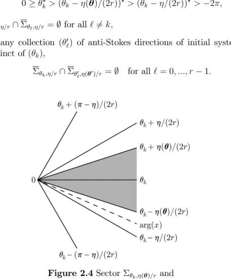
Conditions (C3) (C5) imply some obvious properties on sectors k; ( )=r which will be useful in the following calculations.
(a) For any collection ( k) of anti-Stokes directions of initial system (A),
k; ( )=r\ `; ( )=r =; for all k 6= `:
(b) For any collection ( k) of anti-Stokes directions of initial system (A), the principal determination ?
k of k and the principal determination ( k ( )=(2r))? of k ( )=(2r) satisfy
0 k? > ( k ( )=(2r))? > 2 for all k:
(c) For any two distinct collections ( k) and ( `0) of anti-Stokes directions of initial system (A),
k; ( )=r\ 0`; ( 0)=r =; for all k and `:
Figure 3 below illustrates proposition 2.10 for two collections ( k) and ( 0
`) in the case r = 3:
Figure 2.3
Remark 2.11 Proposition 2.10, (c) shows that the set (D k; ( )=r)k=0;:::;r 1
contains no other anti-Stokes directions of systems (A"
), " running in Dp, except those issuing from collection ( k) under the action of the perturba-tion. In particular, since systems (A) and (A") coincide for " = 1, the set D k; ( )=rjust contains, for all k = 0; :::; r 1, the direction kas anti-Stokes directions of initial system (A).
2.4
Initial vs perturbed Stokes-Ramis matrices
In this section, we consider a collection ( k)k=0;:::;r 1 of anti-Stokes directions of initial system (A). Let (D k; ( )=r)k=0;:::;r 1 be its image by the perturb-ation. Recall that = r k for any k (cf. proposition 2.9).
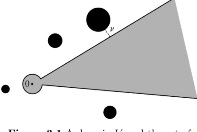
According to condition (C3) and proposition 2.10 above, there exists 2 ] ( ); =2[ such that, for all k = 0; :::; r 1,
1. k; ( )=r & k; =r & k;( )=r & k; =r;
2. the principal determination ( k =(2r))? of k =(2r) satis…es 0 k? > ( k ( )=(2r))? > ( k =(2r))? > 2 ;
3. k; =r\ `; =r =; for all ` 6= k;
4. for any collection ( 0`) of anti-Stokes directions of initial system (A) distinct of ( k),
k; =r\ 0`; ( 0)=r =; for all ` = 0; :::; r 1:
Figure 2.4Sector k; ( )=r and
associated directions
Notice that point 1. results from the choice in ] ( ); =2[ and that points 2.–4. hold as soon as is close enough to ( ). Notice also that
points 3.–4. guarantee that the set D k; =r contains no other anti-Stokes directions of systems (A"
), " running in Dp, except those of D k; ( )=r.
Let k 2 f0; :::; r 1g and …x, for now, " 2 Dp. According to points 1.–4. above, the directions k =(2r) are not anti-Stokes directions of system (A"). Thereby, (cf. section 1, page 5), the r-sums sr;
k =(2r)( eF
")are de…ned and analytic on a same germ of sector k;( )=r. Consequently, the sums
Y"
k =(2r)(x) := sr;k =(2r)( eF
")(x)xLeQ"(1=x)
are related, for arg(x) 2 k 2r ? ; k ( ) 2r ?
and x close enough to 02 C, by the relation (2.3) Y" k =(2r)(x) = Y " k+ =(2r)(x)S " ? k : The matrixS" ?
k 2 GLn(C) denotes the (perturbed) connection matrix between
Y"
k+ =(2r) and Y
"
k =(2r); it is uniquely determined by identity (2.3).
Further-more, remark 2.11 and points 1. and 3.–4. above imply that the Stokes matrix3 S"
?
k is de…ned as a (…nite) product of Stokes-Ramis matrices
as-sociated with eY " in the anti-Stokes directions of system (A") contained in D k; ( )=r. In particular, for " = 1, we have S1
? k St
?
k the Stokes-Ramis
matrix of initial system (A) associated with eY in the direction k. Indeed, Y1
k =(2r)(x) = Y k =(2r)(x) = Y k(x).
The aim of this section (and of this article) is to study the holomorphic dependence in " of the Stokes matrices S"
?
k (see theorem 2.14 below). To
this end, we must, …rst of all, answer the following questions: (a) Is there a germ k of sector
x2 C such that k 2r ? < arg(x) < k ( ) 2r ?
on which the r-sums sr;k =(2r)( eF
")
are de…ned for all " 2 Dp?
(b) If such a kexists, what can be said about the holomorphy of functions " 7 ! sr; k =(2r)( eF
")(x), x …xed in k? More precisely, are those functions holomorphic on all Dp?
As seen in section 1, page 5, we write the r-sums sr; k =(2r)( eF")(x) as (2.4) sr; k =(2r)( eF " )(x) = r 1 X u=0 xus1; =2( eF"[u])(xr)
where the eF"[u]’s denote the r-reduced series of eF". Let us admit for the mo-ment the following lemma which yields some properties on Borel transforms of the eF"[u]’s.
Lemma 2.12 Let bF"[u]( ) denote the Borel transform of eF"[u](t) with respect to t.
Let V+ (resp. V ) be a domain in C de…ned by the data of an open disc centered at 0 2 C and an open sector in C with vertex 0 and bisected by direction + =2 (resp. =2).
Suppose that the closures V + of V+ and V of V in C satisfy V +\ D! =; and V \ D! =;
for all the nonzero Stokes values ! 2 (recall that D! denotes the closure in C of the singular disc D!).
Then,
1. Domain V+
(a) For all u = 0; :::; r 1, the function ( ; ") 7 ! bF "[u]( ) is holo-morphic on V+
Dp.
(b) There exist C+; K+> 0 such that inequality b
F"[u]( ) C+eK+j j
holds for all u = 0; :::; r 1, all 2 V+ and all " 2 Dp. 2. Domain V
(a) For all u = 0; :::; r 1, the function ( ; ") 7 ! bF "[u]( ) is holo-morphic on V Dp.
(b) There exist C ; K > 0 such that inequality b
F"[u]( ) C eK j j
Observe that the existence of domains V+ and V is guaranteed, on one hand, by the fact that 0 =2 D! for all ! 2 nf0g (cf. page 10) and, on the other hand, by the fact that the choice of implies =2 =2 D 0; ( 0) for
all 0 2 (cf. points 1.–4. above).
We will prove lemma 2.12 (in fact, a stronger statement) in section 3. The following proposition gives a positive answer to questions (a) and (b) previously given.
Proposition 2.13 Let k 2 f0; :::; r 1g.
1. For all " 2 Dp, the functions x 7 ! sr; k =(2r)( eF
")(x) are all de…ned and holomorphic on the sector
k:= x2 C ; jxj < Kr and k 2r ? < arg(x) < k ( ) 2r ? where Kr := min r r 1 K ; r r 1 K+ ! .
2. For all x 2 k, the functions " 7 ! sr;k =(2r)( eF
")(x) are holomorphic on Dp.
Proof. 1. Let " 2 Dp. According to lemma 2.12, the 1-sum s1; + =2( eF"[u])(t) (resp. s1; =2( eF"[u])(t)) is de…ned and holomorphic, for all u = 0; :::; r 1, on the sector + =2 1 K+ := t 2 C ; jtj < 1 K+ and arg(t) 2 < 2 (resp. =2 1 K := t2 C ; jtj < 1 K and arg(t) + 2 < 2 ). Thereby, the choice of (cf. points 1.–4. page 15) implies that the 1-sums s1; =2( eF"[u])(t) are de…ned and holomorphic, for all u = 0; :::; r 1, on the same sector := t2 C ; jtj < K and 2 ? < arg(t) < ( ) 2 ? where K = min 1 K ; 1 K+ :
Observe that, since constants K+ and K are independent of ", sector is independent of " too. Point 1. follows from identity (2.4).
2. Fix now x 2 k. According to identity (2.4), it is su¢ cient to show that, for any u = 0; :::; r 1, the functions " 7 ! s1; =2( eF "[u])(xr) are holomorphic on Dp.
For all " 2 Dp, the 1-sums s1; =2( eF"[u])(xr)are given by the Borel-Laplace integrals s1; =2( eF"[u])(xr) = Z 1ei( =2) 0 b F"[u]( )e =xrd = Z +1 0 b G"[u]( )d where b
G"[u]( ) = bF"[u]( ei( =2))e exp(i( =2))=xr: Since ei( =2)
2 V for all 0, lemma 2.12 applies:
for all 0, the functions " 7 ! bG"[u]( ) are holomorphic on Dp, for all 0 and all " 2 Dp,
b
G"[u]( ) Fb"[u]( ei( =2)) e Re(exp(i( =2))=xr) C e (Re(exp(i( =2))=xr) K ) := M ( ):
Obviously, M does not depend on ". Furthermore, the choice “x 2 k” implying xr
2 , the functions 7 ! M ( ) are integrable on [0; +1[. Then, from Lebesgues dominated convergence theorem, the functions " 7 ! s1; =2( eF"[u])(xr) are holomorphic on Dp.
We are now able to state the two main theoretical results of this paper. Theorem 2.14 Let k 2 f0; :::; r 1g.
Then, the function " 7 ! S"?
k is holomorphic on Dp.
Proof. Let k 2 f0; :::; r 1g and x 2 k. According to proposition 2.13, 1., the Stokes matrices S"
?
k are uniquely determined, for all " 2 Dp, by the
relation (2.3) Y" k =(2r)(x) = Y " k+ =(2r)(x)S " ? k where Y" k =(2r)(x) = sr; k =(2r)( eF ")(x)xLeQ"(1=x) :
Since " 7 ! Q"(1=x)
is obvious holomorphic on Dp, proposition 2.13, 2., im-plies that the functions " 7 ! Y"
k =(2r)(x)are also holomorphic on Dp.
On the other hand, for any " 2 Dp, the matrix Y"
k =(2r) is a formal
funda-mental solution of system (A"). Thereby, Y"
k =(2r)(x) 6= 0 for all " 2 Dp
and, consequently, the functions " 7 ! Y"
k =(2r)(x)
1 are again holomorphic on Dp. Identity S"? k = Y " k+ =(2r)(x) 1Y" k =(2r)(x)
ends the proof.
Theorem 2.14 obviously leads to the following result which tells us that the Stokes-Ramis matrices St ?
k of initial system (A) are limits of the Stokes
matrices S"
? k.
Corollary 2.15 Let k 2 f0; :::; r 1g. Then,
(2.5) lim "!1S " ? k = St ? k :
Relations (2.5) will be applied in section 4 with a more speci…c perturb-ation in order to provide a method of e¤ective calculperturb-ation of the Stokes multipliers of eF (x). Before, let us end the proof of theorem 2.14 by proving lemma 2.12.
3
Proof of lemma 2.12
Recall that the formal Borel transformation is an isomorphism from the C-di¤erential algebra C[[t]]; +; ; t2 d
dt to the C-di¤erential algebra ( C C[[ ]]; +; ; ) that changes ordinary product into convolution product and changes derivation t2 d
dt into multiplication by . It also changes multi-plication by 1t into derivation dd.
Recall also that the formal Borel transform bg( ) of an analytic function g(t)2 Cftg at 0 de…nes an entire function on all C with exponential growth at in…nity.
Lemma 2.12 obviously stems from the following theorem.
Theorem 3.1 Let bF "[u]( ) denote the Borel transform of eF "[u](t) with re-spect to t.
Let V be a domain in C de…ned by the data of an open disc centered at 0 2 C and an open sector in C with vertex 0.
Stokes values ! of (recall that D! denotes the closure in C of the singular disc D! of (Dp), see section 2.2, point 1).
Then,
1. for all u = 0; :::; r 1, the function ( ; ") 7 ! bF "[u]( ) is holomorphic on V Dp,
2. there exist C; K > 0 such that inequality b
F "[u]( ) CeKj j
holds for all u = 0; :::; r 1, all 2 V and all " 2 Dp.
Notice that the existence of domain V is guaranteed by the fact that 0 =2 D! for all ! 2 nf0g (cf. page 10).
Figure 3.1 A domain V and the set of singular discs of (Dp)
The proof of theorem 3.1 is based, after rank reduction, on an adequate variant of the proof of summable-resurgence theorem for single-level systems following classical Écalle’s method by regular perturbation and majorant series which was given by the author in [7].
Remark 3.2 Since any of the column-blocks of eF"(x) associated with the Jordan structure of L (matrix of exponents of formal monodromy of system (A) and, by construction, matrix of exponents of formal monodromy of any system (A") too) can be positionned at the …rst place by means of a same
permutation P (hence, independent of ") acting on the columns of eY "(x) 4, relation
e
F"(x) = eF"[0](xr) + x eF"[1](xr) + ::: + xr 1Fe"[r 1](xr)
shows that it is su¢ cient to prove theorem 3.1 in restriction to the column-blocks ef"[u] formed by the …rst n1 (= dimension of the …rst Jordan block of L) columns of the eF"[u]’s.
3.1
Rank reduction
Let ef"(t) be the rn n1-matrix of Mrn;n
1(C[[t]]) de…ned, for any " 2 Dp, by
e f"(t) := 2 6 4 e f"[0](t) .. . e f"[r 1](t) 3 7 5 : Observe that condition eF "(x) = I
n+ O(xr) implies ef"(t) = Irn;n1 + O(t)
where Irn;n1 denotes the …rst n1 columns of the identity matrix of size rn.
By de…nition of rank reduction, the r-reduced system (A") associated with system (A"
) admits, for all " 2 Dp, a formal fundamental solution whose the …rst n1 columns of its formal series factor are equal to the n1 columns of ef"(t) (cf. [3]). Thereby, normalizations of eY "(x) (= formal fundamental solution of (A")) implies that ef"(t) is uniquely determined by the …rst n1 columns of the homological system associated with system (A")jointly with the initial condition ef"(0) = Irn;n1. This brings us to proposition 3.3 below.
Before to state it, recall that the matrix A"(x) of system (A") reads
A"(x) = J M j=1 " ra"j;r+ r 1 X k=1 kaj;kxr k ! Inj + x rL j # + "p+1B(x)
where Lj = jInj+ Jnj denotes the j
th Jordan block of L and where B(x) = [Bj;`(x)] 2 Mn(Cfxg) satis…es normalizations (2.1) Bj;`(x) = O(x r) if a" j;r 6= a"`;r O(x2r) if a" j;r = a"`;r
for all j; ` = 1; :::; J and all " 2 Dp. Recall also that 1 = a"1;r = 0 and a1;k = 0 for all k = 1; :::; r 1.
4The new formal fundamental solution reads eY"(x)P = eF"(x)P xP 1LP
eP 1Q"(1=x)P
Proposition 3.3 Let us denote by A"[u](t) (resp. B[u](t)) with u = 0; :::; r 1 the r-reduced series of A"(x) (resp. B(x)).
Then, for all " 2 Dp, the formal series ef "(t) 2 Mrn;n1(C[[t]]) is uniquely
determined by the system (3.1) rt2df
dt = A "
(t)f tf Jn1
jointly with the initial condition ef "(0) = Irn;n1, where the matrix A
" (t) 2 Mrn(Cftg) is de…ned by A"(t) = 2 6 6 6 6 6 6 4 A"[0](t) tA"[r 1](t) tA"[1](t) A"[1](t) A"[0](t) . .. ... .. . . .. . .. . .. ... .. . . .. A"[0](t) tA"[r 1](t) A"[r 1](t) A"[1](t) A"[0](t) 3 7 7 7 7 7 7 5 r 1 M u=0 utIn with A"[0](t) = J M j=1 ra"j;rInj+ tLj + "p+1B [0] (t) and A"[u](t) = J M j=1 (r u)aj;r uInj+ "p+1B [u] (t) for all u = 1; :::; r 1.
Furthermore, splitting the matrix B[u](t) = [B[u]j;`(t)] 2 Mn(Cftg) into blocks …tting the Jordan structure of L, normalizations (2.1) imply
(3.2) B[u]j;`(t) = O(t) if a "
j;r 6= a"`;r O(t2) if a"j;r = a"`;r for all u = 0; :::; r 1 and all j; ` = 1; :::; J .
Let us now denote by bf"( ) the Borel transform of ef"(t)with respect to t. In sections below, we shall prove, by applying Écalle’s method to system (3.1), that, for any domain V as in theorem 3.1,
(a) the function ( ; ") 7 ! bf"( )is well-de…ned and holomorphic on V Dp,
(b) there exist C; K > 0 such that inequality bf"( ) CeKj j holds for all 2 V and " 2 Dp.
Observe that those two points obviously lead to theorem 3.1.
Calculations below are rather similar to those detailed in [7, § 3.2] to prove the summable-resurgence theorem for single-level systems. Further-more, they generalize calculations made in [6] in the case of perturbed level-one systems.
Throughout the rest of the paper, we use the following notation.
Notation 3.4 Given a matrix M split into blocks …tting the Jordan struc-ture of L, we denote by Mj; the jth row-block of M . Thereby, Mj; is a nj p-matrix when M is a n p-matrix.
3.2
Regular perturbation
Following J. Écalle ([2]), we consider, instead of system (3.1), the regularly perturbed system
(3.3) rt2df dt = A
"
(t; )f tf Jn1
obtained by substituting B[u] for B[u] for all u = 0; :::; r 1 in the matrix A"(t) of system (3.1).
Like in [7], an identi…cation of equal powers in shows that system (3.3) admits, for all " 2 Dp, a unique formal solution of the form
e f"(t; ) = X m 0 e f"m(t) m satisfying ef"0(t) = Irn;n1 and ef "
m(t) 2 Mrn;n1(C[[t]]) for all m 1. The
following lemma yields some precisions on the ef" m’s. Lemma 3.5 Let " 2 Dp. Split ef"
m(t) = h e f"[0]m (t); :::; ef"[r 1]m (t) i into r blocks of size n n1 like ef"(t) and denote by
e f"m;j(t) := 2 6 4 e f"[0]j;m (t) .. . e f"[r 1]j;m (t) 3 7 5 for all j = 1; :::; J
the rnj n1-matrix formed by all the jth row-blocks of the ef "[u]m (t)’s (see notation 3.4).
Then, the components ef"m;j(t)2 Mrnj;n1(C[[t]]) are uniquely determined, for
all m 1 and j = 1; :::; J , as formal solutions of systems (3.4) rt2def " m;j dt A " jfe " m;j tAjfe"m;j = "p+1Bj(t)ef " m 1 tef " m;jJn1 where Bj(t) := 2 6 6 6 6 6 6 4 B[0]j; (t) tB[r 1]j; (t) tB[1]j; (t) B[1]j; (t) B[0]j; (t) . .. ... .. . . .. . .. . .. ... .. . . .. B[0]j; (t) tB[r 1]j; (t) B[r 1]j; (t) B[1]j; (t) B[0]j; (t) 3 7 7 7 7 7 7 5 is a rnj rn-matrix with analytic entries at 0 2 C and where the matrices A"j and Aj are the rnj rnj-constant matrices de…ned by
A"j := 2 6 6 6 4 ra" j;r 0 0 (r 1)aj;r 1 . .. . .. ... .. . . .. . .. 0 aj;1 (r 1)aj;r 1 ra"j;r 3 7 7 7 5 Inj and Aj := 2 6 6 6 4 0 aj;1 (r 1)aj;r 1 .. . . .. ... ... .. . . .. aj;1 0 0 3 7 7 7 5 Inj + r 1 M u=0 (Lj uInj):
Furthermore, according to normalizations (3.2), the following relations (3.5) fe"2m 1;j(t) = O(tm) and fe"2m;j(t) = O(t
m) if a" j;r = 0 O(tm+1) if a"
j;r 6= 0 hold for all m 1 and j = 1; :::; J .
Notice that the matrix A"j is invertible when a"
j;r 6= 0. Notice also that relation (2.2) implies A"j = 0 and Aj =
r 1L u=0
Lj uInj when a
" j;r = 0.
As a result of relations (3.5), the series ef"(t; ) can be rewritten as a series in t with polynomial coe¢ cients in . Consequently, ef"(t) = ef"(t; 1)
(by unicity of ef"(t) and ef"(t; 1)) and, for all , the series ef"(t; ) admits a formal Borel transform '"( ; ) with respect to t of the form
'"( ; ) = Irn;n1 +
X m 1
'"m( ) m
where '"
m( ) 2 Mrn;n1(C[[ ]]) denotes, for all m 1, the Borel transform of
e f"
m(t). In particular, the Borel transform bf"( ) reads formally as b
f"( ) = '"( ; 1) =X m 1
'"m( ) for all " 2 Dp:
The two following results give us some properties of the '"m’s. The …rst one obviously stems from lemma 3.5.
Lemma 3.6 Let " 2 Dp. Split as before '" m( ) =
h
'"[0]m ( ); :::; '"[r 1]m ( ) i into r blocks of size n n1 and denote by
'"m;j( ) := 2 6 4 '"[0]j;m ( ) .. . '"[r 1]j;m ( ) 3 7 5 for all j = 1; :::; J
the rnj n1-matrix formed by all the jth row-blocks of the '"[u] m ( )’s. Then, for all m 1, the components '"
m;j( )2 Mrnj;n1(C[[ ]]) are iteratively
determined, for all j = 1; :::; J , as solutions of systems (3.6) R" j d'" m;j d = Sj' " m;j+ d d Bcj ' " m 1 '"m;jJn1 where '"
0 := Irn;n1, cBj denotes the Borel transform of Bj and where the
rnj rnj-matrices Rj" and Sj are de…ned by
R" j = 2 6 6 6 4 r( a"j;r) 0 0 (r 1)aj;r 1 . .. . .. ... .. . . .. . .. 0 aj;1 (r 1)aj;r 1 r( a"j;r) 3 7 7 7 5 Inj and Sj = 2 6 6 6 4 0 aj;1 (r 1)aj;r 1 .. . . .. ... ... .. . . .. aj;1 0 0 3 7 7 7 5 Inj+ r 1 M u=0 (Lj (u + r)Inj).
Lemma 3.6 implies the following proposition. Proposition 3.7 Let V a domain as in theorem 3.1. Then, the function ( ; ") 7 ! '"
m( ) is holomorphic on V Dp for all m 1. Proof. Since the Bj’s are analytic at 0 2 C, their Borel transforms cBj are entire functions on all C. Consequently, normalizations (3.2) imply that the only singularities in C of systems (3.6) are the Stokes values a"j;r 6= 0 of (Dp). Proposition 3.7 follows from the fact that domain V never meets
(Dp)nf0g.
To prove theorem 3.1, we are left to show that (a) the function ( ; ") 7 ! bf"( ) = '"( ; 1) = X
m 1 '"
m( ) is well-de…ned and holomorphic on V Dp,
(b) there exist C; K > 0 such that inequality bf"( ) CeKj j holds for all 2 V and " 2 Dp.
These two points are proved below by using a technique of majorant series satisfying a convenient system. Of course, there exist many possible majorant systems. Here, we make explicit a possible one.
3.3
Majorant series
Let denote the minimal distance between the elements of V and the ele-ments of (Dp)nf0g (cf. …gure 3.1). According to condition “V \ D! = ; for all ! 2 nf0g”(cf. theorem 3.1), we have > 0.
Let g = g[0]; :::; g[r 1] be a rn n1-matrix split as previously into r blocks of size n n1. Let gj denote the rnj n1-matrix formed by all the jth row-blocks of the g[u]’s:
gj := 2 6 4 g[0]j; .. . g[r 1]j; 3 7 5 for all j = 1; :::; J: In the case where g = Irn;n1, we simply denote by I
j
Let us now consider, for j = 1; :::; J , the regularly perturbed linear system (3.7) 8 > > > > > < > > > > > : Cj(gj Irn;nj 1) = (Ir Jnj)gj+ gjJn1 2I j rn;n1Jn1 + ( p+1+ 1)jB jj (t) t g if aj;r = 0 (Rj tSj)gj = tgjJn1 + ( p+1+ 1)jBjj (t)g if aj;r 6= 0 where
jBjj (t) denotes the series Bj(t)in which the coe¢ cients of the powers of t are replaced by their module,
Cj is an invertible constant rnj rnj-diagonal matrix with positive entries which will be adequatly chosen below (see proposition 3.9), Rj and Sj are the rnj rnj-constant matrices de…ned by
Rj := 2 6 6 6 4 0 0 jaj;r 1j . .. . .. ... .. . . .. . .. 0 jaj;1j jaj;r 1j 3 7 7 7 5 Inj and Sj := 2 6 6 6 4 0 jaj;1j jaj;r 1j .. . . .. . .. ... .. . . .. jaj;1j 0 0 3 7 7 7 5 Inj + r 1 M u=0 j r u r 1 Inj+ Jnj :
Recall that j denotes the eigenvalue of the jth Jordan block Lj of L. Notice that the constant p+1+ 1 satis…es j"p+1j p+1+ 1 for all " 2 Dp. Notice also that system (3.7) depends on the domain V but not on the parameter ".
Up to the constant p+1+ 1, system (3.7) is the majorant system used in [7] to prove summable-resurgence theorem for single-level systems. Hence, by adapting calculations made in [7, § 3.2.2], we can prove the following lemma. Lemma 3.8 The Borel transformed system of system (3.7) admits, for = 1, a unique solution of the form
bg( ) = Irn;n1 +
X m 1
which is entire on all C with exponential growth at in…nity. Furthermore, using notations as above, the components m;j( )2 Mrnj;n1(C[[ ]]) of m( )
are iteratively determined, for all m 1 and j = 1; :::; J , as solutions of systems: Case aj;r = 0: Cj m;j = (Ir Jnj) m;j+ m;jJn1 + ( p+1+ 1) d d jBdjj m 1 : Case aj;r 6= 0: Rj d m;j d =Sj m;j + m;jJn1 + ( p+1+ 1) d d jBdjj m 1 : We set 0 := Irn;n1.
In particular, m( ) is an entire function on all C and lies in Mrn;n1(R
+ f g) for all m 1.
The following proposition shows that bg de…nes a convenient majorant series of the bf"’s.
Proposition 3.9 Let a be a constant such that jarg( )j a for all 2 V . Let Cj = 1 max 1 j Jexp(2ajIm jj) r 1 M u=0 1 Re j r u r Inj:
Then, for all m 1, 2 V , " 2 Dp and j = 1; :::; J , the following inequalities hold:
(3.8) '"m;j( ) m;j(j j) In particular, the series
bg(j j) = X m 1
m(j j)
is a majorant series of bf"( ) for any "2 Dp.
Proposition 3.9 is proved by applying Grönwall lemma to systems de…ning the '"m;j’s and the m;j’s. Calculations are similar to those detailed in [7, § 3.2.2] and are left to the reader. However, note that the constant K which appears in [7] is equal to 1 in our case. Indeed, according to the de…nition of domain V , the “optimal” path from 0 to any 2 V is here the straigth line [0; ].
Remark 3.10 Like system (3.7), the majorant series bg(j j) depends on do-main V but not on the parameter ". This is the key point of the proof of theorem 3.1 as we shall see in the next section 3.4.
We are now able to prove theorem 3.1.
3.4
Proof of theorem 3.1
Recall that we must prove the two following points: (a) the function ( ; ") 7 ! bf"( ) = X
m 1 '"
m( ) is well-de…ned and holo-morphic on V Dp,
(b) there exist C; K > 0 such that inequality bf"( ) CeKj j holds for all 2 V and " 2 Dp.
According to propositions 3.7 and 3.9 and remark 3.10, the series ( ; ")7 ! bf"( ) = X
m 1 '"m( )
is a series of holomorphic functions on V Dp which normally converges on all the compact sets of V Dp. Hence, point (a).
As for point (b), it stems from inequality bf"( ) bg(j j) (proposition 3.9) and from the fact thatbg has exponential growth at in…nity (lemma 3.8).
This ends the proof of theorem 3.1.
4
E¤ective calculation of Stokes multipliers
In this section, we are given a collection ( k)k=0;:::;r 1 2 (R=2 Z)r of anti-Stokes directions of system (A) and we consider, for all k, the anti-Stokes-Ramis matrix St ?
k associated with eY (x) in the direction k (cf. de…nition 1.1).
Split St ? k = [St
j;`
?
k] into blocks …tting the Jordan structure of the matrix L
of exponents of formal monodromy (hence, Stj;`?
k is a nj n`-matrix). Split
e
F (x) in the same way and denote by eF ;`(x)its `th column-block (recall that e
The matrix Stj;j?
k is the identity matrix Inj of size nj and, for j 6= `, the
matrix Stj;`?
k is zero as soon as kis not a direction of maximal decay of
expo-nential e(qj q`)(1=x). When
k is a direction of maximal decay of exponential e(qj q`)(1=x) (hence, j 6= ` and the Stokes value a
j;r a`;r generates the collec-tion ( k)), the entries of Stj;`?
k are called Stokes multipliers of eF
;`(x) in the direction k.
The goal of this section is to build a method for the e¤ective calculation of the Stokes multipliers of eF (x) based on the results of the holomorphic perturbation of system (A) stated in section 2.
As in section 3 (cf. remark 3.2), we restrict our study to the calculation of the Stokes multipliers of the …rst column-block ef (x) of eF (x). Henceforth, we denote by stj;?
k in place of St
j;1
?
k and we suppose that ( k)is a collection of
anti-Stokes directions of system (A) associated with ef (x)(otherwise, stj;? k = 0
for all k and j). Recall that such a collection ( k) is generated by (at least) one of the Stokes values !1; :::; !p (= the distinct values of the aj;r 6= 0, cf. the beginning of section 2).
4.1
Stokes multipliers and connection constants
Let denote the set of Stokes values !1; :::; !p. For any ! 2 , we call front of ! the set of polynomials qj(1=x) with leading term !=xr. According to the hypothesis (0.4) of single level equal to r, the front of ! is a singleton
! xr + _q!
1 x
where _q! 0 or _q!(1=x) is a polynomial in 1=x of degree r 1 and with no constant term. When _q! 0, the Stokes value ! 2 is said to be with monomial front. Notice that, in the case r = 1, all the Stokes values of are with monomial front.
In the two previous papers [4] (case r = 1) and [7] (case r 2), M. Loday-Richaud and the author displayed explicit formulæ between the Stokes multi-pliers of ef (x)associated with the Stokes values ! 2 5 with monomial front (hence, all the Stokes multipliers of ef (x) when r = 1) and the connection constants given, in the Borel plane, by the right analytic continuation (see [4, § 3.4] for a precise de…nition) of the Borel transforms bf[u]( ) at = !. Recall that such formulæ exist too when ! has a non-monomial front, but
require to …rst reduce ! into a Stokes value with monomial front by means of a convenient change of the variable x in initial system (A) (cf. [7, § 4.3.2]).
Thereby, the e¤ective calculation of the Stokes multipliers of ef (x)can be reduced to the e¤ective calculation of the connection constants of the bf[u]( ). As an illustration, we develop below three typical examples.
Example 4.1 Let us consider the system
(4.1) x2dY dx = 2 6 4 0 0 0 x2 1 + x 4 0 2x3 x 3 3 7 5 Y
together with the formal fundamental solution eY (x) = eF (x)xLeQ(1=x) where
Q 1 x = diag 0; 1 x; 3 x , L = diag 0;1 4; 0 , e F (x) = 2 4 1 0 0 e f2(x) 1 0 e f3(x) 1 3 5 2 M3(C[[x]]) satis…es eF (0) = I3, e f2(x) = x2 7 4x 3 + O(x3) and fe 3(x) = x3+ O(x3).
System (4.1) has the unique level 1 and =f1; 3g. Then, the direction = 0 is the unique anti-Stokes direction of system (4.1) associated with the …rst column ef (x) of eF (x). The Stokes-Ramis matrix St0 in this direction reads
St0 = 2 4 1 0 0 st2 0 1 0 st3 0 1 3 5 :
Furthermore, according to [4, thm. 4.3], the Stokes multiplier st2
0 (resp. st30) is related to the connection constant k2
1;+ (resp. k33;+) of bf ( ) at the point = 1 (resp. = 3) by the relation
(4.2) st20 = (1 + i) p 2 3 4 k1;+2 (resp. st30 = 2i k3;+3 ).
Since the formal series ef2(x) and ef3(x)satisfy the equations 8 > > > > < > > > > : x2d ef2 dx 1 + x 4 fe2 = x 2 x2d ef3 dx 3 ef3 = 2x 3+ x ef 2 ,
their Borel transforms bf2( ) and bf3( )are the unique solutions of the system 8 > > < > > : ( 1)d bf2 dx + 3 4fb2 = 1 ; bf2(0) = 0 ( 3) bf3 = 2+ 1 fb2 .
Hence, for all j j < 1, 8 > > > < > > > : b f2( ) = 4 3 4 3(1 ) 3=4 b f3( ) = 3 2+ 4 12 + 12(1 )1=4 3( 3)
(we chose a determination of the logarithm such that ln( ) 2 R for > 0). Thereby, the connection matrices K1;+ and K3;+ of bf ( )at the points = 1 and = 3 are given by
K1;+ = 2 6 6 4 0 k2 1;+= 2p2 3 (1 + i) 0 3 7 7 5 and K3;+= 2 4 0 0 k3 3;+ = 9 + 27=4(1 + i) 3 5 : Then, identities (4.2) imply
(4.3) st 2 0 = 8i 3 3 4 st30 = 2i (27=4 9 + 27=4i) :
Observe that, in this example, the choice of a triangular matrix for system (4.1) allows us to explicitly write the Borel transform bf ( )and, consequently, to calculate the exact values of the Stokes multipliers st2
0 and st30. Of course, such a case is anecdotal and, in a more general situation, i.e., for systems for which the matrices are not triangular, such exact calculations are not possible anymore. Nevertheless, we can always determine an approximation of the connection constants hence, of the Stokes multipliers by using a technique of successive analytic continuations like shown below.
Example 4.2 Let us now consider the system (4.4) x2dY dx = 2 6 6 4 0 0 x x 1 + x 2 0 0 x 2 + x 3 3 7 7 5 Y
together with the formal fundamental solution eY (x) = eF (x)xLeQ(1=x) where
Q 1 x = diag 0; 1 x; 2 x , L = diag 0;1 2; 1 3 , e F (x) 2 M3(C[[x]]) satis…es eF (x) = I3+ O(x).
As in example 4.1, system (4.4) is a level-one system and = 0 is its unique anti-Stokes direction associated with the …rst column ef (x) of eF (x) (we have
=f1; 2g). The Stokes-Ramis matrix St0 reads
St0 = 2 4 1 0 0 st2 0 1 0 st30 1 3 5
and, according to [4, thm. 4.3], the Stokes multiplier st20 (resp. st30) is related to the connection constant k2
1;+ (resp. k2;+3 ) of bf ( )at the point = 1 (resp. = 2) by the relation (4.5) st20 = 2p k21;+ (resp. st30 = ( p 3 + i) 2 3 k2;+3 ). Let ef (x) = 2 6 4 e f1(x) e f2(x) e f3(x) 3 7
5. Since the efj’s are formal series solutions of the system 8 > > > > > > > > > > < > > > > > > > > > > : x2d ef1 dx = x ef3 x2d ef2 dx 1 + x 2 fe2 = x ef1 x2d ef3 dx 2 + x 3 fe3 = x ef2 ,
their Borel transforms bfj’s satisfy the di¤erential equations 8 > > > > > > > > > > > < > > > > > > > > > > > : d bf1 d = fb1+ bf3 ( 1)d bf2 d = bf1 1 2fb2 ( 2)d bf3 d = fb2 2 3fb3 .
Consequently, the Borel transform bf ( ) = 2 6 4 b f1( ) b f2( ) b f3( ) 3 7 5 of ef (x) is an analytic solution on the open disc D(0; 1) of the system
(4.6) dZ d = 2 6 4 1 0 1 1 1 1 2( 1) 0 0 12 3(22) 3 7 5 Z
which has two regular singular points at = 1 and = 2. More precisely, system (4.6) reads near = 1 as
(4.7) ( 1)dZ d = C1( 1)Z with C1( ) := 2 6 4 +1 0 +1 1 12 0 0 1 3(2 1) 3 7 5 and near = 2 as (4.8) ( 2)dZ d = C2( 2)Z with C2( ) := 2 6 4 +2 0 +2 +1 2( +1) 0 0 1 2 3 3 7 5 : Notice that C1( 1) is analytic on the open disc D(1; 1) and C2( 2) is analytic on the open disc D(2; 1). Following Wasow ([8]), we consider the two matrices D1 := 2 4 1 0 0 2 1 0 0 0 1 3 5 and D2 := 2 4 1 0 0 0 1 0 0 32 1 3 5
so that M1 := D11C1(0)D1 = diag 0; 1 2; 0 and M2 := D21C2(0)D2 = diag 0; 0; 2 3 .
Hence, choosing as before a determination of the logarithm such that ln( ) 2 R for > 0, system (4.7) (resp. system (4.8)) has for fundamental solution at = 1 (resp. = 2) a matrix of the form
Z1( 1) = D1G1( 1)( 1)M1 (resp. Z2( 2) = D2G2( 2)( 2)M2)
where G1( 1) 2 M3(Cf 1g) (resp. G2( 2) 2 M3(Cf 2g)) is analytic on the open disc D(1; 1) (resp. D(2; 1)) and satis…es G1(0) = I3 (resp. G2(0) = I3). More precisely,
the …rst and the third columns of Z1( 1)are analytic on D(1; 1); the second column of Z1( 1)reads as
2 4 0 ( 1) 1=2 0 3 5 + ( 1)1=2g1( 1) with g1( 1)analytic on D(1; 1),
the two …rst columns of Z2( 2) are analytic on D(2; 1); the third column of Z2( 2) reads as 2 4 0 0 ( 2) 2=3 3 5 + ( 2)1=3g2( 2) with g2( 2)analytic on D(2; 1).
Following Cauchy’s theorem, the right analytic continuation of bf (still de-noted bf) at the point = 1 (resp. = 2) is a solution of system (4.7) (resp. system (4.8)). Thereby, there exists a unique matrix
S1 := 2 4 1 1 2 1 3 1 3 5 2 M3;1(C) (resp. S2 := 2 4 1 2 2 2 3 2 3 5 2 M3;1(C))
such that bf ( ) = Z1( 1)S1 for all 2 D(1; 1)nf1g (resp. bf ( ) = Z2( 2)S2 for all 2 D(2; 1)nf2g). In particular, calculations above shows that the connection constant k2
1;+ (resp. k32;+) is equal to 12 (resp. 32), and, consequently, identities (4.5) imply
st20 = 2p 12 and st30 = ( p 3 + i) 2 3 3 2:
We are left to evaluate 2
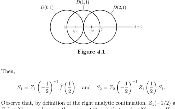
1 and 23. According to the geometry of the “conver-gence discs”D(0; 1), D(1; 1) and D(2; 1) (see …gure 4.1 below), we evaluate, on one hand, bf ( )and Z1( 1)at the point = 1=2and, on the other hand, Z1( 1)and Z2( 2)at the point = 3=2.
Figure 4.1 Then, S1 = Z1 1 2 1 b f 1 2 and S2 = Z2 1 2 1 Z1 1 2 S1:
Observe that, by de…nition of the right analytic continuation, Z1( 1=2) and Z2( 1=2) are evaluate at the point 1=2such that arg( 1=2) = . Hence, one can check that
2 1 0:46823766i 3 2 3:05123307 + 2:39083857i and, consequently, st20 1:6598593i st3 0 6:714284368 + 16:68631306i :
This method by successive analytic continuations still holds for systems with a single arbitrary level r 2. However, the calculations may be much more di¢ cult when one of the singular points of generating the collection ( k) is with non-monomial front.
Example 4.3 Here below, we consider the system
(4.9) x3dY dx = 2 6 4 0 0 x2 x2 1 + x 0 0 x2 2 + x 2 2 3 7 5 Y
together with the formal fundamental solution eY (x) = eF (x)xLeQ(1=x) where
Q 1 x = diag 0; 1 2x2 1 x; 1
x2 (hence, the system has the unique level 2, = f1=2; 1g and the front of 1=2 (resp. 1) is non-monomial (resp. monomial)),
L = diag 0; 0;1 2 , e
F (x) 2 M3(C[[x]]) satis…es eF (x) = I3+ O(x2).
As before, we denote by ef (x) the …rst column of eF (x). We also denote by e
f[u](t) with u = 0; 1 the 2-reduced series of ef (x).
Let ( 0 = 0; 1 = ) be the unique collection of anti-Stokes directions of system (4.9) associated with ef (x). For all k 2 f0; 1g, the corresponding Stokes-Ramis matrix St k reads
St k = 2 4 1 0 0 st2 k 1 0 st3 k 1 3 5 :
We are just interested below in the calculation of the Stokes multipliers st3
k’s
associated with the Stokes value with monomial front 1. According to [7, cor. 4.5], the st3
k’s are related to the connection constants k
[u]
1;+ of bf[u]( ) at the point = 1 by the relations
8 > > > > > > > > > < > > > > > > > > > : st30 = (1 + i) p 2 3 4 k1;+[0] (4 4i) 3 4 k [1] 1;+ st3 = ( 1 + i) p 2 3 4 k[0]1;++ (4 + 4i) 3 4 k [1] 1;+ :
To determine an approximation of the k1;+[u] ’s, we can proceed, like in ex-ample 4.2, by a method of successive analytic continuations. According to proposition 3.3, e f(t) := " e f[0](t) e f[1](t) # 2 M6;1(C[[t]])
is a formal series solution of the system
2t2dY dt = 2 6 6 6 6 6 6 4 0 0 t 0 0 0 t 1 0 0 t 0 0 t 2 +2t 0 0 0 0 0 0 t 0 t 0 1 0 t 1 t 0 0 0 0 0 t 2 2t 3 7 7 7 7 7 7 5 Y:
By adapting calculations of previous example 4.2, one can check that the Borel transform bf( )of ef(t)is an analytic solution on the open disc D(0; 1=2) of the system (4.10) dZ d = 2 6 6 6 6 6 6 6 4 1 0 1 2 0 0 0 1 2 1 2 2 1 0 0 1 2 1 0 0 2(1 1) 4(3 1) 0 0 0 0 0 0 23 0 21 1 (2 1)2 2 (2 1)2 0 1 2 1 2(3 2) (2 1)2 0 0 0 0 0 1 2( 1) 5 4( 1) 3 7 7 7 7 7 7 7 5 Z
which has an irregular singular point at the Stokes value with non-monomial front = 1=2and a regular singular point at the Stokes value with monomial front = 1. More precisely, system (4.10) reads near = 1 as
(4.11) ( 1)dZ
d = C1( 1)Z
where C1( 1)is the analytic matrix on the open disc D(1; 1=2) de…ned by
C1( ) := 2 6 6 6 6 6 6 6 4 +1 0 2( +1) 0 0 0 2 +1 2 2 +1 0 0 2 +1 0 0 1 2 3 4 0 0 0 0 0 0 2( +1)3 0 2( +1) (2 +1)2 2 (2 +1)2 0 2 +1 2 (3 +1) (2 +1)2 0 0 0 0 0 12 54 3 7 7 7 7 7 7 7 5 .
As in example 4.2, we consider the matrix D1 := 2 6 6 6 6 6 6 4 1 0 0 0 0 0 0 1 0 0 0 0 0 23 1 0 0 0 0 0 0 1 0 0 0 0 0 0 1 0 0 0 0 0 25 1 3 7 7 7 7 7 7 5 so that M1 := D11C1(0)D1 = diag 0; 0; 3 4; 0; 0; 5 4 .
Then, system (4.11) has a fundamental solution of the form Z1( 1) = D1G1( 1)( 1)M1 where G1( 1) 2 M6(Cf 1g) is analytic on the open disc D(1; 1=2) and satis…es G1(0) = I6 (cf. [8]). More precisely,
the third column of Z1( 1) reads 2 6 6 6 6 6 6 4 0 0 ( 1) 3=4 0 0 0 3 7 7 7 7 7 7 5 + ( 1)1=4g1;3( 1) where g1;3( 1)is analytic on D(1; 1=2), the sixth column of Z1( 1)reads
2 6 6 6 6 6 6 4 0 0 0 0 0 ( 1) 5=4 3 7 7 7 7 7 7 5 + ( 1) 1=4g1;6( 1) where g1;6( 1)is analytic on D(1; 1=2),
the four other columns of Z1( 1)are analytic on D(1; 1=2).
= 1 is a solution of system (4.11), there exists a unique matrix S1 = 2 6 6 6 6 6 6 4 1 1 2 1 3 1 4 1 5 1 6 1 3 7 7 7 7 7 7 5 2 M6;1(C)
such that bf( ) = Z1( 1)S1 for all 2 D(1; 1=2)nf1g. Thereby, the connection constants k1;+[0]3 and k
[1]3
1;+ are given by k[0]31;+ = 13 and k1;+[1]3 = 16. The two constants 3
1 and 61 can be numerically evaluate in a similar way as example 4.2 by considering the analytic continuation of bf from the disc D(0; 1=2) (= the disc of convergence of bf( )) to the disc D(1; 1=2) (= the disc of “convergence”of Z1( 1)) through any disc of the form D(1=2 ia; a) with a > 0.
Figure 4.2
Notice that, for any a > 0, the point = 1=2 ia is an ordinary point of system (4.10); hence, any of its fundamental solution is analytic on the disc D( ; a). Notice also that the choice of such a disc is due to the fact that we must bypass the irregular singular point = 1=2 of system (4.10) to the right to connect D(0; 1=2) and D(1; 1=2).
The two previous examples 4.2 and 4.3 bring us to the following general remark.
Remark 4.4 Let ( k)be a collection of anti-Stokes directions of system (A) associated with the …rst column-block ef (x) of eF (x). Let us assume that this collection is generated by s 2 Stokes values of , say !1; !2; :::; !s with j!1j < j!2j < ::: < j!sj.
Fix ` 2 f2; :::; sg and suppose that !` has a monomial front (recall that such a condition can always be ful…lled by means of a convenient change of the variable x in system (A)). Then, as shown in examples 4.2 and 4.3 above, the connection constants of the bf[u]( )’s at !` can be evaluate as follows:
(a) evaluate all or part of the connection constants at the intermediate Stokes values !1; :::; !` 1 who have a monomial front,
(b) bypass all or part of the intermediate Stokes values !1; :::; !` 1 to the right (always those with a non-monomial front and possibly the others). With a numerical point of view, these two methods pose some problems. Indeed, point (a) requires to handle fundamental solutions at regular singular points (see example 4.2) and their numerical evaluations are much more di¢ cult than those of fundamental solutions at ordinary points. As for point (b), if it allows to avoid handling fundamental solutions at regular singular points as point (a) by focusing on fundamental solutions at ordinary points, it signi…cantly increases the number of intermediate numerical evaluations which can degrade the precision of the results obtained (see example 4.3).
In section 4.2 below, we build an alternative method for the e¤ective cal-culation of Stokes multipliers in order to get around all these di¢ cults. This method is based on a perturbation of system (A) in which each perturbed Stokes value generates its own collection of anti-Stokes directions.
4.2
E¤ective calculation and perturbation
We consider here below a collection ( k) of anti-Stokes directions of system (A) associated with the …rst column-block ef (x) of eF (x). As previously, we denote by the set of nonzero Stokes values !1; :::; !p of system (A) associated with ef (x). We also denote by (k) the set of Stokes values of
generating the collection ( k).
The goal of this section is to build a method for e¤ective calculation of the Stokes multipliers of ef (x) in the directions k, k = 0; :::; r 1, when the cardinal ] ( k) of ( k) is 2 (hence, p 2too).
4.2.1 Case of two Stokes values 1. Setting the problem
In this section, we suppose ] ( k) = 2, i.e., just two Stokes values of , say
!1 and !2, generate the collection ( k). We also suppose, without loss of generality, that j!1j < j!2j.
Then, as collection of anti-Stokes directions of the full matrix eF (x), the collection ( k)is generated by the three Stokes values !1, !2 and !2 !1 and possibly by the Stokes values of the form
!j !k with !j 2 ( k), !k 2= (k) and arg(!k) = r 0
or of the form
!j !k with !j; !k 2= ( k), i.e., distinct of !1 and !2
if they exist.
2. A perturbed system
Let us now …x > 0 and let us consider, for all " 2 [0; ], the system (A") in which the initial Stokes value !2 of system (A) is replaced by !2e ir". Let " denote the set deduced from by replacing !2 by !2e ir" too. Then, for all " 2 [0; ], "is the set of nonzero Stokes values of system (A")associated with the …rst column-block ef"(x)of eF"(x)(we resume the perturbed notations as section 2).
Observe that, for small enough, the set of systems (A")"2[0; ] de…nes a sub-perturbation P (A) of the holomorphic perturbation of system (A) studied in section 2. In particular, the image of ( k) by P (A) is a subset of (D k; ( )=r)k=0;:::;r 1 (cf. proposition 2.9) and corollay 2.15 tells us that the corresponding Stokes matricesS"
?
k (see page 16) tend, for all k = 0; :::; r 1,
to the initial Stokes-Ramis matrices St ?
k when " goes to 0.
Lemmas 4.5 and 4.6 below allow us to precise this last result by making explicit the image of ( k) by P (A) as well as the form of the matrices S"?
k.
Lemma 4.5 (Action of P (A) on the collection ( k))
Given " 2 [0; ], the collection ( k) of initial system (A) splits into the fol-lowing collections of anti-Stokes directions of system (A"):
1. the collection ( k) which is generated by the Stokes value !1 and possibly by all the Stokes values of the form !1 !k with arg(!k) = r 0 or of the form !j !k with !j; !k 2= ( k) if they exist,