HAL Id: hal-01085208
https://hal.archives-ouvertes.fr/hal-01085208
Submitted on 20 Nov 2014
HAL is a multi-disciplinary open access
archive for the deposit and dissemination of
sci-entific research documents, whether they are
pub-lished or not. The documents may come from
teaching and research institutions in France or
abroad, or from public or private research centers.
L’archive ouverte pluridisciplinaire HAL, est
destinée au dépôt et à la diffusion de documents
scientifiques de niveau recherche, publiés ou non,
émanant des établissements d’enseignement et de
recherche français ou étrangers, des laboratoires
publics ou privés.
location-routing problem
Nathalie Bostel, Mi Zhang, Pierre Dejax
To cite this version:
Nathalie Bostel, Mi Zhang, Pierre Dejax. A new model for the capacitated single allocation hub
location-routing problem. 5th International Conference on Information Systems, Logistics and Supply
chain, Aug 2014, Breda, Netherlands. �hal-01085208�
A new model for the capacitated single allocation
hub location-routing problem
Nathalie Bostel
a, Mi ZHANG
b, Pierre Dejax
ca L’UNAM Université, Université de Nantes, IRCCyN UMR CNRS 6597,
58 rue Michel Ange, B.P.420, 44606 Saint-Nazaire, France
b
L’UNAM Université, École Centrale de Nantes, IRCCyN UMR CNRS 6597, 1 rue de la Noë, B.P.92101, 44321 Nantes, France
c
L’UNAM Université, École des Mines de Nantes, IRCCyN UMR CNRS 6597, 4 rue Alfred Kastler, B.P.20722, 44307 Nantes, France
Email: [email protected], [email protected], [email protected]
Abstract—We address the problem of designing a logistic system for general goods transport firms to ship goods from many origins to many destinations through routing and con-solidation via hubs. To that purpose we propose a new model for the hub location-routing problem (HLRP). This problem considers the location of hub facilities concentrating flows for less-than-truckload (LTL) shipments together with the design of both collection and distribution routes associated with each hub. Very few published works directly address the HLRP and it is focused on particular cases such as the postal services. Our mathematical model focusses on the capacitated fixed cost HLRP with single allocations (CSAHLRP). We have developed a set of instances inspired by the Australian Post (AP) data set. Extensive experiments using a standard solver prove the good performance of our model for solving small to medium size problems.
Keywords: Transportation, Hub location-routing prob-lem, less-than-truckload shipments
I. INTRODUCTION
With the increasing pressure for performance of logistics systems in terms of reduction of costs and time for delivery while reducing the shipment loads, less than truckload (LTL) shipments get more and more attention, especially for the goods-transport industry (fresh food, drinks or parts) and postal service providers. In logistic systems of LTL shipments, an LTL carrier collects cargoes from various origins (i.e. shippers, producers) via collection tours or directly and consolidates them for shipment to the destinations (i.e. clients, retail stores) via one or several hubs. After collection, the freight is sorted and consoli-dated in the hub either for additional line-hauls to another hub terminal or for shipment to the destinations either directly or through delivery tours (Barnhart et al. 2002). In some cases such as postal services, collections and deliveries may be done simultaneously. In other cases such as refrigerated freight carriers, collections and deliveries are organized separately. For example, in this LTL service case, collections from shippers are made in the afternoon while deliveries to clients are made in the next morning, to allow inter-hub transportation overnight with fully loaded long-haul trucks.
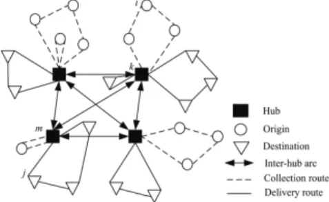
Therefore, the performance of the LTL system is not only related to the distance between origins and destinations but is also dependent on the design of the network of hub terminals and the efficiency of transportation routing operations. In order to design an efficient LTL shipment network with the objective of minimizing the total cost and meeting the required delivery times, companies need to determine the location of the hubs, the allocation of origins (shippers) and destinations to the hubs, and the optimal collection and delivery routes within the network. This problem is known as the hub location-routing problem (HLRP) and addressing it is the goal of this paper. The objective is to minimize the total cost of the system, including fixed costs to establish hubs, inter-hub trans-portation costs, and collection/delivery routing costs. An example of the HLRP is shown in Figure 1 where the circles, the triangles and the squares represent the origins of goods, the destinations and the hubs, respectively. The bold edges represent the transfer arcs connecting hubs. The dashed edges represent the local collection arcs connecting non-hub terminals to one hub while the simple solid edges are the local delivery arcs. In this paper, we focus on the case where the collections and deliveries are made separately. Therefore we distinguish two kinds of tours (collection and delivery tours).
Figure 1. The network of the hub location-routing problem
As can be understood from the above description, the HLRP is related to two classic optimization problems: the hub location problem (HLP) and the location-routing problem (LRP). The HLP involves the location of hub
facilities concentrating flows in order to take advantage of economies of scale and through which flows are to be routed from origins to destinations. For an extensive review on the HLP, ones can refer to Alumur & Kara (2008) or Campbell & O’Kelly (2012). The goals of the LRP are to determine the locations of the depots, the allocation of customers to depots, and to design the distribution (or collection) routes in a system based on distribution of goods from warehouse to destinations, or collection the other way. Nagy & Salhi (2007) presented a survey on issues, models and methods for the LRPs. In their classification, they pointed out a particular case of the LRP where inter-facilities routes are considered and both pick-up and delivery routes must be determined: this refers to the many-to-many location-routing problem (MMLRP) that is similar to the HLRP. Different from the LRP which only considers one type of routes, the HLRP considers both collection and distribution routes. Clearly, the HLRP considers all the decisions associated with the HLP and the LRP. Thus, in this paper, we focus on modeling and solving the HLRP, assuming that the collections and deliveries are handled separately and that fixed costs for establishing hubs and operating vehicles are considered. Based on the literature review, the aims of this paper are to analyse the state of the art, propose a mathematical model for the capacitated single alloca-tion HLRP (CSAHLRP) and validate it with instances inspired by the Australian Post (AP) data set (Ernst & Krishnamoorthy 1999). Based on the above description, the subsequent parts of this paper are organized as follows. Section 2 describes the state of the art of the HLRP. Then the notations and a mathematical formulation of the HLRP are presented in Section 3. Section 4 introduces the computational experiments. Conclusions and prospects are given in Section 5.
II. STATE OF THE ART
In contrast to the HLP and the LRP, which have been the subject of much research, only very few works have directly addressed the HLRP. Nagy & Salhi (1998) in-troduced a mathematical formulation and a two-stage heuristic for the many-to-many location-routing problem (MMLRP) which is very similar to the HLRP but in the specific context of postal service applications. For the MMLRP, they combined the facility location problem and the vehicle routing problem with pickup and delivery activities that may occur simultaneously. They proposed a "locate first and routing second" heuristic to solve this problem, but only one instance was solved and the results were limited. Liu et al. (2003) studied a mixed truck delivery system that allows both hub-and-spoke and direct shipment delivery modes. They introduced a heuristic al-gorithm to determine the delivery mode for each supplier-customer pair and to perform vehicle routing with two modes. The experimental results showed that this mixed system can save traveling distance, compared with the two
pure systems. Though the system considers pickup and delivery routing in a hub-and-spoke network, it includes only one hub. It can therefore be treated as a 1-HLRP with direct shipment.
In addition, some researchers have focused on the partitioning-hub location-routing problem (PHLRP) which is a hub location problem involving graph partitioning and routing features. Özsoy et al. (2008) first introduced three integer programming formulations of the PHLRP and compared them to identify which one performed best. Catanzaro et al. (2011) explored possible valid inequalities to strengthen the IP model and introduced a branch-and-cut algorithm to solve the PHLRP which contains 20 vertices. Ta et al. (2012) presented a binary integer linear programming model and a new method based on the difference of convex function algorithms to solve larger problems with up to 25 vertices.
The hub location-routing problem has also been applied to postal service network problems which assumed that the pickup and delivery could occur simultaneously. Wasner & Zäpfel (2004) developed a two-layer hub location and vehicle routing model for an Austrian parcel delivery ser-vice. In their non-linear model, they considered the number of trips between hubs, the quantity transferred between depots directly or across hubs, the number of pickup and delivery routes, and the capacity of vehicles. To solve this non-linear model, a heuristic solution concept was introduced based on a sequence of local search procedures to determine the number and location of hubs and depots, and their assigned service areas as well as the routes. However, these authors studied only one case to illustrate their solution concept. Çetiner et al. (2010) developed a two-stage method that includes locating and routing for an uncapacitated-length-limited HLRP for the Turkish postal delivery system. The heuristic contains hubbing and routing stages which iterate during the whole procedure using an updating scheme of the distance used in the first stage. A case study for the Turkish postal service with 81 nodes was developed and tested to prove the effectiveness of this model and method. More recently, de Camargo et al. (2013) proposed a new formulation and a tailored Benders decomposition algorithm for the many-to-many hub location-routing problem (MMHLRP) of a parcel delivery network consisting of locating the hubs, generating local tours to service the non-hub nodes and connect the non-hub nodes to the installed hubs, and routing the flow. In this formulation, it is assumed that the pickups and the deliveries may occur simultaneously and that a constraint for each local tour limits the maximum time allowed. In the proposed algorithm, the formulation was divided into the master problem to provide a lower bound (LB) and the subproblem to provide an upper bound (UB) to obtain an optimal solution. Computational results based on the AP standard data set confirmed the efficiency and robustness of the algorithm which can solve instances of up to 100 nodes.
Today, more and more researchers consider incorporating the routing cost into the location problem. In the 20th EWGLA, Martín et al. (2013) presented a mixed integer programming formulation and proposed a branch-and-cut algorithm for the hub-cycle location problem (HCLP). In their model, they considered the cycle routing costs in the single allocation p-hub location problem and assumed that the pickups and the deliveries could be done simul-taneously. In addition, they assumed that each hub could operate one route at most and that each route was limited to the maximum number of nodes. In the same conference, Kartal et al. (2013) presented a mathematical mini-max model which considered the integration of uncapacitated single allocation p-hub center and multi depot multiple traveling salesman problems. The goal of the model was to minimize maximum route lengths without capacity. And then two heuristics based on simulated annealing and random descent were introduced and tested on CAB, AP and Turkish data sets. In TRISTAN 2013 (Eighth Triennial Symposium on Transportation Analysis), Lüer-Villagra et al. (2013) presented a formulation model for the p-hub location and vehicle routing problem for which they proposed two exact solution approaches (branch-and-cut and Benders decomposition). Their model is also based on the postal delivery system. Computational experiments were performed on the AP data set ranging from 10 nodes to 25 nodes with CPLEX.
In summary, most of the studies on the HLRP have focused on postal systems in which no vehicle capacity is taken into account and where collection and delivery may be done in the same tours. There is a lack of models addressing the HLRP for general goods shipments. So, to the best of our knowledge, our research is the first in which a model is proposed to the capacitated single allocation hub location-routing problem (CSAHLRP) for general goods shipment and where the collection and delivery occur independently and flows are concentrated through hubs.
III. MATHEMATICAL FORMULATION AND DEFINITION
Because the HLRP is a combinatorial optimization prob-lem related to the HLP and the LRP, the proposed model is based on two classic formulations of these problems. One is the mixed integer linear programming formula-tion developed by Ernst and Krishnamoorthy (Ernst & Krishnamoorthy 1999) for the capacitated single allocation hub location problem (CSAHLP), and the other one is a mathematical formulation given by Wu et al. (Wu et al. 2002) for the multi-depot location-routing problem. These two formulations were selected because of their reduced number of variables or constraints. In this section, we develop a mathematical model for the capacitated single allocation hub location-routing problem defined in the introduction.
We consider a complete graph G = (N, E) with a vertex set N = H ∪ I ∪ J , where H is the set of potential
hubs, I is the set of suppliers (origins) and J is the set of clients (destinations). Associated with the network G, a distance matrix is defined, where the elements dij are
the distance between two nodes (i, j) ∈ E, i ∈ N, j ∈ N . We consider also a demand matrix with elements qij
being the flow quantity for each supplier-client pair, where i ∈ I, j ∈ J . So, in order to route the flow from suppliers to clients, the network can be viewed as a set of three components: the collection process from suppliers to hubs, the transfer process between hubs and the delivery process from hubs to clients. Parameters α, β and γ reflect the unit costs for the transfer, collection and delivery processes, respectively. In this model, the transportation cost between hubs (α) depends on the distance and the flow quantity transferred while the routing costs for the local collection and delivery tours (β and γ) only depend on the distance of the arcs traversed as it is usually assumed. In addition to the above transportation costs, we consider fixed costs for operating hubs and vehicles. Let Γk be the capacity and
Fk the fixed cost of hub k. For the vehicles, we consider
a homogeneous fleet with a capacity Q and a fixed cost fv.
Based on the above description, the CSAHLRP model allows one-hub-stop or two-hub-stops for each supplier-client pair rather than the direct connection. Moreover, as the activities of collection from suppliers and delivery to clients are considered separately, a supplier and a client cannot be allocated to the same local tour. In this model, the number of hubs required is not imposed and will result from the optimization, taking into account the capacity restrictions and fixed costs for potential hubs. In addition, each origin or destination (O-D) node will be allocated to one open hub and one vehicle (single allocation). According to these hypotheses, the CSAHLRP needs to decide which candidate hub will be open and to assign each supplier and client to only one hub. At the same time, for each hub-suppliers group or hub-clients group, the optimal routes will be designed. So, the decision variables in this model are defined as follows:
Ykli− the fraction of flow from supplier i passing from hub k to hub l;
zik− the allocation variable of a node i to a hub k. It
is equal to 1 if the node i is allocated to the hub k, 0 otherwise; specially, zkk = 1 if the hub k is selected to
be open; xv
ij− the routing variable equals 1 if the arc (i, j) is
served by vehicle v, 0 otherwise.
Besides the above parameters and variables, additional notations used in this model are presented below:
N − the set of all nodes, N = H ∪ I ∪ J ; V − the set of vehicles v ∈ V ;
Oi− the total quantity of flow originating at supplier i,
Oi=Pj∈Jqij;
Dj− the total quantity of flow destined to client j, Dj=
P
i∈Iqij;
To clarify the presentation of the model, we divide the constraints into four parts: the hub location constraints; the collection routing constraints; the delivery routing constraints and the constraints on the values of variables. Then, based on the above definitions, the mathematical formulation of the CSAHLRP is presented as follows:
M inX k∈H Fkzkk+ X i∈I X k∈H X l∈H αdklOiYkli +X v∈V X i∈I∪H X j∈I∪H,j6=i βdijxvij+ X v∈V X i∈J ∪H X j∈J ∪H,j6=i γdijxvij +X v∈V X k∈H X i∈I∪J fvxvki (1) subject to
—hub location constraints:
zik≤ zkk ∀i ∈ N, ∀k ∈ H (2) X k∈H zik= 1 ∀i ∈ I ∪ J (3) X i∈I Oizik≤ Γkzkk ∀k ∈ H (4) X j∈J Djzjl ≤ Γlzll ∀l ∈ H (5) X l∈H Ykli = zik ∀i ∈ I, ∀k ∈ H (6) X l∈H YlkiOi= X j∈J qijzjk ∀i ∈ I, ∀k ∈ H (7)
—collection routing constraints:
X i∈I∪H X j∈I Ojxvij ≤ Q ∀v ∈ V (8) X i∈I∪H xvij− X i∈I∪H xvji= 0 ∀v ∈ V, ∀j ∈ I ∪ H (9) X u∈I∪H (xvku+ xvui) ≤ 1 + zik ∀i ∈ I, ∀k ∈ H, ∀v ∈ V (10) X v∈V X i∈I∪H xvij = 1 ∀j ∈ I (11) X i∈H X j∈I xvij≤ 1 ∀v ∈ V (12) X i∈H X j∈I X v∈V xvij ≥ d P i∈I P j∈Jqij Q e (13)
—delivery routing constraints: X i∈J ∪H X j∈J Djxvij ≤ Q ∀v ∈ V (14) X i∈J ∪H xvij− X i∈J ∪H xvji= 0 ∀v ∈ V, ∀j ∈ J ∪ H (15) X u∈J ∪H (xvku+ xvuj) ≤ 1 + zjk j ∈ J, ∀k ∈ H, ∀v ∈ V (16) X v∈V X i∈J ∪H xvij = 1 ∀j ∈ J (17) X i∈H X j∈J xvij≤ 1 ∀v ∈ V (18) X i∈H X j∈J X v∈V xvij ≥ d P i∈I P j∈Jqij Q e (19)
—constraints on values of variables:
Uiv− Ujv+ |I|xvij≤ |I| − 1 ∀v ∈ V, ∀i ∈ I, ∀j ∈ I
(20) Uiv− Ujv+ |J |xvij ≤ |J | − 1 ∀v ∈ V, ∀i ∈ J, ∀j ∈ J (21) X i∈H X j∈H xvij = 0 ∀v ∈ V (22) 0 ≤ Ykli ≤ 1 ∀i ∈ I, ∀k ∈ H, ∀l ∈ H (23) zik∈ {0, 1} ∀i ∈ N, ∀k ∈ H (24) xvij∈ {0, 1} ∀i ∈ N, ∀j ∈ N, ∀v ∈ V (25) Uiv ≥ 0 ∀i ∈ I ∪ J, ∀v ∈ V (26)
The objective function minimizes the sum of the fixed hub costs, transportation cost between hubs, collection routing cost, delivery routing cost and fixed costs of vehicles. Constraints (2) indicate that a spoke is allocated to an open hub. Constraints (3) show that an O-D node is allocated to only one hub (single allocation). Constraints (4) and (5) are hub capacity constraints for collection and delivery. Constraints (6) and (7) are the flow conservation equation at the hubs. They show that if an O-D node is allocated to a hub, then all the flow from or to the node should pass through this hub. The above constraints are related to the hubs and their allocations. Constraints (8)-(13) are collection routing constraints. Constraints (8) are the vehicle capacity constraints. Constraints (9) are the flow conservation constraints. Constraints (10) provide the connection between location variables and routing variables. They specify that a supplier can be assigned to a hub only if there is a vehicle from that hub go-ing through that supplier. Constraints (11) ensure that a supplier can only be served by one vehicle. Constraints (12) guarantee that each vehicle can be used once at
most for collection routing. Formulas (13) are generalized valid inequalities from capacitated vehicle routing problem which limit the minimum total number of vehicles used for collection. Here, dxe denotes the smallest integer not less than x. Equations (14)-(19) are the delivery routing constraints, which have similar meanings to the collection routing constraints. Constraints (20) and (21) are sub-tour elimination constraints for the collection and delivery routing. Constraints (22) prohibit collection or delivery routes between hubs. Constraints (23)-(26) are constraints on the values of variables.
IV. COMPUTATIONAL EXPERIMENTS AND RESULTS
In this section we show the results of our computational experiments carried out on a set of randomly generated instances inspired by the AP data set introduced by Ernst and Krishnamoorthy (Ernst & Krishnamoorthy 1999). Because none are directly available in the literature for the CSAHLRP, so first, we describe the generation of instances of different sizes.
A. Test instances and parameter setting
The standard AP data set can produce instances ranging from 10 to 200 nodes with a generator. In the initial instances, it includes the coordinates of nodes, the hub capacity, the hub fixed cost and the flow quantity between nodes. However, it does not include the vehicle capacity and its fixed cost. Because our HLRP considers collections and deliveries separately, also needs to distinguish the set of potential hubs, suppliers and clients. Here, we generate two classes of test sets including 16 small and medium instances based on different criteria (see Table 2). We set the fixed cost at 20,000 Euros for each hub and 2,000 Euros for each vehicle. Following some initial evaluations, the parameter α (inter-hub cost) has been set to 0.8e/km.loading unit and parameters β and γ are set to 2 and 3e/km respectively. The distances dij are set to
the Euclidean distance between two nodes.
The first class of test sets contains 5 HLRP instances inspired by the AP data set with capacitated hubs and vehicles. In this set, the number of suppliers and clients ranges from 10 to 20 whereas the number of candidate hubs ranges from 3 to 6. For each instance, the coordinates of suppliers are those of the AP data set. As the client set is identical to the supplier set in the AP, we generate our client set coordinates {(xj, yj)|j ∈ J } by applying
a linear transfer xj = x 0
j + 10000, yj = y 0
j + 10000
based on the original data set. Here, (x0j, yj0) is the initial coordinates of node j in the AP data set. We thus obtain two "clustered" sets of nodes, one for the suppliers and one for the clients. We then generate 3 or 6 potential hubs randomly from the set of suppliers and clients coordinates. We consider two types of vehicle (large and small: L and S). The small capacities are calculated based on the maximum quantity of flow associated with a supplier or a client, to ensure feasibility regarding the single allocation
and single visit constraints. The large ones are set to twice the small ones. In the same way, we define two categories of hub capacities (large and small: L and S). The small ones are generated to ensure that the total flow of all nodes can be handled and one hub can accommodate at least two small vehicles. The large ones are set to twice the small ones. Thereby, for each instance, we obtain four variants depending on the capacities of hubs and vehicles. The data of the first class of instances are detailed in Table 1, where the following notation is used to name the instances: H − I − J , representing the number of potential hubs, the suppliers and the clients, respectively. About the size of these instances, we distinguish them with the number of suppliers. The small instances consider a number of suppliers from 5 to 15 and the medium ones have 20 suppliers. The capacity values (L/S) of hubs and vehicles are shown in columns 3 and 4 of Table 1.
TABLE 1
DESCRIPTION OF THE FIRST CLASSES OF INSTANCES
AP inspired
Class 1 Hub capacity (loading unit) Vehicle capacity (loading unit) 3-10-10 6000/3000 2400/1200 3-15-15 4500/2250 1800/900 3-20-20 5000/2500 2000/1000 6-10-10 1000/600 300/250 6-20-20 5000/2500 2000/1000 TABLE 2
DESCRIPTION OF THE SECOND OF INSTANCES
AP inspired
Class 2 Hub capacity (loading unit) Vehicle capacity (loading unit) 3-5-5 2620 1179/917/655 3-10-10 2232 1005/782/558 3-15-15 368 166/129/92 3-20-20 1416 638/496/354 3-25-25 340 153/119/85 6(10)-10-10 1640 738/574/411 6(10)-15-15 1500 675/525/375 6(10)-20-20 1224 551/429/306
The second class test set is composed of 11 instances also inspired from the AP data set with three different vehicle capacity parameters. For these instances, the number of suppliers and clients remain identical to the first class set but the numbers of hub candidates generated increases from 3 and 6 to 10. In this second class set, the coordinates of suppliers and clients are selected randomly from the AP data sets and then 3, 6 and 10 potential hubs are selected, also randomly, from the supplier and client sets. For example, the initial 10-nodes AP instance can generate the HLRP instances 3-5-5, the initial 20-nodes instance can generate the HLRP instances 3-10-10, 6-10-10 and 10-10-10, and so on. Whenever, the coordinates of one supplier/client couple are the same, the flow is set at 0, because, here, this kind of flow is assumed to needn’t be transported through a hub. For the capacities of hubs and vehicles, in order to test the effect of different vehicle
capacities, we use this formula: Q = 2 ∗ Vpara which
ensures that each hub can receive at least two vehicles. Here, the different values of Vpara are set at 0.9, 0.7
and 0.5 as suggested in Wu et al. (2002). Then the hub capacities Γ of the second class are obtained using the formula: Γ = max{ P i∈IOi |H| , 4 ∗ max{Oi, Dj|i ∈ I, j ∈ J }} (27) where |H| is the number of potential hubs. This formula compares two values and uses the largest one for the hub capacity. The first one represents the average capacity of all potential hubs to ensure that the global capacity can handle the total flow quantity. The second one is four times the maximum quantity of flow associated with a supplier i or a client j. The choice of these values ensures feasibility of the class 2 data set regarding the single route allocation constraints even with the smallest vehicle capacity (Vpara = 0.5). The values of the hub capacities
and vehicle capacities are shown in the last two columns of Table 2. From Table 2, it can be seen that the number of potential hubs generated increases gradually with the different instances.
To evaluate the quality of our model, it was coded in the C++ language and solved with solver CPLEX 12.5 on all of the above instances. All computational experiments were conducted on an Intel Core i3 CPU of 2.93 GHz and 6 GB of memory, running on the operational system Window 7. Here, the running time for CPLEX is limited in three hours. All the results are presented in Tables 3-4.
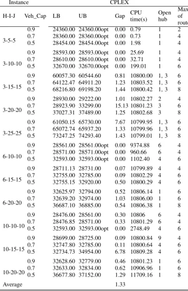
B. Performance analysis of the experimental results Tables 3 and 4 present the results obtained by CPLEX for all small and medium instances from the two classes of test sets. Here, the optimal solution is reported if it is reached before the time limit or a feasible solution otherwise. The best lower bound found is also reported if the time limit is reached. In these two tables, the instance names indicate the number of candidate hubs, suppliers and clients while the letters "L" and "S" denote the capacity of hubs and vehicles in Table 3. For example, the instance "3-10-10LS" in Table 3 refers to an instance with 3 candidate hubs, 10 suppliers and 10 clients, with a large capacity for hubs, and a small capacity for vehicles. The "Veh_Cap" column in Table 4 indicates the parameter used to calculate the capacity of vehicles. To show the results obtained by CPLEX, the following notations are used in Tables 3 and 4.
NFS: no solution found by CPLEX because of lack of memory;
LB: lower bound or best lower bound found by the CPLEX;
UB: the upper bound found by CPLEX in a limited time, marked "opt" if the solution is optimal; GapLB: the deviation in % of the upper bound
from the lower bound found by the CPLEX. Here,
GapLB= LB × 100%;
CPU time(s): running time in seconds used for CPLEX;
Open hubs: the index of the located hubs;
Max of routes: the maximum number of routes assigned to a hub for collection and delivery together in the optimal or best solution.
TABLE 3
EXPERIMENTS RESULTS OBTAINED BYCPLEXON INSTANCES OF
CLASS1
Instance LB UB GapLB CPUtime(s) Openhub Max of routes 3-10-10LL 28599.00 28599.00opt 0.00 111.43 3 4 3-10-10LS 36841.00 36841.00opt 0.00 6005.35 3 8 3-10-10SL 55595.50 57368.80 3.19 10799.93 1, 2 2 3-10-10SS 63777.20 63904.00 0.20 11011.32 1, 2 6 3-15-15LL 32847.00 32847.00opt 0.00 7199.84 3 6 3-15-15LS 40984.30 41094.00 0.27 10799.86 3 10 3-15-15SL 61685.20 62527.00 1.36 10800.17 1, 2 4 3-15-15SS 69862.60 70908.80 1.50 10800.15 1, 2 6 3-20-20LL 28829.50 28982.00 0.53 10802.8 2 4 3-20-20LS NFS 3-20-20SL 61210.22 87702.00 43.28 10799.95 2, 3 2 3-20-20SS 69480.09 74881.00 7.77 10799.84 2, 3 6 6-10-10LL 32653.00 32653.00opt 0.00 2124,69 5 6 6-10-10LS 32694.00 32694.00opt 0.00 10800,06 5 6 6-10-10SL 53104.50 53273.00 0.32 10801,00 5, 6 4 6-10-10SS 53109.50 53633.00 0.99 10801.17 5, 6 4 6-20-20LL 28804.40 29034.00 0.80 10800.03 6 4 6-20-20LS 36920.30 41246.00 11.72 10806.73 6 10 6-20-20SL 53833.30 60185.00 11.80 10799.87 1, 2 2 6-20-20SS NFS Average 4.65088
The results in Table 3 show that all 20 instances of the first data set can be solved with our model in three hours except instances instances 3-20-20LS and 6-20-20SS but the time limit was reached for 14 of the instances. Although CPLEX finds only 5 optimal solutions, it can provide a feasible solution when it cannot find the optimal solution within the time limit with a gap of 4.65% on the average. However gaps are large (7.77% to 43.28%) for 4 of the instances. The results for the second class data set in Table 4 also show the efficiency of our model. In this class data set, CPLEX finds 10 optimal solutions with our model. When CPLEX cannot find the optimal solution within the time limit, it provides a good feasible solutions for all instances with an average gap of 1.33%. However time limit was reached for 23 of the instances.
From the best solutions of the first class data set (see Table 3), it can be seen that the number of opened hubs in the solutions is increased and their index changed when the capacity of the hubs decreases, and the objective value also increases because more hubs may be operated to satisfy the total demand of suppliers and clients. When the capacity of vehicles decreases, the route composition is changed and sometimes the number of routes increases
TABLE 4
EXPERIMENTS RESULTS OBTAINED BYCPLEXON INSTANCES OF
CLASS2
Instance CPLEX H-I-J Veh_Cap LB UB Gap CPU
time(s) Open hub Max of routes 3-5-5 0.9 24360.00 24360.00opt 0.00 0.79 1 2 0.7 28360.00 28360.00opt 0.00 0.73 1 4 0.5 28454.00 28454.00opt 0.00 1.98 1 4 3-10-10 0.9 28593.00 28593.00opt 0.00 25.69 1 4 0.7 28610.00 28610.00opt 0.00 32.71 1 4 0.5 32670.00 32670.00opt 0.00 199.01 1 6 3-15-15 0.9 60057.30 60544.60 0.81 10800.00 1, 3 6 0.7 64122.47 64911.20 1.23 10803.52 1, 3 6 0.5 68216.80 69198.20 1.44 10800.42 1, 3 8 3-20-20 0.9 28930.00 29222.00 1.01 10802.27 2 4 0.7 28923.90 33299.00 15.13 10801.23 3 6 0.5 37027.31 37489.00 1.25 10802.68 3 8 3-25-25 0.9 61050.15 65730.00 7.67 10799.95 1, 3 6 0.7 65072.74 65937.20 1.33 10799.96 1, 3 6 0.5 73247.25 74293.40 1.43 10799.01 1, 3 8 6-10-10 0.9 28561.00 28561.00opt 0.00 9374.88 6 4 0.7 28571.00 28571.00opt 0.00 960.66 6 4 0.5 32593.00 32593.00opt 0.00 1102.40 4 6 6-15-15 0.9 28711.13 28731.00 0.07 10799.89 4 4 0.7 32755.00 32785.00 0.09 10802.29 4 6 0.5 32755.15 32920.00 0.50 10800.29 4 6 6-20-20 0.9 32625.97 32794.00 0.52 10806.14 1 6 0.7 32639.20 32974.00 1.03 10806.00 1 6 0.5 36687.10 36885.00 0.54 10806.38 1 8 10-10-10 0.9 28476.00 28561.00 0.30 10806 6 4 0.7 28476.85 28571.00 0.33 10801.29 6 4 0.5 32593.00 32593.00opt 0.00 2748.49 4 6 10-15-15 0.9 28699.00 28725.00 0.09 10800.84 9 4 0.7 32747.80 32785.00 0.11 10800.64 4 6 0.5 32734.73 34954.00 6.78 10809.28 4 6 10-20-20 0.9 32628.60 32779.00 0.46 10801.23 1 6 0.7 32633.00 32834.00 0.62 10906.96 1 6 0.5 36677.80 37152.00 1.29 11709.16 1 8 Average 1.33
resulting in a higher total cost. For the second class data set (see Table 4), the routing decisions vary with the changes of the vehicle capacity parameter. Figure 2 and 3 illustrate this effect through the optimal or best solutions obtained for the instances 3-10-10 of the two classes of data set. They provide some insights into the results obtained with CPLEX for solving this network design problem for general goods shipments. In these figures, the circles, the triangles and the squares represent the suppliers, the clients and the selected hubs, respectively. The dotted lines, solid lines and the solid lines with double arrows represent the collection arcs, delivery arcs and inter-hub arcs, respectively.
Figure 2 illustrates the results obtained with the 3-10-10 instance of class 1 for two different values of hub and vehicle capacities. According to the data generation proce-dure (see section 5.1), supplier and client sets are distinct. Potential hub sites 1, 2 and 3 have been randomly selected
Figure 2. Solution illustration with the instances 3-10-10 of Class 1
at the same geographical locations as supplier nodes 6, 8 and 13. From Figure 2 a, b, c and d, it can be seen that the best solutions found have obvious differences as the hub and vehicle capacities are changing. For example, the optimal solution for the instance 3-10-10LL will open one hub, number 3. Then all suppliers/clients are assigned to this hub to exchange the commodity flow through firstly 2 collection routes and then 2 delivery routes (see Fig.2 a). However, for the 3-10-10SS instance, two hubs, number 1 and 2, are selected and there are 8 routes designed to complete the commodity exchanges, including 4 collection tours and 4 delivery tours (see Fig.2 d).
Figure 3. Solution illustration with the instances 3-10-10 of Class 2
However, for the 3-10-10 instance of class 2 (Figure 3), the suppliers, clients and potential hubs may have been located at the same geographical position. Supplier 9 and client 23 are such an example, as well as hub 1, supplier 4 and client 19. The flow from supplier 9 is collected to hub 1 through collection tour with other suppliers. After the sorting and consolidation in the hub, the flow to client 23 is delivered through another delivery tour. From the Figure 3, we can see the variety of routing decisions depending on different vehicle capacities. For example, the optimal solution for instance 3-10-10-0.7 (see Fig.3 b) will open hub number
1. Then all suppliers/clients are assigned to this hub to exchange the commodity flows through 2 collection routes and 2 delivery routes. However, for instance 3-10-10-0.5 (see Fig.3 c), with the same open hub, there are 3 collection local tours and 3 delivery local tours designed to complete the commodity exchanges, including the single node tours 1 ↔ 4 and 1 ↔ 19. The details of best solutions for the two classes of instances can be seen in Table 5.
TABLE 5
DETAILS OF BEST SOLUTIONS FOR INSTANCE3-10-10OF TWO CLASSES DATA SETS
Instance Open hub Collection tours Delivery tours Cost Class 1 3-10-10LL 3 3-11-9-7-5-4- 6-8-3,3-12-10-13-3 3-21-19-17- 15-14-16- 18-3,3-22-23-20-3 28599.00 3-10-10LS 3 3-5-4-6-8- 3,3-10-3,3- 11-7-9-3,3-13-12-3 3-16-14-15- 3,3-18-17- 19-3,3-20- 3,3-21-23-22-3 36841.00 3-10-10SL 1, 2 1-9-7-5-4-6- 1,2-11-13-10-12-8-2 1-14-15-17- 19-16-1,2- 22-20-23-21-18-2 57368.80 3-10-10SS 1, 2 1-7-5-4-6- 1,2-8-12-13- 2,2-10-2,2-11-9-2 1-16-15-14- 1,2-17-19- 21-2,2-20- 20,2-22-23-18-2 63904.00 Class 2 3-10-10-0.9 1 1-4-1,1-10-9- 13-6-12-7-8-5-11-1 1-18-16-15- 21-17-22- 20-14-23-1,1-19-1 28593.00 3-10-10-0.7 1 1-4-11-1,1-5- 8-7-12-6-13-9-10-1 1-16-18-19- 1,1-15-21- 17-22-20-14-23-1 28610.00 3-10-10-0.5 1 1-4-1,1-11- 10-9-1,1-5-8-7-12-6-13-1 1-15-21-17- 22-20-1,1- 19-1,1-16-18-14-23-1 32670.00 V. CONCLUSION
In this paper, we have proposed an optimization model for the capacitated single allocation hub location-routing problem (CSAHLRP) with distinct collection and deliv-ery routes. This model is intended for the design of a freight transport network for LTL shipments of general goods when freight consolidation through routing and hub concentration is deemed necessary. Indeed our model not only considers the location of the freight consolidation hubs and the allocation of the non-hub nodes (i.e. suppliers and clients), but also involves the routing decisions for the collections from suppliers and deliveries to clients. Our mathematical model considers the capacitaties and fixed costs for hubs and vehicles and single allocations of supplier and client nodes to hubs. In order to evaluate the performance of our model, two classes of test instances were generated inspired by the Australian Post data set. Through the results obtained by solving the model with CPLEX, it can be seen the good performance of our model for general goods shipment for problems involving up to 10 hub candidate locations and up to 20 origins and
destinations. However the computing times reached the time limit of three hours for many of the medium size data sets. Therefore our immediate goal for further research is to develop a meta heuristic approach in order to be able to solve medium to large size problems efficiently in terms of computing time.
Though the hub location-routing problem is a recent research topic, it has attracted the attention of a number of researchers. It is a very relevant real problem, especially for transportation network design and logistics system optimization in an LTL context. Therefore, there are many valuable aspects to study further, for example the p-hub location-routing problem, the development of an exact method, and the application to large instances and real life problems. We believe that our approach can be extended to related problems with different characteristics such as uncapacitated problems and postal services systems.
REFERENCES
Alumur, S. & Kara, B. Y. (2008), ‘Network hub location problems: The state of the art’, European Journal of Operational Research190(1), 1–21.
Barnhart, C., Krishnan, N., Kim, D. & Ware, K. (2002), ‘Network design for express shipment delivery’, Com-putational Optimization and Applications21, 239–262. Campbell, J. F. & O’Kelly, M. E. (2012), ‘Twenty-five years of hub location research’, Transportation Science 46(2), 153–169.
Catanzaro, D., Gourdin, E., Labbé, M. & Özsoy, F. A. (2011), ‘A branch-and-cut algorithm for the partitioning-hub location-routing problem’, Computers & Opera-tions Research 38, 539–549.
Çetiner, S., Sepil, C. & Süral, H. (2010), ‘Hubbing and routing in postal delivery systems’, Annals of Opera-tional Research181(1), 109–124.
de Camargo, R. S., de Miranda, G. & Løkketangen, A. (2013), ‘A new formulation and an exact approach for the many-to-many hub location-routing problem’, Applied Mathematical Modelling 37, 7465–7480. Ernst, A. T. & Krishnamoorthy, M. (1999), ‘Solution
algo-rithms for the capacitated single allocation hub location problem’, Annals of Operational Research 86(0), 141– 159.
Kartal, Z., Hasgul, S. & Ernst, A. T. (2013), Integrated p-center and vehicle routing problem, in B. Y. Kara & S. A. Alumur, eds, ‘Proceedings of the 20th EWGLA Meeting’, pp. 33–34.
Liu, J., Li, C.-L. & Chan, C.-Y. (2003), ‘Mixed truck delivery systems with both hub-and-spoke and direct shipment’, Transportation Research Part E 39(4), 325– 339.
Lüer-Villagra, A., Paredes-Belmar, G. & Marianov, V. (2013), A p-hub location and vehicle routing problem, in‘Proceedings of the Eighth Triennial Symposium on Transportation Analysis (TRISTAN VIII)’.
Martín, I. R., González, J. J. & Yaman, H. (2013), A branch-and-cut algorithm for the hub-cycle location
problem, in B. Y. Kara & S. A. Alumur, eds, ‘Proceed-ings of the 20th EWGLA Meeting’, pp. 115–116. Nagy, G. & Salhi, S. (1998), ‘The many-to-many
location-routing problem’, Sociedad de Estadística e Investi-gación Operativa6(2), 261–275.
Nagy, G. & Salhi, S. (2007), ‘Location-routing: Issues, models and methods’, European Journal of Operational Research177(2), 649–672.
Özsoy, F. A., Labbé, M. & Gourdin, E. (2008), Analytical and empirical comparison of integer programming for-mulations for a partitioning-hub location-routing prob-lem, Technical Report 579, ULB, Department of Com-puter Science.
Ta, A. S., An, L. T. H., Khadraoui, D. & Tao, P. D. (2012), ‘Solving partitioning-hub location-routing prob-lem using dca’, Journal of Industrial and Management Optimization8(1), 87–102.
Wasner, M. & Zäpfel, G. (2004), ‘An integrated multi-depot hub-location vehicle routing model for network planning of parcel service’, International Journal of Production Economics 90(3), 403–419.
Wu, T.-H., Low, C. & Bai, J.-W. (2002), ‘Heuristic solu-tions to multi-depot location-routing problems’, Com-puters & Operations Research 29, 1393–1415.