Best Practices Handbook for the Collection and Use of Solar Resource Data for Solar Energy Applications

(1)

HAL Id: hal-01184753

https://hal-mines-paristech.archives-ouvertes.fr/hal-01184753

Submitted on 17 Aug 2015

HAL is a multi-disciplinary open access archive for the deposit and dissemination of sci-entific research documents, whether they are pub-lished or not. The documents may come from teaching and research institutions in France or

L’archive ouverte pluridisciplinaire HAL, est destinée au dépôt et à la diffusion de documents scientifiques de niveau recherche, publiés ou non, émanant des établissements d’enseignement et de recherche français ou étrangers, des laboratoires

Best Practices Handbook for the Collection and Use of

Solar Resource Data for Solar Energy Applications

Manajit Sengupta, Aron Habte, Sarah Kurtz, Aron Dobos, Stefan Wilbert,

Elke Lorenz, Tom Stoffel, Dave Renné, Christian A. Gueymard, Daryl Myers,

et al.

To cite this version:

Manajit Sengupta, Aron Habte, Sarah Kurtz, Aron Dobos, Stefan Wilbert, et al.. Best Practices Handbook for the Collection and Use of Solar Resource Data for Solar Energy Applications. [Research Report] Technical Report NREL/TP-5D00-63112, National Renewable Energy Laboratory. 2015, 236 p. �hal-01184753�

(2)

NREL is a national laboratory of the U.S. Department of Energy Office of Energy Efficiency & Renewable Energy

Operated by the Alliance for Sustainable Energy, LLC

This report is available at no cost from the National Renewable Energy Laboratory (NREL) at www.nrel.gov/publications.

Best Practices Handbook for the

Collection and Use of Solar

Resource Data for Solar Energy

Applications

M. Sengupta,1_{A. Habte,}1_{S. Kurtz,}1_{A. Dobos,}1_{S. Wilbert,}2 E. Lorenz,3 T. Stoffel,4 D. Renné,5 C. Gueymard,6 D. Myers,7 S. Wilcox,4_{P. Blanc,}8_{and R. Perez}9

1_{National Renewable Energy Laboratory} 2_{German Aerospace Center}

3_{University of Oldenburg}

4_{Solar Resource Solutions, LLC}

5 _{International Energy Agency Solar Heating and Cooling Programme} 6_{Solar Consulting Services}

7_{National Renewable Energy Laboratory—Retired} 8 _{Mines ParisTech}

9_{State University of New York at Albany}

This update was prepared in collaboration with International Energy Agency Solar Heating and Cooling Programme Task 36 and Task 46

Technical Report NREL/TP-5D00-63112

(3)

NREL is a national laboratory of the U.S. Department of Energy Office of Energy Efficiency & Renewable Energy

Operated by the Alliance for Sustainable Energy, LLC

National Renewable Energy Laboratory

Best Practices Handbook for

the Collection and Use of Solar

Resource Data for Solar Energy

Applications

M. Sengupta,1_{A. Habte,}1_{S. Kurtz,}1_{A. Dobos,}1_{S. Wilbert,}2 E. Lorenz,3_{T. Stoffel,}4_{D. Renné,}5_{C. Gueymard,}6_{D. Myers,}7 S. Wilcox,4_{P. Blanc,}8_{and R. Perez}9

1_{National Renewable Energy Laboratory} 2_{German Aerospace Center}

3_{University of Oldenburg}

4_{Solar Resource Solutions, LLC}

5 _{International Energy Agency Solar Heating and Cooling Programme} 6_{Solar Consulting Services}

7_{National Renewable Energy Laboratory—Retired} 8 _{Mines ParisTech}

9_{State University of New York at Albany}

This update was prepared in collaboration with International Energy Agency Solar Heating and Cooling Programme Task 36 and Task 46

Prepared under Task No. SS13.3532

(4)

NOTICE

This report was prepared as an account of work sponsored by an agency of the United States government. Neither the United States government nor any agency thereof, nor any of their employees, makes any warranty, express or implied, or assumes any legal liability or responsibility for the accuracy, completeness, or usefulness of any information, apparatus, product, or process disclosed, or represents that its use would not infringe privately owned rights. Reference herein to any specific commercial product, process, or service by trade name, trademark, manufacturer, or otherwise does not necessarily constitute or imply its endorsement, recommendation, or favoring by the United States government or any agency thereof. The views and opinions of authors expressed herein do not necessarily state or reflect those of the United States government or any agency thereof.

Available electronically at http://www.osti.gov/scitech

Available for a processing fee to U.S. Department of Energy and its contractors, in paper, from:

U.S. Department of Energy

Office of Scientific and Technical Information P.O. Box 62

Oak Ridge, TN 37831-0062 phone: 865.576.8401 fax: 865.576.5728

email: mailto:reports@adonis.osti.gov

Available for sale to the public, in paper, from: U.S. Department of Commerce

National Technical Information Service 5285 Port Royal Road

Springfield, VA 22161 phone: 800.553.6847 fax: 703.605.6900

email: orders@ntis.fedworld.gov

online ordering: http://www.ntis.gov/help/ordermethods.aspx

Cover Photos: (left to right) photo by Pat Corkery, NREL 16416, photo from SunEdison, NREL 17423, photo by Pat Corkery, NREL 16560, photo by Dennis Schroeder, NREL 17613, photo by Dean Armstrong, NREL 17436, photo by Pat Corkery, NREL 17721.

(5)

Foreword

The first version of this handbook was developed in response to a growing need by the solar energy industry for a single document addressing the key aspects of solar resource

characterization. The solar energy industry has developed rapidly throughout the last few years, and there have been significant enhancements in the body of knowledge in the areas of solar resource assessment and forecasting. Thus, this second version of the handbook was developed from the need to update and enhance the initial version and present the state of the art in a condensed form for all of its users.

Although the first version of this handbook was developed by only researchers from the National Renewable Energy Laboratory, this version has additional contributions from an international group of experts primarily from the knowledge that has been gained through participation in the International Energy Agency’s Solar Heating and Cooling Programme Task 36 and Task 46. As in the first version, this material was assembled by scientists and engineers who have many decades of combined experience in atmospheric science, radiometry, meteorological data processing, and renewable energy technology development.

Readers are encouraged to provide feedback to the authors for future revisions and an expansion of the handbook’s scope and content.

(6)

Preface

As the world looks for low-carbon sources of energy, solar power stands out as the single most abundant energy resource on Earth. Harnessing this energy is the challenge for this century. Photovoltaics, solar heating and cooling, and concentrating solar power (CSP) are primary forms of energy applications using sunlight. These solar energy systems use different technologies, collect different fractions of the solar resource, and have different siting requirements and production capabilities. Reliable information about the solar resource is required for every solar energy application. This holds true for small installations on a rooftop as well as for large solar power plants. However, solar resource information is of particular interest for large installations, because they require a substantial investment, sometimes exceeding $1 billion in construction costs. Before such a project is undertaken, the best possible information about the quality and reliability of the fuel source must be made available. That is, project developers need to have reliable data about the solar resource available at specific locations, including historic trends with seasonal, daily, hourly, and (preferably) subhourly variability to predict the daily and annual performance of a proposed power plant. Without this data, an accurate financial analysis is not possible.

In September 2008, the U.S. Department of Energy (DOE) hosted a meeting of prominent CSP developers and stakeholders. One purpose was to identify areas in which the DOE’s CSP program should focus its efforts to help the industry develop and deploy projects. At the top of the priority list was the need to provide high-quality solar resource data and recommend to industry the best way to use these data for site selection and estimating power plant performance. The direct result was the National Renewable Energy Laboratory’s (NREL’s) first edition of Concentrating Solar Power: Best Practices Handbook for the Collection and Use of Solar Resource Data. The content was based on the experiences of scientists and engineers from industry, academia, and DOE for identifying the sources, quality, and methods for applying solar and meteorological data to CSP projects.

The International Energy Agency’s (IEA’s) Solar Heating and Cooling Programme (SHC) Task 36 on solar resource knowledge management and Task 46 on solar resource assessment and forecasting brought together the world’s foremost experts in solar energy meteorology. This group of experts felt the need to create a collective document to disseminate the knowledge that was being developed through these tasks. It was decided that combining the efforts of the experts involved in the IEA task to build on the information in NREL’s first version of this handbook would provide the best use of resources and deliver a handbook of outstanding quality to users. It was also decided that additional solar technologies, such as photovoltaics, would be incorporated along with additional aspects of energy meteorology that have become extremely important, such as solar forecasting.

This expanded version of the handbook presents detailed information about solar resource data and the resulting data products needed for each stage of a solar energy project, from initial site selection to systems operations. It also contains a summary of solar forecasting and its

development throughout the last few years. This handbook is not meant to be read from cover to cover, but to be used as a reference during each project stage. The figure below lists these stages and shows which chapters contain information about the corresponding available data and resulting products.

(7)

DOE’s Solar Energy Technology Office, project developers, engineering procurement

construction firms, utility companies, system operators, energy suppliers, financial investors, and others involved in solar energy systems planning and development will find this handbook to be a valuable resource for the collection and interpretation of solar resource data.

Further, this report serves as the final deliverable for the IEA SHC Task 36 on solar resource knowledge management, which ended in June 2011, and as an interim deliverable for the ongoing Task 46 on solar resource assessment and forecasting. As stated above, this report contains research findings from a number of experts from around the world who participated in Task 36 and are currently participating in Task 46. Future updates to this report are expected in June 2016 as the final deliverable to Task 46.

(8)

Acknowledgments

This updated and expanded handbook is the collective effort of members of the Power Systems Engineering Center at the National Renewable Energy Laboratory (NREL), including Manajit Sengupta and Aron Habte; Craig Turchi and Mark Mehos from NREL’s Buildings and Thermal Systems Center; Sarah Kurtz from NREL’s Materials Applications and Performance Center; Aron Dobos from NREL’s Strategic Energy Analysis Center; Stefan Wilbert from the German Aerospace Center, DLR; Tom Stoffel; Dave Renné, operating agent for the International Energy Agency’s (IEA’s) Solar Heating and Cooling Programme (SHC) Task 36 and Task 46; Daryl Myers; Steve Wilcox; Elke Lorenz from the University of Oldenburg, Germany; Steffen Stökler and Marion Schroedter-Homscheidt from the German Aerospace Center, DLR; Phillipe Blanc from Mines ParisTech in France; Richard Perez from State University of New York at Albany; and all of the participants of the IEA SHC Task 36 and Task 46. The critical reviews by our solar colleagues from industry, academia, and other federal agencies were invaluable to producing what we hope will be a useful reference for the solar power community. The coauthors are extremely grateful for the masterful editorial work by Katie Wensuc. The U.S Department of Energy’s Solar Energy Technologies Program supported this work under DOE prime contract number DE-AC36-9-GO10337. The work performed by Dr. Elke Lorenz on the chapter “Forecasting Solar Radiation” was funded by the Federal Republic of Germany. Funding authority: Federal Ministry of Economics and Technology (BMWi).

(9)

List of Acronyms

AC alternating current

adisk solar disk angle (half angle)

alim limit angle of pyrheliometer field of view

AM air mass

AOD aerosol optical depth

aslope slope angle of pyheliometer field of view

AU astronomical unit

ASTM American Society for Testing and Materials

AVHRR Advanced Very High Resolution Radiometer

BIPM Bureau International des Poids et Mesures

(International Bureau of Weights and Measures)

BSRN Baseline Surface Radiation Network

CPV concentrating photovoltaics

CSNI(a1, a2) circumsolar normal irradiance emanating from the

region with distances between a1 and a2 from the center of the solar disk

CSR circumsolar ratio

CSP concentrating solar power

CST concentrating solar technologies

COV coefficient of variation

DC direct current

DEM digital elevation model

DHI diffuse horizontal irradiance

DISC Direct Insolation Simulation Code

DLR Deutsches Zentrum für Luft- und Raumfahrt

(German Aerospace Center)

DNI direct normal irradiance

DOE U.S. Department of Energy

ESRA European Solar Radiation Atlas

ETR extraterrestrial radiation

FOV field of view

GFS Global Forecast System

GHI global horizontal irradiance

GOES Geostationary Operational Environmental Satellite

GUM Guide to the Expression of Uncertainty in

Measurements

GTI global titled irradiance

IEA International Energy Agency

IFS Integration Forecast System

ISCCP International Satellite Cloud Climatology Project

ISIS Integrated Surface Irradiance Study

ISO International Standards Organization

(10)

kHz kiloHertz

Kn Direct normal clearness index or transmittance of

the atmosphere

Kt Global horizontal radiation clearness index or

transmittance of the atmosphere

kWh/m2/day kilowatt hours per square meter per day

LBNL Lawrence Berkeley National Laboratory

Lsolar solar radiance profile for the solar disk and the

circumsolar region

MACC Monitoring Atmospheric Composition and Climate

MBE mean bias error

MESoR Management and Exploitation of Solar Resource

Knowledge

METEONORM commercial data product of Meteotest, Bern,

Switzerland

METSTAT meteorological-statistical solar radiation model

MFG Meteosat First Generation

mrad milliradian

MSG Meteosat Second Generation

mV millivolt

NCDC National Climatic Data Center

NIP Eppley Laboratory, Inc. Model Normal Incidence

Pyrheliometer

nm nanometer

NASA National Aeronautics and Space Administration

NESDIS NOAA’s Satellite and Information Service

NOAA National Oceanic and Atmospheric Administration

NREL National Renewable Energy Laboratory

NSRDB National Solar Radiation Database

NWP numerical weather prediction

NWS National Weather Service

O&M operations and maintenance

POA plane of array

PV photovoltaics

PVGIS photovoltaic geographical information system

Ppyr(a) penumbra function evaluated at an angular distance

a from the center of the sun

PSP precision spectral pyranometer

RMS root mean square

RMSE root mean square error

RReDC Renewable Resource Data Center

Rs responsivity

RSI rotating shadowband irradiometer

RSP rotating shadowband pyranometer

RSR rotating shadowband radiometer

(11)

SASRAB Satellite Algorithm for Shortwave Radiation Budget

SHC Solar Heating and Cooling Program

SI Système International

Si Silicon

SODA Solar Radiation Data

SOLEMI Solar Energy Mining

SOLMET Solar and Meteorological hourly dataset

sr steradian

SRB Surface Radiation Budget

SSE surface meteorology and solar energy

SUNY State University of New York

SURFRAD Surface Radiation Network

SZA solar zenith angle

TOA top of atmosphere

TSI total solar irradiance (or solar constant)

TMM typical meteorological month

TMY typical meteorological year

Vunshade voltage measured with unshaded pyranometer

Vshade voltage measured with shaded pyranometer

UV ultraviolet

V volts

W/m2 watts per square meter

WMO World Meteorological Organization

WRDC World Radiation Data Center

WRC World Radiation Center

WRF Weather Research and Forecating

WRR World Radiometric Reference

(12)

List of Figures

Figure 2-1. The atmosphere affects the amount and distribution of solar radiation reaching the ground.

Image from NREL ... 4

Figure 2-2. Three solar cycles show the variations of TSI in composite measurements from satellite-based radiometers (color coded) and model results produced by the World Radiation Center (WRC). Image used by permission of the Physical Meteorological Observatory in Davos,

Switzerland ... 5

Figure 2-3. Schematic of the Earth’s orbit. Image from Wikipedia ... 6 Figure 2-4. Scattering of the direct-beam photons from the sun by the atmosphere produces diffuse

radiation that varies with AM (Marion, Riordan, and Renné 1992). Image from NREL ... 7 Figure 2-5. Apparent sun path variations during a year for Denver, Colorado. Image from the Universitity

of Oregon Solar Radiation Monitoring Laboratory ... 9

Figure 2-6. Solar radiation components resulting from interactions with the atmosphere. Image by Al

Hicks, NREL ... 9

Figure 2-7. Different sunshapes from Rabl and Bendt (1982) and Neumann et al. (2002). The average solar disk angle and the recommended FOV of a pyrheliometer (WMO 2008) are shown as vertical lines. Image from Stefan Wilbert, DLR ... 12 Figure 2-8. Example of direct-beam monthly average daily total (kWh/m2/day) interannual variability

from 1961 through 2005 for Daggett, California. Data from Wilcox et al. (2007). Image from

NREL ... 18

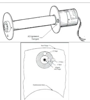
Figure 3-1. Thermopile assembly used in an Eppley Laboratory, Inc., model precision spectral

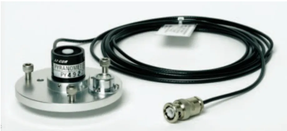
pyranometer (PSP) ... 21 Figure 3-2. (Left) Typical photodiode detector and (right) spectral response of LI-COR pyranometers

LI200SA. Photographs used by permission of LI-COR Biosciences, Inc. ... 21 Figure 3-3. Schematic of an Eppley Laboratory, Inc., model normal incidence pyrheliometer (NIP) (Bahm

and Nakos 1979). Image from the former U.S. Energy Research and Development

Administration, now DOE ... 22

Figure 3-4. Pyrheliometers mounted on an automatic solar tracker. Photo from NREL ... 22 Figure 3-5. Schematics of pyrheliometer alignment diopter configuration (Micek 1981). Image used by

permission from Leonard Micek ... 23

Figure 3-6. Multiple electrically self-calibrating absolute cavity radiometers mounted on solar trackers with control and data acquisition electronics. Photo from NREL ... 24 Figure 3-7. The World Standard Group of six absolute cavity radiometers is used to define the WRR or

DNI measurement standard. Photo from NREL ... 24 Figure 3-8. Schematic of the Eppley Laboratory, Inc., model AHF absolute cavity pyrheliometer. Image

modeled from Reda (1996) ... 25

Figure 3-9. Schematic of the Eppley Laboratory, Inc., model PSP. Image from NREL ... 26 Figure 3-10. Kipp & Zonen model CM22 pyranometers installed in CV2 ventilators. Photo from NREL 26 Figure 3-11. LI-COR model LI-200SA pyranometer with photodiode detector and acrylic diffuser fore

optic. Photo from LI-COR ... 27 Figure 3-12. Four commercially available RSIs: (clockwise from upper left) An Irradiance, Inc., model

RSR2; a Reichert GmbH RSP 4G (previously used by SM-AG); a Yankee Environmental Systems, Inc., model SDR-1; and a CSP-Services GmbH Twin-RSI. Photos by (clockwise

from top) Irradiance, Inc.; Reichert GmbH RSP 4G; NREL; and CSP-Services ... 33

Figure 3-13. Burst (sweep) with sensor signal and the derived GHI, shoulder values, and the DHI. Image

from Wilbert (2014) ... 34

Figure 3-14. RSI calibration station at Plataforma Solar de Almería. Photo by Stefan Wilbert, DLR ... 38 Figure 3-15. Maximum, mean, and minimum RMS deviations of irradiance values with a time resolution

(17)

values as well as for four different corrections were analyzed. Image from Geuder et al.

(2011) ... 39

Figure 3-16. Delta-T Devices, Ltd., SPN1 ... 40 Figure 3-17. Calibration histories for two pyrheliometer control instruments spanning 12 years. Image

from NREL ... 42

Figure 3-18. Pyrheliometer calibration results summarizing (left) Rs compared to SZA and (right)

compard to local standard time. Image from NREL ... 43 Figure 3-19. Pyranometer calibration results summarizing Rs compared to (left) SZA and (right) local

standard time. Image from Daryl Myers, NREL... 48 Figure3-20. Calibration traceability and accumulation of measurement uncertainty for pyrheliometers and

pyranometers (coverage factor k = 2). Image from NREL ... 49 Figure 3-21. Example of SERI quality-control data quality-assurance reporting. Image from NREL ... 60 Figure 3-22. Information flow of a quality-assurance cycle. Image from NREL ... 61 Figure 4-1. The location of the current geostationary satellites that provide coverage around the globe.

Image from NOAA ... 65

Figure 5-1. SOLDAY and SOLMET measurement stations (26 each). Image from NREL ... 88 Figure 5-2. Original 239 stations in the 1961–1990 NSRDB released in 1992 (NSRDB 1992 and 1995)

and the 1,454 stations in the 1991–2005 NSRDB released in 2007. Image from NREL ... 92 Figure 5-3. WRDC measurement stations. Image from NREL ... 96 Figure 5-4. Western Energy Supply and Transmission Associates Solar Monitoring Network of 52

measurement stations (1976–1980). Image from NREL ... 97 Figure 5-5. Pacific Northwest Solar Radiation Data Network operated by the University of Oregon. Image

from NREL ... 98

Figure 5-6. NOAA Solar Monitoring Network of 39 stations (1977–1980). Image from NREL ... 100 Figure 5-7. The Solar Energy and Meteorological Research Training Sites program provided the first

1-minute measurements of multiple solar resource parameters for the United States. Image

from NREL ... 101

Figure 5-8. NREL’s main campus and the Solar Radiation Research Laboratory on South Table

Mountain. Photo from NREL ... 103 Figure 5-9. Historically Black Colleges and Universities Solar Monitoring Network (1985–1996). Image

from NREL ... 110

Figure 5-10. Example data quality summary for one of the 1,454 stations in the 1991–2010 NSRDB update. Image from Steve Wilcox, NREL ... 114 Figure 5-11. Annual mean daily total DNI distribution based on NSRDB/SUNY model results for 1998–

2005 and the corresponding differences between the model and TMY3. (Red circles indicate DNI values from TMY3 < NSRDB/SUNY and blue circles indicate TMY3 >

NSRDB/SUNYA.) Image from Ray George, NREL ... 116 Figure 5-12. TMY3 stations. Image from NREL ... 118 Figure 5-13. BSRN. Image from NREL ... 122 Figure 5-14. The SURFRAD network is operated by the Global Monitoring Division, Earth Systems

Research Laboratory, NOAA. Image from NREL ... 123 Figure 5-15. DOE has operated the 23 Atmospheric Radiation Measurement stations in the southern Great Plains since 1997. Image from DOE ... 127 Figure 6-1. The four stages of a solar power plant project ... 134 Figure 6-2. Geographic information system analysis for available site selection using DNI resource, land

use, and 3% terrain slope. Image from NREL ... 138 Figure 6-3. Geographic information sytsem analysis for available site selection using DNI resource, land

use, and 1% terrain slope. Image from NREL ... 138 Figure 6-4. Yearly sum of DNI as calculated from five modeled data sets: METEONORM, PVGIS,

(18)

Figure 6-5. Resulting uncertainty when combining a base data set of 2%, 4%, 6%, or 8% overall

uncertainty with an additional data set of varying quality. Figure from Meyer et al. (2008)144 Figure 6-6. Upper left: Cumulative frequency distribution for training time of overlapping ground data

and satellite time series. The arrow illustrates the difference between the two curves. Upper right: Corrected satellite cumulative frequency distribution for test period. Lower left: Mapping of original satellite irradiance values to original cumulative frequency distribution (arrow and bottom right image). The original cumulative frequency distribution is first mapped to produce a corrected cumulative frequency distribution, then the corrected cumulative frequency distribution is adjusted to satellite values. Green: ground data from training set; magenta: satellite data from training set; purple: satellite data from test set; yellow: corrected satellite data. Figure from Schumann et al. (2009) ... 145 Figure 6-7. Number of years to stabilize DNI and GHI in (clockwise from upper left) Burns, Oregon;

Eugene, Oregon; Hermiston, Oregon; and Golden, Colorado. Image modified from

Gueymard and Wilcox 2009 ... 148

Figure 6-8. NSRDB/SUNY 10-km grid cells near Harper Lake, California. The upper values shown in text boxes are averaged from (uncorrected) hourly files. The lower values are averaged DNI from corrected maps. The values in red show uncorrected time series mean values, which are substantially lower than the corrected map values. Image from NREL ... 149 Figure 6-9. Monthly mean DNI for Harper Lake (Cell C2) and Daggett TMY3. Minimum and maximum

values for cell C2 are also shown for each month. Image from NREL... 150 Figure 6-10. Desert Rock annual average GHI and DNI from satellite and measurements. Mean bias error

is defined as (satellite - measured)/measured by 100%. Image from NREL ... 152 Figure 6-11. Interannual DNI variability (COV as percent) for 1998–2005. Image from NREL ... 153 Figure 6-12. A 3-by-3 grid layout with anchor cell in the center and 8 surrounding neighbor cells. Image

from NREL ... 154

Figure 6-13. DNI spatial coefficient of variability for a (top) 3-by-3 cell matrix and (bottom) 5-by-5 cell matrix for the average DNI from 1998–2005. Image from NREL ... 155 Figure 6-14. The distribution of the pixels in each spatial variability analysis. The black center pixels

were compared to each of the gray pixels. Images from NREL ... 156 Figure 6-15. Map showing spatial variability among neighboring pixels. Images from NREL ... 156 Figure 6-16. Monthly standard deviation distributions in kWh/m2_{/day for the NSRDB gridded DNI and}

GHI data sets. Illustrations from NREL ... 157 Figure 7-1. Illustration of different forecasting methods for different spatial and temporal scales: TS =

time-series modeling; CM-SI = cloud motion forecast based on sky-imagers; CM-sat = cloud motion forecast based on satellite images; and NWP ... 168 Figure 7-2. Cloud information from sky imagers: (upper left) original images; (middle left) pixel

intensities; (middle right) red-blue ratio, corrected with a clear-sky library; (upper right) cloud decision map; and (bottom) shadow map with irradiance measurements. Sky image and irradiance measurements taken in Jülich, Germany, on April 9, 2013 at 12:59_00UTC in the framework of the HOPE campaign (Macke et al. 2014). Images from the University of

Oldenburg ... 170

Figure 7-3. Example of an optical-flow field. Sky image taken in Jülich, Germany, on April 19, 2013 at 15:30 UTC in the framework of the HOPE campaign (Macke and HOPE-Team forthcoming 2014], Madhavan, Kalisch, and Macke 2014). Image from the University of Oldenburg ... 172 Figure 7-4. Example sky imager-based 5-minute-ahead irradiance forecasts. Location: Universtity of

California at San Diego, November 14, 2012. Image from University of California at San

Diego Center for Energy Research ... 173

Figure 7-5. Schematic overview for detection of cloud motion in satellite images. Images reproduced

from Kuehnert et al. 2013 ... 175

Figure 7-6. Overview of the application of statistical methods and post-processing ... 179 Figure 7-7. Evaluation sites in Germany ... 183

(19)

Figure 7-8. Scatterplots of predicted and measured GHI for (top) high-resolution SKA and (bottom) IFS forecasts. The original forecasts are shown in red, the forecast processed with the linear regression of GHI is shown in blue, and the regression equation is visualized in green. The data are from Dresden, Germany, March 1, 2013–February 28, 2014. ... 187 Figure 7-9. (Solid lines with dots) RMSE and (dashed lines) bias of (red) SKAav and (blue) IFS GHI

forecasts through the time of the day. The data are from 18 German Meteorological Service sites, March 1, 2013–February 28, 2014. ... 188 Figure 7-10. (Solid lines with dots) RMSE and (dashed lines) bias of (red) SKAav and (blue) IFS kt*

forecasts through the (right) time of the day and (left) cosine of the SZA cosΘZ. The data are from 18 German Meteorological Service sites, March 1, 2013–February 28, 2014. ... 188 Figure 7-11. Scatterplot of predicted over measured kt* for (top) high-resolution SKA and (bottom) IFS

forecasts. The original forecasts are shown in red, the forecast processed with the linear regression of kt* is shown in blue, and the regression equation is visualized in green. The data are from Dresden, Germany, March 1, 2013–February 28, 2014; cos(ΘZ) > 0.1 for kt*evaluation, cos(ΘZ) > 0.0 for GHI RMSE and bias. ... 189 Figure 7-12. Probability density function of the clear-sky index derived from (gray) measurements, (red)

high-resolution SKA forecasts, and (blue) IFS forecasts. The data are from 18 German Meteorological Service sites, March 1, 2013–February 28, 2014; cos(ΘZ) > 0.1. ... 192 Figure 7-13. Example days comparing measurements to SKA forecasts with different spatial and temporal averaging—(red) SKA: nearest grid point with hourly resolution; (light blue) SKAav: 5-hour moving average of clear-sky index of the average throughout 20-by-20 grid points. (Left) Clear-sky; data from Lindenberg, Germany, June 19, 2013; and (right) variable cloud

conditions; data from Lindenberg, Germany, March 23, 2013. ... 193 Figure 7-14. RMSE in dependence of the standard deviation of kt*meas (throughout 5 hours) for (left) SKA

forecasts with the application of linear regression ([red] SKA: nearest grid point, [orange] LR: linear regression for GHI, and [yellow] LR-kt* for linear regression for kt*) and (right) with different spatial and temporal averaging ([red] SKA: nearest grid point, [dark blue] SKA20x20 averaged throughout 20-by-20 grid points, [light blue] SKAav 5-hour gliding mean of clear-sky index of the average throughout 20-by-20 grid points, and [green] SKAav, LR.kt*: linear regression of kt*_{applied to SKA}

AV). The data is from 18 German Meteorological Service sites, April 3, 2013–February 28, 2014; training set: last 30 days, all sites. ... 194 Figure 7-15. (Left) Bias of IFS and (right) averaged SKAav forecasts in dependence of the cosine of the

SZA and the predicted clear-sky index kt*. The data are from 18 German Meteorological Service sites, March 3, 2013–February 28, 2014. ... 195 Figure 7-16. (Left) RMSE of IFS and (right) averaged SKA forecasts in dependence of the cosine of the

SZA and the predicted clear-sky index kt*. The data are from 18 German Meteorological Service sites, March 3, 2013–February 28, 2014. ... 196 Figure 7-17. RMSE of IFS and SKA GHI forecasts with different post-processing approaches for (left)

single site forecasts and (right) regional forecasts, derived as mean value of all sites. The data are from 18 German Meteorological Service sites, April 3, 2013–February 28, 2014; training set: last 30 days, all sites. ... 197

(20)

List of Tables

Table 2-1. Radiometric Terminology and Units ... 4

Table 3-1. Solar Radiation Instrumentation ... 20

Table 3-2. WMO Characteristics of Operational Pyrheliometers for Measuring DNIa_{... 28}

Table 3-3. WMO Characteristics of Operational Pyranometers for Measuring GHI or DHI ... 29

Table 3-4. ISO 9060 Specifications Summary for Pyrheliometers Used To Measure DNI ... 30

Table 3-5. ISO 9060 Specifications Summary for Pyranometers Used To Measure GHI and DHI ... 31

Table 3-6. Estimated Pyrheliometer Calibration Uncertainties in Rsi ... 44

Table 3-7. Example of Estimated Direct-Normal Subhourly Measurement Uncertainties (%) ... 45

Table 4-1. Regression Analysis of NASA SSE Compared to BSRN Bias and RMS Error for Monthly Averaged Values from July 1983 through June 2006 ... 69

Table 4-2. HelioClim Compared to Ground Bias and RMS Error for Monthly Averaged Values from 1994 through 1997 ... 70

Table 4-3. Summary of Data Used in MACC-RAD ... 71

Table 4-4. Summary of Applications and Validation Results of Satellite Models— Empirical/Statistical Models (Renné et al. 1999) ... 77

Table 4-5. Summary of Applications and Validation Results of Satellite Models— Empirical/Physical Models (Renné et al. 1999) ... 78

Table 4-6. Summary of Applications and Validation Results of Satellite Models— Broadband Theoretical Models (Renné et al. 1999) ... 79

Table 4-7. Summary of Applications and Validation Results of Satellite Models— Spectral Theoretical Models (Renné et al. 1999) ... 81

Table 5-1. Weighting Factors Applied to Cumulative Distributions ... 89

Table 5-2. Comparisons of TMY2 Data to 30 Years of NSRDB Data ... 94

Table 5-4. NSRDB Data Access Options ... 115

Table 5-5. Ranges of Mean Station Differences for Hourly DNI ... 117

Table 5-6. Bias Differences (Test Data Minus Original 1961–1990 TMY) ... 117

Table 5-7. Standard Deviations of Hourly Data... 117

Table 5-8. Sample MBE and RSME Results for Eight BSRN Stations ... 120

Table 5-9. SolarGIS Validation Summary ... 131

Table 6-1. Site Evaluations ... 135

Table 6-2. Data Sources for DNI Estimation ... 136

Table 6-3. Annual Mean Values of Global and Direct Radiation for Measured and Modeled Data at Desert Rock, Nevada ... 150

(21)

1 Why Solar Resource Data Are Important to Solar

Power

Sunlight is the fuel for all solar energy generation technologies. Like any generation source, knowledge of the quality and future reliability of the fuel is essential to accurate analyses of system performance and the financial viability of a project. With solar energy systems, the variability of the supply of sunlight probably represents the single greatest uncertainty in a solar power plant’s predicted performance. Solar resource data and modeling factor into three

elements of a solar project’s life: • Site selection

• Predicted annual power plant output

• Temporal performance and operating strategy.

The first two items are interrelated. Site selection includes numerous factors, but a top priority is a good solar resource. For site selection, data from individual years and a representative annual solar resource are required to make comparisons to alternative sites and estimate power plant output. Because site selection is always based on historical solar resource data, and because changes in weather patterns occur from year to year, more years of data are better for

determining a representative annual data set. Deriving a typical meteorological year (TMY) is described in Chapter 5. TMY data are used to compare the relative solar resource at alternative sites and to estimate the probable annual performance of a proposed solar power plant. Data from individual years are required to assess the annual variability that can be expected for a proposed location.

In the absence of long-term ground data, development of TMY data for large regions requires the use of models that rely mostly on satellite imagery. In regional terms, identifying prime solar resource areas is fairly simple. The southwestern United States, for example, has broad areas of excellent solar resource. However, narrowing down the data to a specific few square kilometers of land requires considering local impacts; although satellite data are very useful in mapping large regions, individual sites should be vetted by using ground-monitoring stations. Local measurements can be compared to same-day satellite data to test for bias in the satellite model results. Any correction in the satellite model can then be applied to the historical data sets. Correcting any bias in the satellite data will allow the modeler to more accurately apply multiple years of satellite data to generate an improved TMY data set for a site.

After a plant is built, resource data are immediately required to complete acceptance testing. The owner and financiers will insist on verifying that the power plant output meets its design

specifications for a specific solar input. Often the acceptance tests will be for a short duration, perhaps a few days, but the owners will want to extrapolate the results to estimate annual performance. Annual performance estimates can be improved by comparing locally measured ground data to the satellite-derived data for the same time interval.

Accurate resource data will remain essential to a power plant’s efficient operation throughout its service life. Comparison of plant output as a function of solar radiation resource is one global

(22)

indicator of power plant performance. A drop in overall efficiency implies a degradation of one or more power plant components and indicates that maintenance is required.

Last, the realm of resource forecasting is becoming more important for plant dispatch as higher penetrations of solar power are planned for the electric grid. An accurate forecast can increase power plant profits by optimizing energy dispatch into the time periods of greatest value. Although not explicitly covered in this handbook, forecasting requires the same principles described here for historical resource assessment: proper use of satellite- and ground-based data sources and models.

(23)

2 Overview of Solar Radiation Resource Concepts

2.1 Introduction

Describing the relevant concepts and applying a consistent terminology are important to the usefulness of any handbook. This chapter uses a standard palette of terms to provide an overview of the key characteristics of solar radiation, the fuel source for solar technologies.

Beginning with the sun as the source, we present an overview of the effects of the Earth’s orbit and atmosphere on the types and amounts of solar radiation available for energy conversion. An introduction to the concepts of measuring and modeling solar radiation is intended to prepare the reader for the more in-depth treatment in Chapter 3 and Chapter 4. The overview concludes with an important discussion of the estimated uncertainties associated with solar resource data based on measurements and modeling methods used to produce the data.

2.2 Properties of ETR

Any object with a temperature above absolute zero emits radiation. With an effective

temperature of approximately 6,000 K, the sun emits radiation over a wide range of wavelengths, the solar spectral power distribution, or solar spectrum, commonly labeled from high-energy shorter wavelengths to lower energy longer wavelengths as gamma ray, x-ray, ultraviolet, visible, infrared, and radio waves. These are called spectral regions (Figure 2-1). Most (97%) solar radiation is in the wavelength range of 290 nm to 3,000 nm. Future references to broadband solar radiation refer to this spectral range.

Various different extraterrestrial spectral power distributions were derived based on ground measurements, extraterrestrial measurements, and physical models. Some of these spectra deviate strongly from currently accepted standard extraterrestrial spectra as presented in the American Society for Testing and Materials (ASTM) Standard E490 (2006).

Figure 2.1 shows the terrestrial and extraterrestrial spectrum of direct normal irradiance (DNI). Standardized terrestrial spectra for DNI and global hemispherical irradiance on a 37-degree south-facing tilted irradiance are presented in ASTM G173-03 (2006).

(24)

Figure 2-1. The atmosphere affects the amount and distribution of solar radiation reaching the ground. Image from NREL

Before continuing our discussion of solar radiation, it is important to understand a few basic radiometric terms. Radiant energy, flux, power, and other concepts used in this handbook are summarized in Table 2-1.

Table 2-1. Radiometric Terminology and Units

Quantity Symbol SI Unit Abbreviation Description

Radiant

energy Q joule J Energy

Radiant

flux Φ watt W Radiant energy per unit of time

Radiant

intensity I watt per steradian W/sr Power per unit of solar angle Radiant

emittance M watt per square meter W/m2 Power emitted from a surface Radiance L watt per steradian

per square meter W/sr/m2 Power per unit solid angle per unit of projected source Irradiance E, I watt per square

meter W/m2 Power incident on a surface

Spectral

irradiance Eλ watt per square meter per nanometer W/m

2_/nm _{Power incident on a surface} per wavelength

The total radiant power from the sun is remarkably constant. In fact, the solar output (radiant emittance) has commonly been called the solar constant, but the currently accepted term is total solar irradiance (TSI), to account for the actual variability with time. There are cycles in the number of sunspots (cooler, dark areas on the sun) and general solar activity of approximately 11 years. Figure 2-2 shows a composite of space-based measurements of the TSI, normalized to 1

(25)

astronomical unit (AU), the average Earth-sun distance, since 1975, encompassing the last three 11-year sunspot cycles (De Toma et al. 2004).

Figure 2-2. Three solar cycles show the variations of TSI in composite measurements from satellite-based radiometers (color coded) and model results produced by the World Radiation Center (WRC).1_{Image used by permission of the Physical Meteorological Observatory in Davos,}

Switzerland

The measured variation in TSI resulting from the sunspot cycle is ± 0.2%, only twice the

precision (repeatability, not total absolute accuracy, which is approximately ± 0.5%) of the most accurate radiometers measuring the irradiance in space. There is, however, some large variability in a few spectral regions, especially the ultraviolet (wavelengths less than 400 nm), caused by solar activity.

The amount of radiation exchanged between two objects is affected by their separation distance. The Earth’s elliptical orbit (eccentricity 0.0167) brings us closest to the sun in January and farthest from the sun in July. This annual variation results in variation of the Earth’s solar irradiance of ± 3%. The average Earth-sun distance is 149,598,106 km (92,955,953 miles), or 1 AU. Figure 2-3 shows the Earth’s orbit in relation to the northern hemisphere’s seasons, caused by the average 23.5-degree tilt of the Earth’s rotational axis with respect to the plane of the orbit. The solar irradiance available at the top of atmosphere (TOA) is called the extraterrestrial

radiation (ETR). ETR (see Equation 2-1) is the power per unit area, or flux density in watts per

square meter (W/m2), radiated from the sun and available at the TOA. ETR varies with the

Earth-sun distance (r) and annual mean distance (r0):

ETR TSI (r0/r)2 (2-1)

(26)

Figure 2-3. Schematic of the Earth’s orbit. Image from Wikipedia

As measured by multiple satellites (with individual corrections and adjustments applied) throughout the past 30 years, the TSI is 1,366.1 ± 7 W/m2_{at 1 AU. According to astronomical} computations, such as those made by NREL’s solar position software, the variation in the

Earth-sun distance causes the ETR to vary from approximately 1,415 W/m2_{around January 3 to}

approximately 1,321 W/m2_{around July 4.}

From the top of the atmosphere, the sun appears as a very bright disk with an approximate angular diameter of 0.5 degrees (the actual diameter varies by a small amount as the Earth-sun distance varies) surrounded by a completely black sky (apart from the light coming from stars and planets). This angle can be determined from the distance between the Earth and the sun and the sun’s visible diameter. A point at the top of the Earth’s atmosphere intercepts a cone of light from the hemisphere of the sun facing the Earth with a total angle of 0.5 degrees at the apex and a divergence angle from the center of the disk of 0.266 degree (half the apex angle, yearly average). Because the divergence angle is very small, the rays of light from the sun are nearly parallel; these are called the solar beam. In the following, we will discuss the interaction of the solar beam with the terrestrial atmosphere.

2.3 Solar Radiation and the Earth’s Atmosphere

The Earth’s atmosphere is a continuously variable filter for the solar ETR as it reaches the surface. Figure 2-4 illustrates the “typical” absorption of solar radiation by ozone, oxygen, water vapor, and carbon dioxide. The amount of atmosphere the solar photons must traverse, also called the atmospheric path length or air mass (AM), depends on the relative position of the observer with respect to the sun’s position in the sky (Figure 2-4). By convention, air mass one (AM1) is defined as the amount of atmospheric path length observed when the sun is directly overhead from a location at sea level. AM is geometrically related to the solar zenith angle (SZA) as AM = secant of SZA, or 1/Cos(SZA). Because SZA is the complement of the solar elevation angle, AM is also equal to 1/Sin (solar elevation angle). Air mass two (AM2) occurs when the SZA is 60 degrees, and it has twice the path length of AM1. Weather systems,

(27)

the surface or to a solar collector. The cloudless atmosphere also contains gaseous molecules, dust, aerosols, particulates, etc., which reduce the ETR as it moves through the atmosphere. This reduction is caused by absorption (capturing the radiation) and scattering (essentially a complex sort of reflection).

Figure 2-4. Scattering of the direct-beam photons from the sun by the atmosphere produces diffuse radiation that varies with AM (Marion, Riordan, and Renné 1992). Image from NREL

Absorption converts part of the incoming solar radiation to heat and raises the temperature of the absorber. The longer the path length through the atmosphere, the more radiation is absorbed and scattered. Scattering redistributes the radiation in the hemisphere of the sky dome above the observer, including reflecting part of the radiation back into space. The probability of

scattering—and hence of geometric and spatial redistribution of the solar radiation—increases as the path (AM) from the TOA to the ground increases.

Part of the radiation that reaches the Earth’s surface will be reflected back into the atmosphere. The actual geometry and flux density of the reflected and scattered radiation depend on the reflectivity and physical properties of the ground and constituents in the atmosphere, especially clouds.

Based on these interactions among the radiation and the atmosphere, the terrestrial solar radiation is divided into two components: direct beam radiation refers to solar photons that reach the surface without being scattered or absorbed; diffuse radiation refers to such photons that reach the observer after one or more interactions with the atmosphere. These definitions and their usage for solar energy will be discussed in detail in the following section on DNI.

Research into the properties of atmospheric constituents, ways to estimate them, and their influence on the magnitude of solar radiation in the atmosphere at various levels and at the

(28)

2.3.1 Relative Motions of the Earth and Sun

The amount of solar radiation available at the TOA is a function of the TSI and the Earth-sun distance at the time of interest. The slightly elliptical orbit of the Earth around the sun was briefly described above and shown in Figure 2-3. The Earth rotates around an axis through the geographical north and south poles, inclined at an average angle of approximately 23.5 degrees to the plane of the Earth’s orbit. The resulting yearly variation in the solar input results in the climate and weather at each location. The axial tilt of the Earth’s rotation also results in daily variations in the solar geometry throughout the course of a year.

In the northern hemisphere, at latitudes above the Tropic of Cancer (23.5° N) near midday, the sun is low on the horizon during the winter and high in the sky during the summer. Summer days are longer as the sun rises north of east and sets north of west. Winter days are shorter as the sun rises south of east and sets south of west. Similar transitions take place in the southern

hemisphere. All these changes result in changing geometry of the solar position in the sky with respect to a specific location. (See Figure 2-5 generated for Denver, Colorado, by a program available from the University of Oregon2_{.) These variations are significant and are accounted for} in analyzing and modeling solar radiation components using solar position calculations such as

NREL’s Solar Position Algorithm.3

2.4 Solar Resources: The Solar Components

Radiation can be transmitted, absorbed, or scattered by an intervening medium in varying amounts depending on the wavelength (see Figure 2-1). Complex interactions of the Earth’s atmosphere with solar radiation result in three fundamental broadband components of interest to solar energy conversion technologies:

• DNI—Solar (beam) radiation available (of particular interest to concentrating solar power, or CSP, and concentrating photovoltaic, or CPV, technology)

• Diffuse horizontal irradiance (DHI)—Scattered solar radiation from the sky dome (not

including DNI)

• Global horizontal irradiance (GHI)—Geometric sum of the DNI and DHI (total

hemispheric irradiance).

These basic solar components are reacted to the SZA by the expression

GHI = DNI × Cos (SZA) + DHI (2-2)

These components are shown in Figure 2-6.

2_See_{http://solardat.uoregon.edu/SunChartProgram.html}_. 3_See_{http://www.nrel.gov/midc/spa/}_.

(29)

Figure 2-5. Apparent sun path variations during a year for Denver, Colorado. Image from the

Universitity of Oregon Solar Radiation Monitoring Laboratory

Figure 2-6. Solar radiation components resulting from interactions with the atmosphere. Image by

(30)

2.4.1 DNI and Circumsolar Irradiance

The definition of DNI is the irradiance on a surface perpendicular to the vector from the observer to the center of the sun caused by radiation that did not interact with the atmosphere (WMO 2008). This strict definition is useful for atmospheric physics and radiative transfer models, but it results in a complication for ground observations: It is not possible to measure whether or not a photon was scattered if it reaches the observer from the direction in which the solar disk is seen. Therefore, DNI is interpreted differently in the world of solar energy. Direct solar radiation is understood as the “radiation received from a small solid angle centered on the sun’s disk” (ISO 1990). The size of this “small solid angle” for DNI measurements is recommended to be

5 ∙ 10-_{³ sr (corresponding to and approximate 2.5-degree half angle) (WMO 2008). This}

recommendation is approximately 10 times larger than the radius of the solar disk itself (yearly average 0.266 degree). This is because instruments for DNI measurements (pyrheliometers) have to track or follow the sun throughout its path of motion in the sky, and small tracking errors have to be expected. The large field of view (FOV) of pyrheliometers reduces the effect of such tracking errors.

To understand the definition of DNI and how it is measurement by pyrheliometers in more detail, the role of circumsolar radiation has to be discussed. Because of forward scattering of direct sunlight in the atmosphere, the circumsolar region closely surrounding the solar disk (solar aureole) looks very bright. The radiation coming from this region is called circumsolar radiation. For the typical FOV of modern pyrheliometers (2.5 degrees), circumsolar radiation contributes a variable amount, depending on atmospheric conditions, to the DNI measurement. This

contribution can be quantified if the radiance distribution within the solar disk angle and the circumsolar region and the so-called penumbra function of the pyrheliometer is known. Both of these bits of information will be explained in the following. Such an explanation is of particular interest for concentrating solar technologies (CSP or CPV), because the contribution of

circumsolar radiation to the yield of most concentrating power plants is less than the contribution from the DNI measurement. This effect has to be considered in the performance analysis of concentrating collectors to avoid overestimating the intercepted irradiance.

The first bit of information that is required to determine the effect of circumsolar radiation on the pyrheliometer is the solar and circumsolar radiance distribution. This distribution usually shows good radial symmetry around the center of the sun. Thus, it can be accurately described as a function of the angular distance from the center of the sun. This solar radiance profile, normalized to unity in the center of the sun, is called sunshape. The sunshape not varies with time and sky conditions, and the average sunshape determined for a specific site can also be very different from that of another location.

The solar radiance profile has been of interest for scientists of various specializations already for some centuries. In the middle of the 18th century, Bouguer carried out measurements of the disk radiance profile and found that the radiance decreases with increasing angular distance from the center of the sun (Mueller 1897). Between 1920 and 1955, the Smithsonian Institution measured the circumsolar irradiance coming from an annular region concentrically positioned around the sun under the lead of Dr. C.G. Abbot (Watt 1980).

Measurements of the solar radiance profile including the solar disk and the circumsolar region have been carried out by Lawrence Berkeley National Laboratory (LBNL) (Grether, Nelson, and

(31)

Wahlig 1975). The measurements from LBNL are of special importance for solar energy,

because nearly 180,000 measurements were collected from 11 different sites in the United States between 1976 and 1981 and were later digitally published in the LBNL reduced data base

(Noring, Grether, and Hunt 1991). The instrument had a small circular aperture and measured the radiance coming from nearly point-like regions around and inside the solar disk. Other groups used analog photographic techniques to determine the solar radiance profile (for example, Deepak and Adams [1983] and Sandia National Laboratories [see Watt {1980}]). In the 1990s, charge-coupled device cameras were used by the Paul Scherrer Institute and the German Aerospace Center (DLR) (Schubnell 1992), an approach that was followed later by DLR until the end of the last century (Neumann et al. 1998). Recently, a method based on two commercial instruments (Visidyne’s sun and aureole measurement system, Sytem Advisor Model (SAM), and a CIMEL sun photometer) was presented (Wilbert, Pitz-Paal, and Jaus 2013). Other instruments that measure the circumsolar irradiance are documented in Wilbert, Pitz-Paal, and Jaus (2012); Wilbert, Pitz-Paal, and Jaus (2013); Kalapatapu et al. (2012); and Wilbert (2014). Figure 2-7 shows sunshapes derived from LBNL and the first DLR sunshape measurement system. Averages throughout several measurements are shown. A proposed “standard solar scan” was determined by Rabl and Bendt (1982) as an average from LBNL measurements. The term “standard” should not be misunderstood. Here it refers to an average of many sunshapes that deviate strongly from the so-called “standard solar scan.” “DLR mean” shows an average sunshape derived from DLR’s measurements as presented under this name in (Neumann et al. 2002). The other sunshapes are averages of sunshapes within different intervals of CSRs (circumsolar ratio) from (Neumann et al. 2002). They are named corresponding to the CSR interval that was used for the averaging. The CSR can be used to characterize the sunshape to some extent (Buie and Monger 2001). It is defined as

CSR(adisk, alim) = CSNI(adisk, alim) / (CSNI(adisk, alim) + DNI(adisk)) (2-2) Here, CSNI(adisk, alim) is the circumsolar normal irradiance observed in the circumsolar region between the angular distances adisk and alim from the center of the sun. adisk is the solar disk angle (half angle), and DNI(adisk) is the disk irradiance (the normal irradiance caused by the radiation observed within the angular distance adisk around the sun’s center, independent of whether or not the photons were scattered).

The extent of the circumsolar region cannot be defined in a universally valid way. This is because different pyrheliometers and different concentrating collectors use radiation up to individual angular distances alim from the center of the sun. Hence, alim has to be selected depending on the investigated technology. For example, alim = 3.2° is used for the CSR in the LBNL reduced database (Noring et al. 1991), and ≥ 4° would be necessary to allow the complete description of a pyrheliometer measurement following World Meteorological Organization (WMO) recommendations (see next paragraph on penumbra functions).

For the physically exact interpretation of the CSR, adisk is calculated as a function of time using the visible disk radius and the time dependent distance between the sun and the Earth (Wilbert, Pitz-Paal, and Jaus 2013). Depending on the authors and the measurement systems, other angles

(32)

path around the sun. For the LBNL data, a slightly higher angle than the average solar disk angle is used for all measurements (Watt 1980) to avoid instrumental errors that caused an

overestimation of the radiance close to the solar disk angle.

For CPV applications also, the spectral variation of the CSR has to be considered. Spectral CSR values for different wavelengths deviate strongly from each other and also from the

corresponding broadband CSRs (Evans et al. 1980). Average ratios of broadband CSR to spectral CSR between 0.7 and 1.4 have been found for the visible and near-infrared spectrum with the LBNL instrument (for measurements around noon). The spectral dependence of these average ratios found for low CSR levels is opposite to that for high CSRs. Also, the scatter of these ratios for each of the wavelengths investigated by LBNL was quite high (Evans et al. 1980). Similar ratios were found in an analysis based on sunshapes predicted by the three-dimensional Monte Carlo radiative transfer model MYSTIC (Mayer 2009) that is part of the libRadtran package (Mayer and Kylling 2005) and SMARTS2 (Gueymard 2001) in Wilbert, Pitz-Paal, and Jaus (2013). Further, the broadband CSR and especially the spectral CSR depend on the AM.

Figure 2-7. Different sunshapes from Rabl and Bendt (1982) and Neumann et al. (2002). The average solar disk angle and the recommended FOV of a pyrheliometer (WMO 2008) are shown as

vertical lines. Image from Stefan Wilbert, DLR

The other bit of information to determine the effect of the circumsolar radiation on the DNI measurement is the penumbra function of the pyrheliometer. For pyrheliometers, the geometrical penumbra function evaluated at an angular distance a a from the center of the sun Ppyr(a) is defined as the fraction of parallel rays incident on the pyrheliometers aperture at a that reaches the sensor element. It can be calculated using the distance between the aperture window and the sensor element and their respective sizes (Pastiels 1959). Penumbra functions are defined equivalently to angular acceptance functions for CSP or CPV plants, for example, as used in Rabl and Bendt (1982).