Advanced modulation formats and signal processing for high speed spectrally efficient optical communications

HAL Id: tel-01511425

https://tel.archives-ouvertes.fr/tel-01511425

HAL is a multi-disciplinary open access archive for the deposit and dissemination of sci-entific research documents, whether they are pub-lished or not. The documents may come from teaching and research institutions in France or abroad, or from public or private research centers.

L’archive ouverte pluridisciplinaire HAL, est destinée au dépôt et à la diffusion de documents scientifiques de niveau recherche, publiés ou non, émanant des établissements d’enseignement et de recherche français ou étrangers, des laboratoires publics ou privés.

high speed spectrally efficient optical communications

Rafael Rios Müller

To cite this version:

Rafael Rios Müller. Advanced modulation formats and signal processing for high speed spectrally efficient optical communications. Signal and Image Processing. Institut National des Télécommuni-cations, 2016. English. �NNT : 2016TELE0006�. �tel-01511425�

i Spécialité : Electronique et communications

Ecole doctorale : Informatique, Télécommunications et Electronique de Paris Présentée par

Rafael Rios Müller Pour obtenir le grade de DOCTEUR DE TELECOM SUDPARIS

Soutenue le 20/04/2016

Formats de modulation et traitement du signal avancés pour

les communications optiques très hauts débits à forte efficacité spectrale

Devant le jury composé de : Directeur de thèse

Prof. Badr-Eddine Benkelfat Encadrants

Dr. Jérémie Renaudier Dr. Yann Frignac Rapporteurs

Prof. Magnus Karlsson Prof. Gabriella Bosco Examinateurs

Prof. Abderrahim Ramdane

Prof. Darli Augusto de Arruda Mello Prof. Frédéric Lehmann

iii

Contents

CONTENTS ... III

RESUME ... 1

ABSTRACT ... 3

LIST OF ACRONYMS AND SYMBOLS ... 5

LIST OF ACRONYMS ... 5

LIST OF SYMBOLS ... 8

INTRODUCTION ... 13

CHAPTER 1. DIGITAL COMMUNICATIONS ... 19

1.1. COMMUNICATIONS OVER THE GAUSSIAN CHANNEL ... 20

1.2. MODULATION FORMATS ... 22

1.2.1 Hard and soft decision ... 24

1.2.2 Symbol and bit error probability ... 26

1.2.3 Mutual information ... 27

1.3. CHANNEL CODING ... 32

1.3.1 Low density parity check codes ... 34

1.3.2 Spatially coupled LDPC ... 36

1.3.3 Net coding gain ... 38

1.4. SUMMARY ... 40

CHAPTER 2. COHERENT OPTICAL COMMUNICATIONS ... 43

2.1. SYSTEM OVERVIEW ... 44

2.2. LINEAR MODEL ... 46

2.3. RECEIVER AND SIGNAL PROCESSING ... 49

2.3.1 CD compensation ... 52

iv

2.3.4 Carrier phase estimation ... 57

2.4. GAUSSIAN MODEL FOR PROPAGATION OVER UNCOMPENSATED LINKS .... 61

2.4.1 Nonlinear interference ... 61

2.4.2 Nonlinear compensation ... 64

2.5. SUMMARY ... 66

CHAPTER 3. MODULATION FORMAT OPTIMIZATION ... 67

3.1. 8QAM CONSTELLATIONS FOR LONG-HAUL OPTICAL COMMUNICATIONS .. 70

3.1.1 Circular-8QAM vs. Star-8QAM: Sensitivity and phase estimation 71 3.1.2 8QAM constellations: Sensitivity vs BICM-based FEC overhead 77 3.2. TIME-INTERLEAVED HYBRID MODULATION VS 4D-MODULATION ... 83

3.2.1 Time-interleaved hybrid modulation ... 83

3.2.2 4D-modulation formats ... 85

3.2.3 4D vs. Hybrid using mutual information ... 87

3.2.4 Experimental comparison at 2.5 bit/symbol/pol ... 88

3.2.5 4D-coded PAM4 for short-reach applications ... 93

3.3. SUMMARY ... 97

CHAPTER 4. HIGH SYMBOL RATE SPECTRALLY-EFFICIENT TRANSMISSION 99 4.1. SKEW-TOLERANT BLIND EQUALIZER AND SKEW ESTIMATOR ... 100

4.2. FIRST 400GB/S SINGLE-CARRIER TRANSMISSION OVER SUBMARINE DISTANCES ... 109

4.3. FIRST 1TERABIT/S TRANSMITTER BASED ON SUB-BAND TRANSMITTER . 119 4.3.1 Sub-band single carrier vs super-channel ... 126

4.4. SUMMARY ... 130

CONCLUSIONS ... 133

ACKNOWLEDGEMENTS ... 139

v BIBLIOGRAPHY ... 153 PUBLICATIONS ... 165 AS FIRST AUTHOR ... 165 AS CO-AUTHOR... 166 PATENTS ... 168

1

Résumé

La détection cohérente combinée avec le traitement du signal s’est imposée comme le standard pour les systèmes de communications optiques longue distance à 100 Gb/s (mono-porteuse) et au-delà. Avec l'avènement des convertisseurs numérique-analogique à haute vitesse et haute résolution, la génération de formats de modulation d'ordre supérieur avec filtrage numérique est devenue possible, favorisant l’émergence de transmissions à forte densité spectrale. Par ailleurs, la généralisation des liaisons non gérées en dispersion permet une modélisation analytique du canal optique et favorise l'utilisation d’outils puissants de la théorie de l'information et du traitement du signal.

En s’appuyant sur ces outils, de nouveaux formats de modulation à entrelacement temporel dits hybrides et formats multidimensionnels sont étudiés et mise en œuvre expérimentalement. Leur impact sur les algorithmes de traitement du signal et sur le débit d'information atteignable est analysé en détail.

La conception de transpondeurs de prochaine génération à 400 Gb/s et 1 Tb/s reposant sur des signaux à débit-symbole élevé est également étudiée, dans le but de permettre une réduction du coût par bit à travers de l’augmentation de la capacité émise par transpondeur. L'élaboration d'algorithmes de traitement du signal avancés associées à l’utilisation de composants optoélectroniques à l'état de l'art ont permis la démonstration d’expériences records: d’une part la première transmission mono-porteuse à 400 Gb/s sur une distance transatlantique (pour une efficacité spectrale de 6 b/s/Hz), et d’autre part la première transmission à 1 Tb/s basée sur la synthèse en parallèle de plusieurs sous-bandes spectrales (8 b/s/Hz).

3

Abstract

Coherent detection in combination with digital signal processing is now the de facto standard for long-haul high capacity optical communications systems operating at 100 Gb/s per channel and beyond. With the advent of high-speed high-resolution digital-to-analog converters, generation of high order modulation formats with digital pulse shaping has become possible allowing the increase of system spectral efficiency. Furthermore, the widespread use of transmission links without in-line dispersion compensation enables elegant analytical optical channel modeling which facilitates the use of powerful tools from information theory and digital signal processing.

Relying on these aforementioned tools, the introduction of time-interleaved hybrid modulation formats, multi-dimensional modulation formats, and alternative quadrature amplitude modulation formats is investigated in high-speed optical transmission systems. Their impact on signal processing algorithms and achievable information rate over optical links is studied in detail.

Next, the design of next generation transponders based on high symbol rate signals operating at 400 Gb/s and 1 Tb/s is investigated. These systems are attractive to reduce the cost per bit as more capacity can be integrated in a single transponder. Thanks to the development of advanced signal processing algorithms combined with state-of-the-art opto-electronic components, record high-capacity

4

transmission experiments are demonstrated: the first single carrier 400 Gb/s transmission over transatlantic distance (at 6 b/s/Hz) and the first 1 Tb/s net data rate transmission based on the parallel synthesis of multiple spectral sub-bands (at 8 b/s/Hz).

5

List of acronyms and

symbols

List of acronyms

ADC analog to digital converter ASE amplified spontaneous emission AWGN additive white Gaussian noise BER bit error rate

BICM bit interleaved coded modulation BPS bits per symbol

BPSK binary phase shift keying CD chromatic dispersion CMA constant modulus algorithm CFE carrier frequency estimation CPE carrier phase estimation DAC digital-to-analog converter DBP digital backpropagation DCF dispersion compensation fiber DD Direct detection or decision directed DEMUX demultiplexer

DFB distributed feedback laser DFE decision feedback equalizer DMT discrete multi-tone

6

ECL external cavity laser

EDFA Erbium doped fiber amplifier FEC forward error correction FIR finite impulse response

GMI generalized mutual information GNM Gaussian noise model

HD hard-decision

HI horizontal in-phase HQ horizontal quadrature

IC/NLC intra-channel nonlinear compensation IM intensity modulation

ISI inter-symbol interference

ITU international telecommunication union LSPS loop synchronous polarization scrambler LDPC low density parity check

MAP maximum a posteriori MI mutual information

MIMO multiple-input multiple-output ML maximum likelihood

MUX multiplexer

MZM Mach-Zendher modulator NCG net coding gain

NF noise figure

NLT nonlinear threshold

OFDM frequency division multiplexing OSA optical spectrum analyser OSNR optical signal to noise ratio PAM pulse amplitude modulation PBC polarization beam combiner

7 PBS polarization beam splitter

PDM polarization division multiplexing PMD polarization mode dispersion PMF polarization maintaining fibre PSCF pure silica core fibre

PSK phase shift keying

QAM quadrature amplitude modulation QPSK quaternary phase shift keying

RC raised-cosine

RRC root-raised-cosine RZ return-to-zero

RX receiver

SE spectral efficiency SER symbol error ratio SC spatially-coupled

SD soft-decision

SMF single mode fiber SNR signal to noise ratio

SP set-partioned

SSMF standard single mode fibre

TX transmitter

VI vertical in-phase

VOA variable optical attenuator VQ vertical quadrature

WDM wavelength division multiplexing WSS wavelength selective switch

8

List of symbols

  stochastic gradient descent step

nonlinear noise coefficient using Gaussian approximation

  angular frequency   basis waveforms

Bref reference bandwidth

bi i-th bit of a symbol

c speed of light in the vacuum (c=2.99792·108 _m/s)

dmin minimum Euclidean distance

D dispersion factor

erfc() complementary error function expected value f frequency F noise factor Fourier transform G generator matrix h(t) impulse response

h vector representing finite impulse response filter

H parity-check matrix

9

I(X;Y) mutual information

L link length

M modulation order

N0 noise power spectral-density

Nspan number of spans in the transmission line

Pin power per channel at the input of span

Pch power per channel

Pout power per channel at the output of span

PR power ratio between inphase and quadrature components

Q quadrature component

R symbol rate

S constellation rotational symmetry

t time

TS symbol period

x input

13

Introduction

In the past decades the Internet has evolved from a small network between research institutions to a global infrastructure. Internet applications have also evolved from simple services such as file-sharing and e-mail to network demanding ones such as video streaming, online gaming, machine-to-machine communication, etc. These new applications require ever-growing connection speeds. Furthermore, the number of network endpoints has increased from a few million in the 1990s to billions nowadays [1]. With the rise of the internet of things, the number of connected devices will soon reach tens of billions. To support the exponential growth of internet traffic, core networks with ever-increasing rates are necessary. Nowadays, core networks are based on fiber optic communications and the capacity and reach of these optical transport networks have been continuously increasing in the past decades thanks to several technologies: low-loss fibers, optical amplifiers, wavelength division multiplexing, polarization multiplexing, coherent detection, digital signal processing, advanced modulation formats, etc. Rates of 2.5 Gb/s per channel over transoceanic distances were possible in 1990, but since then rates have evolved achieving 100 Gb/s per channel in 2010. Additionally, the use of dense wavelength division multiplexing enables the transmission of around 100 channels in a single fiber resulting in capacities exceeding 10 Tb/s per fiber.

Nowadays, coherent detection in combination with digital signal processing is the de facto standard for long-haul high capacity optical communications systems operating at 100 Gb/s per channel and beyond. With the advent of speed

high-14

resolution digital-to-analog converters, generation of high order modulation formats with digital pulse shaping has become possible enabling the increase of both the rate per channel as well as the spectral efficiency. Furthermore, the widespread use of transmission links without in-line dispersion compensation allows elegant analytical optical channel modeling which facilitates the use of powerful tools from information theory and digital signal processing. In this thesis, these tools are applied to increase the rate per channel and spectral efficiency of long-haul optical communications systems. Concretely, the concepts investigated in this thesis are attractive for next-generation long-haul transponders operating at 400 Gb/s and 1 Tb/s.

This thesis is organized as follows. In Chapter 1 fundamental notions of digital communications, information theory and channel coding over the linear Gaussian channel are revisited. These notions will be later applied to optimize long-haul optical communications transmission systems. Also, the evolution of error correction codes used in long-haul optical communications systems is described. Finally, a short description of low density parity check (LDPC) codes and a novel class of codes called spatially coupled LDPC codes is provided.

Chapter 2 gives a general description of long-haul high-capacity communication systems. The following system blocks are described: the transmitter capable of arbitrarily modulating the 4-dimensional optical field, the optical channel including transmission effects and optical amplification, and the receiver based on coherent detection, polarization diversity, and digital signal processing. The main algorithms in the receiver signal processing are described in detail. Then, an equivalent channel model is described assuming that both amplifier noise and nonlinear interference can be modeled as additive white Gaussian noise for long-haul highly dispersive links. This greatly simplifies system design since it enables the use of the digital communications and information theory tools described in Chapter 1.

In Chapter 3, I investigate modulation format optimization for long-haul high-capacity communication systems building on the tools, models and algorithms described in Chapter 1 and 2. I focus on constellation optimization, multi-dimensional formats and time-interleaved hybrid formats. The four main contributions in this chapter are: the study of 8-ary quadrature amplitude modulation (QAM) formats, and the impact of constellation choice on carrier recovery algorithms; then, several 8QAM constellations are compared in terms of generalized mutual information that better predicts performance considering practical channel coding implementations; afterwards, two solutions providing 2.5 bits per symbol per polarization, the first one based on 4D-modulation and the second on time-interleaved hybrid modulation, are compared; finally, the use of 4D modulation in intensity modulation and direct

15 detection systems based on 4PAM is investigated. All these topics are complemented by experimental results that demonstrate the concepts investigated.

In Chapter 4, the design of next generation transponders based on high symbol rate signals operating at 400 Gb/s and 1 Tb/s is investigated. These high bitrate signals are attractive to reduce the cost per bit as more capacity can be integrated in a single transponder, however at such high symbol rates signals are less tolerant to several imperfections. To deal with one of these imperfections, namely the skew between sampling channels at the coherent receiver, I propose a modified blind equalizer tolerant to receiver skew even after long-haul transmission. Skew estimation is also investigated. Then, thanks to the development of advanced signal processing algorithms combined with state-of-the-art opto-electronic components, record high-capacity transmission experiments are demonstrated: the first single carrier 400 Gb/s transmission over transatlantic distance (at 6 b/s/Hz) and the first 1 Tb/s net data rate transmission based on the parallel synthesis of multiple spectral sub-bands (at 8 b/s/Hz).

19

Chapter 1. Digital

communications

In this chapter, we review basic concepts of digital communications and channel coding over the linear Gaussian channel. Then, we briefly describe the evolution of error correction codes for long-haul optical communications systems. In Section 1.1, we deal with modulation, the process of converting an input sequence of symbols into a waveform suitable for transmission over a communication channel and demodulation, the corresponding process at the receiver of converting the received waveform in a sequence of received symbols. Additionally, we discuss pulse shaping that guarantees inter-symbol interference-free communication while limiting the bandwidth occupied by the transmitted signal. We also describe a received symbol discrete model that considers additive white Gaussian noise and matched filter receiver. Then, in Section 1.2, we discuss modulation formats choice (symbol alphabet) and bit labeling. We introduce useful tools to compare different modulation formats including: minimum Euclidean distance, symbol error rate, bit error rate, mutual information and generalized mutual information. Finally, in Section 1.3, channel coding basics are introduced with a focus on codes used in long-haul optical communications systems. We also give a short description of low density parity check (LDPC) codes and a novel class of codes called spatially coupled LDPC codes. Most of the concepts of Section 1.1 and Section 1.2 can be found in digital communications textbooks such as [2] or in review papers such as [3]. Then, concepts of Section 1.3 can be found in [4] (evolution of channel coding in general

20

from Shannon up to the present) and in [5], [6] (evolution of channel coding schemes for long-haul optical communications).

1.1. Communications

over

the

Gaussian

channel

The problem of converting an input symbol sequence into waveforms s(t) suitable for transmission can be written as:

_(1.1)

where are the discrete symbols we want to transmit over a channel and are the basis waveforms. One example of a basis waveform is the set of delayed rectangle (gate) functions:

_(1.2)

where is the symbol period and the rectangular function:

_(1.3)

However, the rectangle function occupies infinity bandwidth since the Fourier transform of the rectangle pulse is in the sinc function:

(1.4)

To obtain a band-limited basis waveform, we can simply use the sinc pulse in the time-domain:

Now the maximum frequency of the signal s(t) is

. Since the symbol period

is , the symbol rate R equals 1/ and the maximum signal frequency is R/2. The sinc basis function has also other interesting property: at particular instants the function equals only one of sent symbol since for all k (integer). Therefore, at the receiver side, a simple receiver rule would be sampling the waveform at every instant to recover the sent data symbols in the noise-free scenario.

21 The sinc pulse has one drawback which is its long impulse response: the side lobes have high amplitudes that decrease slowly. However, if we accept a slightly higher spectral occupancy, we can use the raised-cosine pulse family. The frequency response of a raised-cosine pulse is:

(1.5)

where is the roll-off factor ( ) and controls the trade-off between the occupied bandwidth and the amplitude of impulse response side lobes. We can simply obtain the impulse response of the raised-cosine pulse

We then write the sent signal as:

_(1.6)

Then, the signal maximum frequency is

and the signal can be recovered

by sampling s(t) every . However, when the received signal r(t) is corrupted by additive white Gaussian noise (AWGN), the optimum receiver is known as the matched filter receiver. The received noise-corrupted signal can be written as:

_(1.7)

where n(t) is AWGN with power spectral density N(f)=N0/2. Using a matched filter

receiver, the received symbol is:

_(1.8)

where is set of orthonormal waveforms. The discrete-time received sequence contains noise estimates of the transmitted symbols .The orthonormality of ensures there is no intersymbol interference (ISI) and the noise sequence ( ) is a set of independent and identically distributed Gaussian random noise variables with zero mean and variance N0/2. To ensure orthonormality, the following requirement

should be satisfied:

_(1.9) This can be achieved using the root-raised cosine pulse shape defined as

22

(1.10)

which is equivalent to solving:

_(1.11) The root-raised cosine pulse shape occupies the same amount of bandwidth as the raised cosine pulse shape. If baseband transmission is used, is a real number (from a set of constellation points), however in passband transmission can be represented as a complex number and the transmitted signal as:

(1.12)

where f0 is the carrier frequency. The receiver needs now an extra block before

matched filter to perform down-conversion and low-pass filtering. Then the discrete-time transmission model can be synthesized as:

_(1.13)

where is still the transmitted symbol belonging to a finite alphabet (now a complex number), is AWGN with variance N0/2 per dimension (real and imaginary) and is the received noise-corrupted symbol.

1.2. Modulation formats

Assuming this linear Gaussian channel model with pass-band transmission, now we focus on the choice of the alphabet. Fig. 1.1 shows six possible modulation formats: BPSK (binary phase shift keying), QPSK (quadrature phase shift keying), 8QAM (8-ary quadrature amplitude modulation), 16QAM, 32QAM and 64QAM containing 2, 4, 8, 16, 32 and 64 possible states, respectively. Defining M as the number of possible states (constellation order), the number of bits that can be transported per symbol period is simply log2(M): 1, 2, 3, 4, 5 and 6, respectively.

23 Fig. 1.1: Example of candidate modulation formats for transmission over a passband channel.

The choice of modulation formats can be done using several criteria. One of the most common criteria is the minimum Euclidean distance (dmin) defined as the

shortest distance between two symbols in the alphabet. Ideally, we would like to maximize this distance to reduce probability of symbol errors when they are corrupted by noise. Tab. 1.1 shows dmin for the formats depicted in Fig. 1.1, with

symbol average energy normalized to one.

Format dmin BPSK 2 QPSK 1.41 8QAM 0.92 16QAM 0.63 32QAM 0.44 64QAM 0.31

Tab. 1.1: Minimum Euclidean distance (normalized to a constellation with unit average symbol energy)

BPSK QPSK 8QAM

24

For the tested formats, the higher is the constellation order, the lower is the minimum Euclidean distance. Furthermore, since we are mainly interested in binary communications, we must investigate the problem of how to map bits to symbols and vice-versa. Fig. 1.2 shows Gray bit-mappings for three real-valued alphabets (from top to bottom): BPSK, 4PAM (4-level pulse amplitude modulation) and 8PAM. Gray mapping ensures that neighbor symbols have only one bit difference. This is useful for transmission over noisy channels since the most common errors are the ones between neighbors, thus reducing the bit error rate compared to non-Gray bit-mapping. Additionally, these same mappings can be extended to complex-valued constellations. For example, two bits can define the mapping of the real component of the 16QAM constellation (equivalent of 4PAM) and the two remaining bits define the imaginary component. The same logic can be extended to QPSK (two parallel BPSK) and 64QAM (two parallel 8PAM). Note that it is not possible to use Gray mapping in the 8QAM and 32QAM constellations depicted in Fig. 1.1, however bit-to-symbol mappings that try to minimize the number of different bits between neighbors can be found usually using local search algorithms such as the binary switching

algorithm [7].

Fig. 1.2: Bit-to-symbol mapping (Gray) for BPSK, 4PAM and 8PAM.

1.2.1 Hard and soft decision

Now, assuming the discrete channel model defined in Eq. 1.13 and modulation formats as the ones defined in Fig. 1.1, we describe the theory of estimating the transmitted symbol after observing a noise-corrupted version of this symbol. The maximum likelihood (ML) symbol detector is:

_(1.14) -5 -3 7 -7 -1 1 3 5 001 011 100 000 010 110 111 101 -3 -1 1 3 01 00 10 11 -1 1 0 1

25 where x can take M values ( ) for a constellation with M symbols. To simplify notation, we write as , as and so on for the rest of

this thesis. Then, the probability density function of receiving y given x (using Eq.

1.13) is:

(1.15) Then, taking the log, which does not change the maximization, we obtain:

_(1.16) This is also known as the minimum distance detector. So maximum likelihood hard-decision can be done by testing all possible symbols in the alphabet ( _{), and then choosing the one closest to the received signal. To}

reduce complexity, especially in the case of M-QAM formats, we can pre-calculate thresholds exploiting the structure of the alphabet. Afterwards, bits are obtained from symbols using a demapper (symbol-to-bit).

Note that if you have a priori knowledge of the distribution of sent symbols, we can alternatively maximize the probability of x given observation of y:

(1.17) Taking the log

_(1.18) This is known as maximum a posteriori (MAP) detection. Note that MAP and ML detectors give the same result if the sent symbols are equiprobable (p(x) is constant for all values of x). This is typically the case for M-QAM formats, but can be different when using, for example, probabilistic shaping [3].

Alternatively, a receiver may be designed to exploit not only the most probable symbol but also the probabilities of every possible symbol [8]. This is known as soft-decision. Suppose we have a constellation with M symbols [ _],

a soft-decision maximum likelihood decoder would simply output the vector [ ] (calculated from Eq. 1.15 if the channel is Gaussian). Alternatively, if we have a priori knowledge on the distribution of sent symbols, we can perform maximum a posteriori soft-decision and the output vector would be [ ].

26

If the alphabet is binary the output vector has only two values and _{, therefore binary soft-decision decoders usually output the likelihood ratio:}

(1.19)

or the log likelihood ratio to ensure numerical stability:

(1.20)

Additionally, even when the constellation is not binary, bit-wise soft decoding can be performed. This is attractive to reduce decoding complexity and it is widely used in practical receivers. Assuming the constellation has log2(M) bits

(b1,b2,…,blog2(M)). The bit-wise log likelihood ratio can be written as:

_(1.21)

where can take values 1 (if symbol of symbol _{equals 0) or 0 (if symbol}

of symbol _{equals 1).}

1.2.2 Symbol and bit error probability

One of the most common metrics to compare different modulation formats is the symbol (resp. bit) error probability which gives the probability of the decided symbol (resp. bit) being different from the actual sent symbol (resp. bit). Given the constellation and the channel, the symbol error probability can be estimated using Monte Carlo simulation or calculated analytically for some constellations. If we also know the bit-to-symbol mapping, the bit error probability may also be estimated or calculated. Fig. 1.3 shows the Monte Carlo simulation of the bit error rate for the formats depicted in Fig. 1.1 (equiprobable sent symbols), using the Gaussian channel and hard-decision decoding based on maximum likelihood estimation. For BPSK and squared QAM formats, we used Gray bit mapping and for 8QAM and 32QAM the bit mappings proposed in [9], [10] respectively.

We observe that the higher the number of bits per symbol the higher is the required SNR to obtain a given BER, the well known trade-off spectral efficiency vs required SNR. In the optical communications community, due to historical reasons BER is usually converted to another performance metric called Q2_{-factor. This metric}

is related to BER using the following formula and BER and Q2_{-factor are used}

27

(1.22)

Fig. 1.3: Bit error rate for several constellations. Solid lines represent formats with Gray mapping and dashed lines formats without Gray

mapping.

1.2.3 Mutual information

Another important metric when choosing the signal alphabet is the mutual information which quantifies the amount of information shared between two random variables. When these two variables represent the sent signal and the received signal (after transmission over a channel and eventually corrupted by noise), the mutual information gives the maximum amount of information that can be transported over the channel. Assuming two random variables: X representing the signal to be transmitted belonging to a finite set of points, and Y representing the received signal after the channel, the mutual information can be calculated as:

(1.23)

then using Bayes rule

(1.24)

where p(x) is the probability distribution of the sent signal: usually a discrete equiprobable distribution where each point belongs to a M point constellation with probability 1/M for each point. Then p(y) is the probability density function of the received symbol: usually the sent symbol distorted by the channel plus random noise. Finally p(x,y) is the joint probability between sent and received signals and

1.E-5 1.E-4 1.E-3 1.E-2 1.E-1 0 5 10 15 20 25

B

ER

SNR E

/N

[dB]

28

p(y|x) is the probability of observing y given transmission of x. Fig. 1.4 shows a simple schematic of an arbitrary channel defined by the conditional probability p(y|x), the amount of information that can be transported in this channel depends on this conditional probability as well as on the choice and distribution of the input symbols.

Fig. 1.4: General channel.

For a transmission over a Gaussian complex channel (see Fig. 1.5), Y corresponds to the received signal in the complex plane corrupted by noise in the form Y=X+Z, where Z has zero mean Gaussian distribution per dimension (in-phase ZI and quadrature ZQ) with variance N0/2, with N0 (noise power spectral density)

being a function of SNR as SNR=Es/N0, and Es is the average symbol energy

( ).

Fig. 1.5: Gaussian complex channel.

The conditional probability density function for the Gaussian channel is simply:

(1.25) Furthermore, the mutual information can be estimated using Monte Carlo simulation as follows: (1.26)

where the sent signal can take M values [ _{] with probabilities}

[ ]. Additionally, K is the number of symbols in the Monte Carlo simulation, is one random sample from the sent signal distribution. For the Gaussian channel, with being one random sample of the normal distribution with variance N0/2 per dimension. When K is sufficient large, the Monte

Carlo simulation converges to the real mutual information.

𝑍~𝒩 0, 0 2 𝑍 ~𝒩 0, 0 2 𝑍 + 𝑗𝑍 ₌ 1 0 2 0

29 Using the Monte Carlo method, Fig. 1.6 shows the mutual information as a function of the signal-to-noise ratio for the equiprobable QAM formats depicted in Fig. 1.1, also known as constellation constrained capacity. We included the Shannon limit (log2(1+SNR)) which defines the upperbound on mutual information over the

Gaussian channel which can be achieved when the distribution of sent symbols is also Gaussian [11]. We observe that each curve saturates at log2(M) and for low

SNR, there is a negligible penalty compared to the Shannon limit coming from the usage of finite equipropable alphabet.

Fig. 1.6: Mutual information over the Gaussian channel for BPSK, QPSK and 8/16/32/64QAM.

The mutual information can also be calculated after performing hard-decision. Fig. 1.7 shows the schematic of the hard-decision Gaussian channel. After receiving y (corrupted by noise), we select as the symbol from the alphabet that maximizes the probability density function of observing y (maximum likelihood detector). Now we have a new random variable representing the distribution of symbols after decision. We can then calculate the mutual information .

0 1 2 3 4 5 6 7 0 5 10 15 20 25 Infor m at ion bi t pe r sy m bol Es/N0 [dB] BPSK QPSK 8QAM 16QAM 32QAM 64QAM

30

Fig. 1.7: Gaussian channel with hard-decision.

Then in Fig. 1.8, we show both (referred as soft-decision mutual information) and (hard-decision mutual information) for QPSK modulation.

Fig. 1.8: Hard-decision vs. soft-decision for QPSK.

We observe that, performing hard-decision reduces the maximum achievable information rate, therefore systems designed to process hard information (decided symbols or bits) requires more power than systems that can take advantage of the

soft information to achieve the same information rate. A general rule of thumb for

maximizing performance can be expressed as: never make hard decisions, instead deliver to the next stage probabilities of possible decisions [8].

Furthermore, we can calculate the bit-wise mutual information, which is interesting to quantify the achievable information rate of multi-level modulation decoded with bit-wise soft-decision. Bit-wise decoding is attractive to reduce decoder complexity in practical receivers. The bit-wise mutual information is sometimes referred as generalized mutual information (GMI) or even BICM mutual information

𝑍~𝒩 0, 0 2 𝑍 ~𝒩 0, 0 2

𝑍

+ 𝑗𝑍

Soft-decision

Hard-decision

= max

31 (related to bit-interleaved coded modulation schemes). The generalized mutual information is simply:

(1.27)

where for each bit we calculate the shared information between the received signal and the transmitted bit, followed by a sum over all log2(M) bits. Compared to mutual

information, there is a loss of information since the generalized mutual information can be developed as:

_(1.28)

and the mutual information as

_(1.29) And since the following inequalities hold:

_(1.30)

_(1.31)

then it is clear that:

32

Fig. 1.9: Mutual information (MI) vs. generalized mutual information (GMI) for 8QAM and 16QAM.

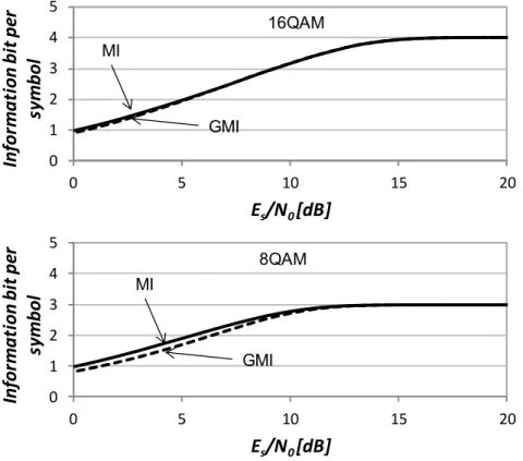
In summary, performing bit-wise soft-decision reduces the mutual information available at the decoder which results in lower achievable information rate. To observe the information rate loss due to bit-wise processing, Fig. 1.9 depicts the comparison between mutual information and generalized mutual information for two formats: 8QAM and 16QAM. We observe that when using 8QAM, there is a higher loss of information compared to 16QAM. This comes from the difference in mapping between the formats. Gray mapping (such as the one of 16QAM) is known to maximize the GMI over the Gaussian channel and there is a small loss coming from bit-wise processing for 16QAM. On the other hand, the bit-wise processing of 8QAM without Gray mapping results in higher penalty coming from the non-Gray mapping.

1.3. Channel coding

The mutual information defines an upper bound on information rate for a given channel using a specific symbol alphabet, however it does not tell us how to achieve this upper bound. This is the goal of channel coding also known as forward error correction (FEC). Channel coding is based on adding redundant information to a bit sequence. At the receiver, after transmission over a noisy channel, the receiver

0 1 2 3 4 5 0 5 10 15 20

Infor

m

at

ion

bi

t

pe

r

sy

m

bol

E

/N

[dB]

Info

rm

at

ion

bi

t

pe

r

sym

bo

l

E

/N

[dB]

33 decoder exploits redundancy to try to recover the sent data. For block codes, we send a codeword of N bits, where K bits represent the data and the remaining N-K bits the redundancy. The amount of redundancy can be quantified by two metrics: the code rate or the overhead. The code rate is defined as:

(1.33)

and the overhead as:

(1.34)

Note that K and N may also represent number of symbols for non-binary codes. For example, the first error correcting code to have achieved widespread use in optical communications systems was the Reed-Solomon code [12] named RS(255,239), with N=255 and K=239 resulting in overhead of 6.7%. These codes used non-binary symbols from an alphabet of length 256 (28_{), therefore after}

conversion to bits we find that each codeword has a total length of 2040 bits. The RS(255,239) code can correct up to 8 symbol errors and was very popular due to its low implementation complexity based on hard-decision decoding.

With the increase of computational power reserved to channel coding, more powerful codes based on longer blocks and product code concatenation gained a lot of attention. The main idea of concatenated product codes [13], [14] is the use of two low complexity component codes and an interleaver to achieve very long codewords which can then be decoded with reasonable complexity. The sequence of data bits is first encoded by a simple component code and then several coded blocks are interleaved before being encoded by another simple component code. The decoding is usually done iteratively, where each component code is decoded alternately and after each iteration performance improves until saturation. Most of the codes defined in ITU G.975.1 (specification of error correction codes for optical communications [15]) are based on concatenated product codes and typical block length is around 500.000 bits with overhead around 7% and hard-decision. One popular implementation is the one defined in Appendix I.9 of G.975.1 where each component code is a BCH code. This code has a pre-FEC BER threshold of 3.8∙10-3 _{to obtain a}

post-FEC BER below 10-15_.

With the advent of coherent detection and high resolution analog-to-digital converters, soft-decision has become attractive to provide even better performance compared to the previously mentioned codes based on hard-decision. For example,

34

low density parity check (LDPC) codes belong to a class of block codes first proposed by Gallager [16] which when paired with soft-decision iterative decoding can provide performance very close to the Shannon limit of the Gaussian channel. One undesired property of LDPC codes is the error floor: the fact that beyond a given SNR, the BER does not drop as rapidly as in the waterfall region. To tackle this problem, soft-decision LPDC are often used as an inner code to reduce the BER to a level usually between 10-3 _{and 10}-5_{, followed by a small overhead hard-decision code}

to further reduce the BER to a level typically below 10-15_{. The use of LDPC with}

overhead around 20% became very popular for ultra-long-haul optical communication systems and it is currently used in commercial products. However, there is still room for improvement and a straightforward way to further increase channel coding performance of block codes is to increase the block size. Unfortunately, a block length beyond 30000 bits becomes very challenging for real-time applications at bitrates beyond 100 Gb/s (typical in long-haul optical communication systems). Nevertheless, a new class of codes referred as spatially coupled (SC-) LDPC can enable virtually arbitrarily long codewords that can be decoded with a simple decoder. Although this class of codes was introduced more than a decade ago, their outstanding properties have only been fully realized a few years ago, when Lentmaier et al. noticed that the estimated decoding performance of a certain class of terminated LDPC convolutional codes with a simple message passing decoder is close to the optimal MAP threshold of the underlying code ensemble [17]. Additionally, these codes have outstanding performance in the error floor region [18]. In this thesis, the outstanding performance of spatially-coupled LDPC codes has been used to obtain extra performance gain in record ultra-long-haul experiments (Chapter 4). In next section, we briefly describe LDPC codes and the spatially-coupled LDPC codes. For a exhaustive description of these codes, please refer to [17], [19], [5].

1.3.1 Low density parity check codes

To introduce low-density parity check codes, we start with a toy example. We use the Hamming code (7,4) which is a short block code as an example [20]. This code is defined by the generator matrix:

_(1.35)

35 To generate the 7-bit long code word x=[x0,x1,x2,x3,x4,x5,x6] from 4 data bits d=[d0,d1,d2,d3] we simply perform matrix multiplication using binary logic:

_(1.36)

This encoder structure defines three parity check equations also based on binary logic:

_(1.37)

_(1.38)

_(1.39)

This set of equations can be synthesized in matrix notation:

_(1.40)

_(1.41)

where H is the parity check matrix. In this particular case, the percentage of “1”s in the matrix is around 62%, however for LDPC codes this percentage is much lower (usually below 1%) so we refer to these parity check matrices as low-density. Additionally, in practical codes the block length is much longer (usually beyond 1000 bits). Nevertheless, this toy example is useful to understand some key concepts of LDPC codes. These codes are usually described by their variable node degree and check node degree. The number of “1”s per row defines the check node degree which in our example is 4. Then, the number of “1”s per column defines the variable node degree which in our example is not constant, so we use instead the variable node degree profile. The degree profile indicates the percentage of nodes of certain degree. The Hamming exemplary code has variable node degree profile: 3/7 of columns have degree 1, 3/7 degree 2 and 1/7 degree 3. Codes with both constant check node degree and constant variable node degree are called regular. On the other hand, codes with non-constant variable node degree and/or non-constant check node degree are called irregular LDPC. The Hamming code example is irregular.

At the receiver, we have a noisy observation of the code word:

36

where n=[n0,n1,…,nN-1]T is a vector of complex zero mean Gaussian independent noise. An optimal maximum a posteriori (MAP) decoder selects the estimated code word that maximizes the probability:

_(1.43) Since we suppose each code word is equiprobable, we can simply maximize the likelihood and obtain the maximum likelihood (ML) estimator:

_(1.44)

For long codewords, MAP and ML estimation are intractable problems, so practical LDPC use sub-optimal decoding with reasonable complexity which exploits the underlying structure of LDPC codes (sparse graph [21]). LDPC decoding is usually based on belief propagation (also known as sum-product algorithm [22], [23]). This algorithm performs exact inference on loop-free graphs (trees) by calculating marginal distribution of unobserved nodes (data in the case of channel coding). However, LDPC codes graph structure is not free of loops (acyclic) so belief propagation does not perform exact inference and it is suboptimal. Belief propagation in graphs with loops is also known as “loopy” belief propagation and iterations are used until the algorithm converges. Nevertheless, the performance penalty of LDPC decoding under belief propagation can be very low and LDPC codes are very popular and are present in several standards.

1.3.2 Spatially coupled LDPC

One goal of spatially-coupled LDPC codes, is to provide very long codewords. This is done simply by connecting neighboring blocks. For example, if we want to couple every block of the Hamming code (7,4) without changing the degree distribution, we could simply rewrite the parity check equations as:

(1.45) (1.46) (1.47) We define the exponent i as the block number, and now for each parity equation we included one variable that depends on the previous block (i-1). So now we decompose the parity check matrix in two sub-matrices:

37 _{(1.48) (1.49)}

And the previous parity check matrix for the uncoupled case is simply . The number of previous blocks connected defines one design parameter referred as syndrome former memory, which here is 1. Here we showed a deterministic connection between blocks, however these constructions are difficult to analyze so random connection has also been proposed [19]. Now the equivalent parity check matrix of the infinitely long spatially coupled code is:

(1.50)

If we now count the number of “1”s and per row and per column, we obtain the same degrees as the underlying code. However, this infinitely long code is not practical and we need to terminate it. There are two options for termination. The first one referred as tail-biting which preserves the check and variable node degree:

(1.51)

The second one is terminated, as follows:

(1.52)

One potential disadvantage of the terminated approach is the fact that it has one extra row compared to the tail-biting method which causes rate loss (higher overhead). However, if we increase the sub-matrix repetition (make the equivalent matrix very large) the rate loss becomes smaller. This small extra overhead can also be attractive since, the extra parity bits are present on the codeword edges. Therefore, the edge bits are more protected than the center bits so when we start the

38

iterative decoding, the first bits to be decoded are the ones in the edge and the information propagates to the central bits (decoding wave). Furthermore, since the decoding happens only close to this wave we can design simple decoders referred here as windowed decoders [24], [25]. The windowed decoder has a window size that defines how many sub-blocks it is decoding. For example, assuming the terminated example, the total parity check equation is written as:

_(1.53)

where _{are the codewords for each block i. Without windowed decoder, decoding}

would be performed over the whole matrix . However, reduced complexity can be achieved by exploiting the sub-matrix repetition structure and the decoding wave behavior (from the edges to the center). Therefore, a windowed decoder would start with decoding some blocks in the edge (number of blocks related to the window size), and then as edge blocks are decoded the window slides toward the matrix center. This technique of terminated SC-LDPC with windowed decoder will be used in Chapters 3 and 4 as a code of choice in transmission experiments.

1.3.3 Net coding gain

To compare different codes in transmission systems, the most useful performance metric is the net coding gain. This metric tells what is the difference (in dB) of required signal to noise ratio (SNR) between coded transmission compared to uncoded transmission while accounting for the extra overhead to achieve a given performance. For example, if we use uncoded QPSK and the target performance BER equals to 10-15_{, we know that the required SNR is 18 dB. Let us assume that we}

have an arbitrary binary code where 50% of the codeword is reserved for redundancy bits (code rate equals to 0.5) and we measure 10 dB as the required SNR to achieve 10-15 _{BER after decoding. Then, the coding gain at 10}-15 _{BERis simply 8 dB (18 dB –}

10 dB). However remember that to transmit the same amount of information with the coded transmission, we need to increase its symbol rate by 100% (3 dB). So accounting for this extra required power to increase the symbol rate, we obtain the net coding gain at 10-15 _{BER of 5 dB (8 dB – 3 dB). In this example, the SNR}

threshold is 10 dB equivalent to a pre-FEC BER of 7∙10-4 _{or Q}2_{-factor threshold of 10}

39 For binary codes, an upper bound of the maximum net coding gain can be calculated as a function of the code rate as follows:

(1.54)

Therefore, we can calculate the net coding gain upper bound for two decoding approaches: hard-decision ( ) and soft-decision ( ). Table 1.2 summarizes required SNR values as well as maximum net coding gains for hard-decision and soft-hard-decision.

r OH Hard-dec. Soft-dec. 0.934 7% 18 dB 7.6 dB 6.5 dB -0.3 dB 10.1 dB 11.2 dB 0.833 20% 18 dB 5.9 dB 4.6 dB -0.79 dB 11.31 dB 12.61 dB 0.8 25% 18 dB 5.4 dB 4.1 dB -0.96 dB 11.64 dB 12.94 dB 0.5 100% 18 dB 1.8 dB 0.2 dB -3 dB 13.2 dB 14.8 dB

Tab. 1.2: Symbol rates with corresponding FEC overheads and Q² thresholds

Fig. 1.10 depicts the net coding gain (NCG) as a function of the overhead for binary codes. Solid and dashed lines represent the maximum net coding gain of an ideal soft-decision (SD) and hard-decision (HD) error correcting codes respectively. We also show NCG of implementations of several codes employed in long-haul optical communications. The first generation based on 7% hard-decision FEC is represented by squares. Empty square represents the first code to achieve widespread use in optical communications due to its very low implementation complexity: RS(255,259) with around 6.2 dB of NCG. Then, with the same overhead, the filled square represents the concatenated hard-decision 7% code in the ITU standard [15] (Appendix I.9). At around 9 dB of NCG, this FEC is present in many commercial products thanks to its high coding gain with reasonable decoding complexity. Subsequently, the next generation of codes exploited the soft information available at coherent receivers and 20% SD-FEC were introduced and are now present in commercial long-haul high performance applications. One example of

40

these new soft-decision codes based on LDPC is represented by a circle [26] with around 11 dB of NCG. There is still room to reduce the gap to the limit and achieve higher NCG by increasing the overhead and/or using more powerful codes such as ones based on spatial coupling. This family of codes has very interesting properties (described in previous paragraphs). For example, 25% SD-FEC based on SC-LDPC [27] has around 1dB advantage over 20% LDPC-based SD-FEC as depicted in the figure (diamond) and it is closer to the SD-NCG limit. Those codes based on spatial coupling are attractive candidates to boost performance of next-generation optical communications systems.

Fig. 1.10: Net coding gain at 10-15 _BER.

1.4. Summary

In this chapter we reviewed basic concepts of digital communications and channel coding and we introduced some tools that will be used in the next chapters: pulse shaping, modulation formats, (generalized) mutual information, FEC overhead, etc. In Chapter 2, we describe the optical communications systems based on coherent detection and we show that its equivalent channel model can be well approximated by the Gaussian channel model, therefore all the tools presented here can be applied to optimize its performance.

In this chapter, we also reviewed the evolution of error correction codes for optical communications. We focused and we briefly described the concept of spatially-coupled LDPC codes. Again, a more detailed description of this class of

5 6 7 8 9 10 11 12 13 14 0 5 10 15 20 25 30 N e t c o di ng g ai n [dB ] FEC overhead [%] 7% HD-FEC (concat. BCH) 20% SD-FEC (LDPC) 25% SD-FEC (SC-LDPC) 7% HD-FEC RS(255,239)

41 codes can be found in [5], [17], [19]. SC-LDPC codes will be used in several experiments described in Chapters 3 and 4.

43

Chapter 2. Coherent optical

communications

This chapter deals with several aspects of long-haul transmission systems based on wavelength division multiplexing and coherent detection. Coherent detection in combination with digital signal processing recently became the de facto standard for long-haul high capacity systems. Not only a coherent receiver has better sensitivity than a quadratic receiver, but also when in combination with high resolution analog-to-digital converters it is capable to reconstruct in the digital domain (with high fidelity) the optical field at the receiver. Hence, this enabled the use of signal processing algorithms to compensate fiber transmission linear impairments and to mitigate nonlinear impairments as well as fully exploit the four dimensions of the optical field (in-phase and quadrature of two orthogonal polarizations). Additionally, the introduction of high resolution high speed digital-to-analog converters at the transmitter gave designers a whole new degree of freedom. Now it is possible to modulate the 4-dimensional optical field with an arbitrary waveform in an optical bandwidth beyond 50 GHz. For example, the transmitted signal can now be shaped using digital filters resulting in increased spectral utilization through Nyquist pulse shaping. We can also use the arbitrary waveform functionality to adapt the modulation format for each transmission scenario using arbitrary constellations resulting in optimized performance. Finally, with the exponential increase of number of transistors in an integrated circuit, we have more and more available computational power to be used in signal processing algorithms and channel coding implementations resulting in several possibilities for performance increase.

44

This chapter is divided into 5 sections. First, Section 2.1 gives a general description of the three main blocks of long-haul high-capacity communication systems: transmitter, channel and receiver. In Section 2.2, we focus on modeling the optical channel in the linear regime. Fiber attenuation, amplifier additive noise, chromatic dispersion and polarization dependent effects are described. Next, in Section 2.3, receiver signal processing algorithms that mitigate linear impairments are detailed. In Section 2.4, we include non-linear effects in the model assuming that non-linear interference can be approximated as excess additive Gaussian noise. Finally, in the last section we summarize the chapter main concepts.

2.1. System overview

Fig. 2.1 shows a typical long-haul optical communication system with optical amplification and wavelength division multiplexing (WDM). In WDM, the light emitted by multiple (Nch) laser sources at different wavelengths (λn) are modulated

independently and simultaneously propagated over the same fiber. Therefore, we have Nch independent transmitters (TX) which can be referred as channels. The signals coming from each transmitter are then combined using a multiplexer (MUX) before transmission. The transmission link is made of Nspan spans of single mode fiber (SMF) separated by optical amplifiers that compensate for span loss. Erbium doped fiber amplifiers [28] (EDFA) operating on the C-band are the most widely used optical amplifiers. A typical C-band EDFA amplifier bandwidth is around 32 nm (centered at 1545 nm), therefore roughly 80 channels can be simultaneously amplified by a single EDFA considering 50 GHz channel spacing. After transmission, channels are separated by a demultiplexer before being detected by Nch coherent receivers.

Fig. 2.1: Three main communication systems components: transmitter, channel and receiver.

To maximize the spectral efficiency, all physical dimensions available must be exploited by each transmitter. The main function of an optical transmitter is to convert an electrical signal into the optical domain. Here, we focus on transmitters that can independently modulate the amplitude and phase of the two optical polarizations of

x Nspan Channel EDFA M U X D EM U X TX λ1 TX λ2 TX λ_Nch

…

…

…

…

Chapter 2 – Coherent optical communications

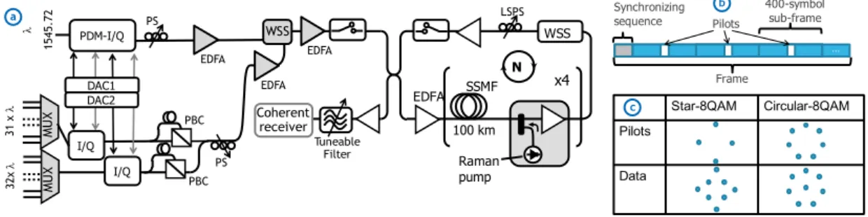
45 the optical field over a large electrical bandwidth. For long-haul applications, this is typically achieved by cascading a laser source with Mach-Zehnder modulators (MZM) and a polarization beam combiner (PBC) as shown in Fig. 2.2.

Fig. 2.2: Transmitter modulated in-phase and quadrature component of two orthogonal polarizations based on Mach-Zehnder modulator (MZM).

The goal of the optical transmitter is to transmit at every instant k, two complex symbols and in the horizontal and vertical polarizations, respectively. The electrical waveforms containing data to be transmitted are generated by four synchronized digital-to-analog converters (DAC). At the output of each DAC, we have 4 electrical waveforms: (2.1) (2.2) (2.3) (2.4)

where hRRC_{(t) is the impulse response of the root-raised cosine filter and R is the} symbol rate. Roll-off factor of RRC filters and the symbol rate define the signal occupied bandwidth. To modulate each polarization, we use external modulators with a nested structure, comprising two MZM in parallel with π/2 shift between their outputs. The light from the laser with central frequency fTX=ωTX/2π is first split in two copies. Each copy is sent into a distinct modulator driven with different electrical data. Finally, a PBC recombines the output of both modulators onto two polarizations

𝐡 . ( . ) DAC DAC 𝐡 . ( . ) DAC DAC 2 2 𝑉 TX TX DSP MZM PBC _{= ( ) ( / )} ∞ = ∞ _{= ( ) ( / )} ∞ = ∞ 𝑉 _{= (} 𝑉_{) ( / )} ∞ = ∞ 𝑣 _{= (} 𝑉_{) ( / )} ∞ = ∞ _{= ( ) ( / )} ∞ = ∞ _{= ( ) ( / )} ∞ = ∞ 𝑉 _{= (} 𝑉_{) ( / )} ∞ = ∞ 𝑣 _{= (} 𝑉_{) ( / )} ∞ = ∞ _{= ( ) ( / )} ∞ = ∞ _{= ( ) ( / )} ∞ = ∞ 𝑉 _{= (} 𝑉_{) ( / )} ∞ = ∞ 𝑣 _{= (} 𝑉_{) ( / )} ∞ = ∞ 𝑉 ∼ 𝒩 0, 𝜎𝐴 2 𝑉 _{∼ 𝒩 0, 𝜎} 𝐴 2 sin 𝜔 + 𝜃 sin 𝜔 + 𝜃

46

of the polarization division multiplexed channel. Then the WDM multiplex, comprising

Nch channels is amplified before being transmitted. The channel spacing choice depends on several parameters: the channel occupied bandwidth, the precision of the central frequency of the signal carrier, etc. We can obtain the information spectral efficiency as the ratio between the bitrate per channel and channel spacing. Typical channel spacing is 50 GHz, but a finer granularity grid of multiples of 12.5 GHz become increasingly popular to provide better flexibility to optimize spectral efficiency.

2.2. Linear model

In this section, the principal transmission linear impairments for long-haul transmissions are briefly described and modeled. Here we discuss fiber attenuation, impact of amplifier noise in signal-to-noise ratio, chromatic dispersion and polarization mode dispersion.

Fiber attenuation is one of the main impairments limiting optical communication systems. When an optical signal propagates through an optical fiber its power is attenuated due to absorption and scattering loss. The power at the output of a fiber span (Pout [dBm]) as a function of the input power (Pin [dBm]) can be simply

written as:

_(2.5)

where L is the span length typically in [km] and α is the fiber attenuation typically in [dB/km]. The attenuation suffered by the propagating signal depends on the wavelength. The C-band (around 1550 nm) is the fiber window where the minimum of attenuation is located. The attenuation value in the C-band is usually around 0.2 dB/km for standard fibers, and can be as low as 0.148 dB/km for enhanced fibers.

To compensate for span loss, long-haul optical systems incorporate periodic optical amplifiers. C-band Erbium doped fiber amplifiers are the most widely used nowadays as they operate in the lowest fiber attenuation window. These amplifiers amplify the weak input signal from the previous span and launch it again into the next span at high power. However, EDFAs also introduce additive noise through amplified spontaneous emission (ASE) which degrades the optical signal-to-noise ratio (OSNR). The OSNR is defined as the ratio between the power of the signal and the power of the noise in a reference bandwidth, i.e. 12.5 GHz. The OSNR degradation can be measured by the amplifier noise factor (F) which is the linear ratio between the linear SNR at the input ( ) and at the output ( ) of the amplifier. The