HAL Id: hal-00768442
https://hal.univ-brest.fr/hal-00768442
Submitted on 23 Dec 2012
HAL is a multi-disciplinary open access
archive for the deposit and dissemination of
sci-entific research documents, whether they are
pub-lished or not. The documents may come from
teaching and research institutions in France or
abroad, or from public or private research centers.
L’archive ouverte pluridisciplinaire HAL, est
destinée au dépôt et à la diffusion de documents
scientifiques de niveau recherche, publiés ou non,
émanant des établissements d’enseignement et de
recherche français ou étrangers, des laboratoires
publics ou privés.
Design under Constraints of Availability and Energy for
Sensor Node in Wireless Sensor Network
Van-Trinh Hoang, Nathalie Julien, Pascal Berruet
To cite this version:
Van-Trinh Hoang, Nathalie Julien, Pascal Berruet. Design under Constraints of Availability and
Energy for Sensor Node in Wireless Sensor Network. IEEE International Conference on Design and
Architectures for Signal and Image Processing (DASIP), October 2012, Oct 2012, Karlsruhe, Germany.
pp.E-ISBN : 978-2-9539987-4-0. �hal-00768442�
Design under Constraints of Availability and Energy for Sensor
Node in Wireless Sensor Network
Van-Trinh HOANG, Nathalie JULIEN, Pascal BERRUET
[email protected], [email protected], [email protected] Lab-STICC/University of South-Brittany, Research Center, BP 92116, 56321 Lorient, France.
Abstract—Wireless Sensor Network (WSN) technology has been getting a lot of attention in recent years due to its low-cost, portability, easy deployment, self-organisation, and reconfigura-bility. Two main challenges faced by designers are availability and power/energy management for WSN. This paper presents a design for a wireless sensor node, which provides automated reconfiguration for both availability and energy-efficient use. This design introduces an original device named Power and Availability Manager (PAM) combined with a FPGA. The first one is considered as the intelligent part for the best use of energy and fault-tolerance, while the other enhances the availability in case of hardware failure for a node. Simulation model of these solutions together is based on General Stochastic Petri Net (GSPN). The results indicate a gain of availability from 9% to 31% for sensor node over twelve years, from 9% to 46% for sensor cluster over eighteen years, from 11% to 45% for whole network over fifty years. Our approach also results in significant energy-saving : up to 61% by using DPM policy, and up to 62.5% by using DPM and DVFS policies over seven days. These results allow us to evaluate and to show a design of WSN node for increased availability as well as energy-saving by using our approach.
Index Terms: availability, energy-efficiency, fault-tolerance, reconfiguration, WSN, PAM device, FPGA.
I. INTRODUCTION
Wireless Sensor Network (WSN) is ideally suited as founda-tion for many applicafounda-tions. Thanks to its portability, it may be carried out on everywhere from the human body to be deeply embedded in the environment. Wireless Sensor node can easily be deployed in large space with dramatically less complexity and cost compared to wired networks. Additionally, sensors can self-organize to form routing paths, collaborate on data processing, and establish hierarchies. The WSN is also re-configurable by easily adding and removing sensor nodes. Thus it is the most favorite candidate for many applications such as area monitoring, environment monitoring, industrial monitoring, etc.
Each WSN consists of small sensors, with limited process-ing and computation capacity, memory, and battery power. Besides, the sensor nodes are deployed in the harsh envi-ronment, thus the human intervention is mostly impossible in case of hardware failure and energy depletion. Therefore, both availability and energy-efficient consumption are the important key features that decide the success of such a WSN. Many works are available on availability such as [4], [10], [9] or on energy-efficiency such as [12], [1], [7], separately. But there are few works that take into account both aspects. Thus our goal is to provide a design of sensor node for increased availability as well as energy-saving. This paper is organized
as follows. In section II, the related work is presented. In section III, we expose problem issues encountered in a sensor node and our approach using PAM and FPGA for available, fault-tolerant and energy-efficient system. The simulation tests are provided in section IV. Section V contains conclusions and future works.
II. RELATED WORKS
A. Availability
Ringwald and Rmer [9] provide a list of possible prob-lems and their causes on WSN during deployment. These problems can be detected by means of passive inspection method [11] that does not require any modification of sensor network. Unfortunately, they do not specify any methods to fix these problems. High dependability of computing systems is paramount requirement for embedded system, but advances in manufacturing the semiconductor device increase the inter-mittent and permanent faults. Constantinescu [4] proposes a method for evaluating availability of fault-tolerant processor by using GSPN modeling [5], but his method needs a double hardware requirement that occupies more system space. Suho-nen [10] presents remote diagnostics and performance analysis that comprise self-diagnostics on embedded sensor nodes, but he does not indicate in detail the reasons of a sensor node failure.
B. Energy-Efficiency
In this domain, two major methods for optimizing energy consumption are Dynamic Power Management (DPM), and Dynamic Voltage and Frequency Scaling (DVFS) [1]. The strategy of first one is to turn off a part of the circuit or run it in degraded mode (sleep or deep sleep mode) which reduces consumption, but it requires a suitable wake-up time and power overhead that do not violate the operation of application. The second one allows decreasing the supply voltage and operating frequency under application permission. Since there are large overheads by using DVFS, thus DPM is more preferable to use in our approach. Hassanein and Luo [12] propose Reliable Energy Aware Routing (REAR) that includes local node selection, path reservation, and path request broadcasting delay to provide a reliable transmission environment to reduce retransmissions caused by unstable paths. Miguel and Juan [7] introduce a novel architecture that takes into account addressing scheme, topology control, multi-hop synchronization, task scheduling, application data model to extend the battery life.
Supervisor Network level Cluster level Node level Sink Relief Sink Gateway Temporary Gateway Candidate Gateway Normal Node
Fig. 1. Architecture of wireless sensor network
C. Objective
In all these attempts, an overall approach that takes into account both availability and energy-efficiency aspects is still missing. Therefore, a novel available and energy-efficient design is proposed for sensor node. As a result, that leads to a more reliable and efficient sensor network. The next section describes in detail our approach.
III. OUR APPROACH
A. Architecture and hardware configuration of WSN
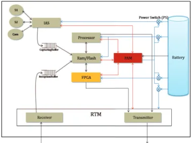
Fig. 2. Hardware configuration of wireless sensor node
As mentioned earlier, the aim of our approach is to provide a design of sensor node that takes into account both availability and energy-efficiency. Since the centralized network has the drawbacks such as limied space coverage and problem of buffer overflow at sink node. Therefore, we focus at decentral-ized network for our approach. According to our vision, the WSN is considered in three levels of hierarchy. The lowest one of which is sensor node level, the medium one is cluster level, and the highest one is network level. Additionally, six types of sensor are considered in our network as indicating in Figure 1.
In above figure, Normal Nodes, Temporary, and
Candi-date Gateway capture and deliver data directly or through
their neighbor nodes to Gateway, which is considered as the head of sensor cluster. Then Gateway aggregates the sent data and transmits it to the Sink through other Gateways. Finally, the Sink sends data to the supervisor for checking. In case
of failure of Gateway, Temporary Gateway replaces tem-porarily it and actives a mechanism to select a new Gateway in the set of Candidate Gateway. The Relief Sink is used to replace immediately the Sink if it is out-of-order, because this problem is the most critical that leads to lose whole network. The Relief Sink is inactive until it receives wake-up message from the Sink. Our hardware configuration model of a node is illustrated in Figure 2 that includes a processor, a RAM/FLASH memory, a Power Availability Manager (PAM), a configurable zone of FPGA, an Interface for Actuator and Sensors (IAS), a Radio Transceiver Module (RTM), and a battery with DC-DC converters.
B. Problem issues and solutions of sensor node
Our self-reconfigurable sensor node can detect wrong be-haviors and failures due to software, hardware or energy when they occur, then take corrective solution to make itself less vulnerable. For automating failure detection, PAM block polls periodically each component of sensor node, as illustrated in Figure 3. In order to detect processor failure, PAM sends a message to it. If PAM does not receive any feedback from processor, it is considered as failed. In case of memory, PAM writes and reads a data on it and then compares this data with the original one. If they are not the same, the memory is failed. For the sensors interface and the radio module, PAM stores the value of energy consumption (capturing, reception, transmission) of each component and supervises the energy consumption when they are operating. If there is a large difference with the same amount of data between the stored energy value and the operating energy value, the sensors or the radio module is considered as failed.
To mitigate the data conflict, two First In First Out (FIFO) buffers are used in which CapturingBuffer stores the captured data, and ReceptionBuffer saves the data sent by other nodes. The Ram memory is also partitioned in three zones for storing capturing data, receiving data and transmitting data. Based on the list of possible issues [9], and our knowledge, several
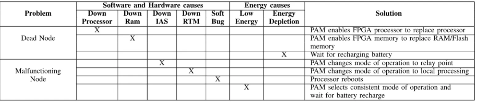
TABLE I
ISSUES AND CORRECTIVE SOLUTIONS FOR SENSOR NODE
Problem
Software and Hardware causes Energy causes
Solution
Down Down Down Down Soft Low Energy
Processor Ram IAS RTM Bug Energy Depletion
Dead Node
X PAM enables FPGA processor to replace processor
X PAM enables FPGA memory to replace RAM/Flash
memory
X Wait for recharging battery
Malfunctioning Node
X PAM changes mode of operation to relay point
X PAM changes mode of operation to local processing
X Processor reboots
X PAM selects consistent mode of operation and
wait for battery recharge TABLE II
OPERATING MODES OF SENSOR NODE
❳ ❳ ❳ ❳ ❳ ❳ ❳❳ Mode
Unit Processor RAM FPGA IAS RTM
Sensor1 Sensor2 Camera Transmitter Receiver
On-Duty On On Off On On/Off On/Off On On
Performance On On On On On/Off On/Off On On
Enhance
Dead Off On On On On/Off On/Off On On
Processor
Dead RAM On Off On On On/Off On/Off On On
Local On/Off On/Off On/Off On On/Off On/Off Off Off
Processing
Relay On/Off On/Off On/Off Off Off Off On On
Monitoring On/Off On/Off On/Off On Off Off Off On
Observation Sleep Off Off On Off Off Off On
Sleep Sleep Off Off Off Off Off Off Off
Deep Sleep Deep Sleep Off Off Off Off Off Off Off
Dead Node Off Off Off Off Off Off Off Off
problems encountered in a sensor node and their corrective solutions are described in Table I.
Apparently, our sensor node can react consistently against all issues with help of PAM and FPGA block. The first one is considered as the intelligent part for the best use of energy and fault-tolerance, while the other enhances the availability of sensor node. Besides, PAM block not only intervenes in case of failure, but also selects the suitable mode of operation to minimize the power consumption, that leads to extend the node lifetime. We define eleven operating modes for a sensor node including their active and inactive components, which are presented in Table II.
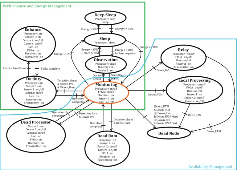
The behavior of node system refers to the Discrete Event System. Among all models, Finite State Machine (FSM) is suitable for modeling these operating modes (see Figure 4). This FSM model consists of a set of states and transitions. When each state represents a particular mode (On-Duty, Performance Enhance, Monitoring, Observation,...), and each transition represents one or more discrete events that make the transition from one operating mode to another one. The FSM model is divided into two parts marked with blue border and green rectangle. The blue one mentions the availability management of the system, while the green one relates to the compromise between performance and energy-efficiency. At beginning, FSM model enters in the Monitoring state, only Processor, Ram, Sensor1, and Receiver are active. In
the next sub-section, the first part of FSM model concerning the performance and energy management of sensor node is introduced.
C. Node Level Performance and Energy Management
By reason of limited powered battery, the energy-efficient consumption in sensor node is always one of major challenge for designer, even in case of auto-harvesting energy because the energy from the environment is generally unpredictable, discontinuous, and unstable. Additionally, the more energy is saved, the more node lifetime is extended. In our approach, sensor node can harvest energy from the environment by using Weather Forecasts (WFs) [6] model. WFs are used to determine which power harvesting source will have the highest energy availability and to predict the node lifetime. The energy management of our node is controlled by PAM block based on both DPM and DVFS policy [1], in which the first one can turn off the components while any task runs on them, and the second one can regulate the supply voltage and the operating frequency based on the type of generated event. In the Figure 4, the states are arranged in order of increasingly consuming energy such as Deep Sleep, Sleep, Observation, and Monitoring. Basing on the period of activities and the battery level, the state is changed between them.
As we know that most of the energy in WSN nodes is consumed by radio transceiver, but all the states (except Deep Sleep and Sleep) in our FSM model have receiver on, because we try to provide a general approach for all applications. For
Surveillance period Deep Sleep Processor : deep sleep Sleep Processor : sleep Energy < 5% Energy >= 10% Observation Processor : sleep Receiver : on Sensor 1 : on Energy >= 20% Energy < 15% Monitoring Processor : on/off FPGA : on/off Receiver : on Sensor 1 : on Ram : on/off Observe period On duty Processor : on Sensor 1 : on Sensor 2 : on/off Camera : on/off Ram : on Receiver : on Transmitter : on Detection alarm & !Down_Pro & !Down_Ram Enhance Processor : on Sensor 1 : on Sensor 2 : on/off Camera : on/off Ram : on FPGA : on Receiver : on Transmitter : on Operation completes Count > LimitCount Tasks complete
Dead Processor Sensor 1 : on Sensor 2 : on/off Camera : on/off Ram : on FPGA : on Receiver : on Transmitter : on Dead Ram Processor : on Sensor 1 : on Sensor 2 : on/off Camera : on/off FPGA : on Receiver : on Transmitter : on Relay Processor : on/off FPGA : on/off Ram : on/off Receiver : on Transmitter : on Local Processing Processor : on/off FPGA : on/off Ram : on/off Sensor 1 : on Sensor 2 : on/off Camera : on/off Dead Node Detection alarm & Down_Ram Operation completes Detection alarm & Down_Pro Operation completes (Down_RTM & Down_IAS) || (Down_Ram & Down_FPGAMem) || (Down_Pro & Down_FPGAPro) Down_RTM Down_IAS Down_IAS Down_RTM Energy < 15% || Sleep period Energy >= 20% & Observe period
Performance and Energy Management
Availability Management
Fig. 4. FSM model of operating modes for sensor node
example, in the application of detecting hazardous gaz for the normal area like warehouse, the radio transceiver is only turned on in a time interval based on the generated events. Thus, the sensor node switches mostly between Sleep, Monitoring and On-Duty modes. But with the same application for residential area, the radio receiver is always turn on, even in low power modes, to receive and send rapidly the data to the supervisor in case of detecting dangerous gaz. Therefore, the evacuation can be rapidly executed. In this application, the sensor node switches mostly between Observation, Monitoring and On-Duty modes to save energy.
Besides, the performance of the node system is also con-sidered to reduce the execution time of application. That leads to improve performance of the network. For example, the state is initially in Monitoring. When an alarm detection is generated, state changes to On-Duty, and Sensor2 or Camera can be turned on for image or video processing application. If the execution time of application passes a time deadline, PAM block activates the FPGA that allows parallel processing between processor and FPGA processor. Thus, this leads to accelerated execution. After completing all the tasks, the
system comes back to Monitoring state. The next sub-section describes availability management of our sensor node.
D. Node Level Availability Management
Definition III.1. Availability is the ability of an entity to be able to accomplish a required function under given conditions and at a given time.
As previously mentioned, the state of FSM model is ini-tially in Monitoring. When Sensor1 generates an alarm of detection and if the main processor is down, state changes to Dead Processor. Consequently, FPGA processor is enabled to replace the main one for processing the data. Some special devices such as Sensor2 or Camera can be turned on to verify the circumstance or take a video of the scene. After completing all tasks, the state comes back to Monitoring state. The procedure is similar when Ram memory is down, the FPGA memory is enabled, and state changes to Dead Ram if an alarming detection arrives. The other problems are considered such as failure of either the IAS or the RTM. The sensor node is considered as a relay point in the first case,
2 1 1 1 UpS DownS 2 FailS CapturedD ReadyDS StoreRam StoreFPGAMem UpRadio DownRadio FailRadio UpRam FailRam DownRam ActiveFPGAMem UpFPGAMem FailFPGAMem UpP FailP DownP ActiveFPGAP UpFPGAP FailFPGAP DownAllPro BeginBugP RebootP EndBugP BeginBugFPGAP RebootFPGAP EndBugFPGAP ComputeP ComputeFPGAP ReadyDRam 10 ReadyDP TransmitPack DownAllMem DownSenRadio FailSenRadio λs λram λfpgamem λp λfpgap λbug λbug λradio DataForTransmit StoreSentDataInRam StoreSentDataInFPGAMem
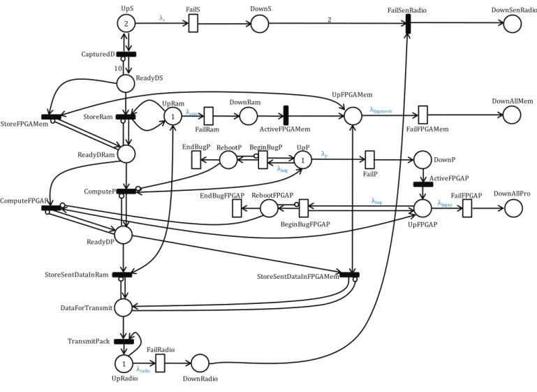
Fig. 5. GSPN availability model of sensor node for capturing data
or as local processing in second case. The local processing mode is defined because in some applications like detection of hazardous gaz, we keep the sensor node still running even when its radio module is failed. Thus, the technician can recover the recent captured data when he arrives to repair the radio module. If both sensors and radio transceiver, or main and FPGA processor, or RAM and FPGA memory are down, the node state reaches to Dead Node.
Since the behavior of node system refers to Discrete Event System, Petri Nets (PNs) [2] are suitable for modeling be-havior of communicating and synchronized processes. The availability of sensor node is modelled by Petri Nets (PNs), which not only performs the concurrent operations and asyn-chronous events of system, but also supports the failure pre-diction features. PN [5] is bipartite weighted graph including places(P:), transitions(T:). A transition is connected to its input places by input arcs shown as directional arrows. Conversely, output arcs drawn from the transitions to its output places. General Stochastic Petri Net (GSPN) [5] is used that supplies two types of transitions: timed transitions with exponentially distributed firing time and immediate transition with zero firing
time. Graphically, the places are described as circles, timed transitions as white rectangles, immediate transitions as black bars, tokens as dots or integer numbers within a place, arcs as lines with an arrow at end and inhibitor arcs as lines with small circles at end.
GSPN model of system of our node for capturing data is depicted in Figure 5. At beginning, several tokens reside in the places P:UpS, P:UpP, P:UpRam and P:UpRadio that represent the number of functioning components such as sensors, processor, ram memory and radio transceiver mod-ule. The failure rates of these components are respectively depicted by exponentially distributed firing rates λs, λp, λram,
λradio (see Table III). Appearance of a token in the places
P:DownS, P:DownP, P:DownRam and P:DownRadio indicates the failure of each component. When a data captured by sensors is stored in Buffer, a token is present in P:ReadyDS. An inhibitor arc with multiplicity of 10 from P:ReadyDS to T:CapturedD prevents the number of tokens in this place from being greater than 10, because capturing data buffer size is fixed to 10. Then, the data are stored in Ram memory before being processed by processor. If there is a software
bug with rate λbug during execution, the processor is re-booted. When processing is completed, a token is present in the P:ReadyDP meaning that data are ready for storing in memory before transmitting P:DataForTransmit. In case of failure of Ram memory or processor, FPGA memory or processor is activated for replacing. The failure rates of FPGA
memory and processor are respectively λf pgamem, λf pgap
(see Table III). Also, the inhibitor arcs from P:ReadyDRam to T:StoreRam and T:StoreFPGAMem, from P:ReadyDP to T:ComputeP and T:ComputeFPGAP, from P:DataForTransmit to T:StoreSentDataInRam and T:StoreSentDataInFPGAMem ensure that only one token can be in these places. On the other hand, the inhibitor arcs from P:RebootP to T:ComputeP and from P:RebootFPGAP to T:ComputeFPGAP mean that, while a processor is rebooting, computation cannot be performed.
The node system is completely down if a token appears in P:DownSenRadio or P:DownAllMem, or P:DownAllPro. It means that both IAS and RTM, or both Ram memory and FPGA memory, or both main Processor and FPGA Processor are down. Since we are focussing on the availability of the system, we can assume that the firing time for transitions T:CapturedD, T:StoreRam, T:StoreFPGAMem, T:ComputeP, T:ComputeFPGAP, T:TransmitPack, T:StoreSentDataInRam,
T:StoreSentDataInFPGAMem, T:ActiveFPGAMem,
T:ActiveFPGAP, T:FailSenRadio is small comparing to other activities. Thus, these transitions are modelled as immediate transitions (blacks bars), when others are modelled as timed transition (white rectangles). Because of the constraint of the paper length, the complete models of cluster and network are not presented here.
Several simulation results are exposed in section IV, that show the improvement in availability and consuming energy of sensor node, cluster, and network by applying our approach.
IV. SIMULATION RESULTS
The Stochastic Petri Net Package (SPNP) tool [8] is used for availability simulation tests. Mean Time To Failure (MTTF) is defined for each component.
Definition IV.1. Mean Time To Failure (MTTF) is defined for non-repairable systems to indicate the average functioning time from instance 0 to the first appearance of failure.
These MTTFs are shown in Table III. In this section, we do not simulate the software bug problem, we focus on the
TABLE III
FAILURERATE ANDMTTFFOR EACH COMPONENT
Component Failure rate (λ) Mean Time To Failure
Sensor 1/30000 fail/hour MTTF of a sensor is 3.4 years
Processor 1/262800 fail/hour MTTF of processor is 30 years
RAM 1/83220 fail/hour MTTF of RAM memory is 9.5
years
RTM 1/100000 fail/hour MTTF of radio transceiver is
11.4 years
FPGA memory 1/80000 fail/hour MTTF of FPGA memory is 9.1
years
FPGA processor 1/131400 fail/hour MTTF of FPGA processor is
15 years
failure of each component that is more serious. The time to occurence of failure in the Sensors, Ram memory, Processor and Radio module is assumed to be random variable with exponentially distributed rates λs, λram, λpand λradio(Table III). Since the failed components in our node can not be repaired, the availability of sensor node is computed as same as its reliability computation, A(t)= R(t).
Definition IV.2. Failure rate λ(t) is the limit, between t and t+dt , of the quotient of the probability density of failure by the probability of reliability before t.
λ(t) = 1 R(t). dF(t) dt = 1 R(t). −dR(t) dt = f(t) R(t), F(t) = 1−R(t) (1) We have the probability density of failure:
f(t) =dF(t)
dt = −
dR(t)
dt (2)
and f(t)dt is the failure probability of the entity between t and t+dt:
f(t)dt = P r[t < T < t + dt] (3)
While λ(t)dt is the failure probability of the entity during interval [t, t+dt], given the fact that the entity has not been failed during interval [0, t], hence:
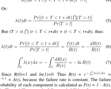
λ(t)dt = P r[t < T < t + dt|T > t] (4) Or: λ(t)dt = P r[(t < T < t + dt)T(T > t)] P r[T > t] (5) But (T > t)T (t < T < t+dt) = (t < T < t+dt), thus: λ(t)dt = P r[(t < T < t + dt)] P r[T > t] = f(t).dt R(t) = − dR(t) R(t) (6) Z t 0 λ(x) dx = − Z t 0 dR(x) R(x) = − ln R(t) (7)
Since R(0)=1 and ln(1)=0. Thus R(t) = e−R0tλ(x) dx =
e−λ.t = A(t)
, because the failure rate is constant. The failure probability of each component is calculated as F(t) = 1 - A(t). The Figure 6 illustrates the failure probabilities of components over ten years, in which the sensors are the most critical components due to their low reliability (the smallest MTTF), because their circuitry is very complex.
In SPNP tool, we can define the appropriate reward rates to compute the output mesures of interest. The advantage is that we only need to specify the reward rates associated with certain conditions of the system, instead of explicitly identifying all its states. In our case, the availability of node system is the output mesure of interest. Node system is still available if there is not any token in P:DownSenRadio, or P:DownAllMem, or P:DownAllPro (see Figure 5). To compute the availability of node system by using SPNP tool, we only
Probability
Time (years) Failure probability of sensors Failure probability of Ram Failure probability of Radio transceiver Failure probability of Processor
Fig. 6. Failure probability of components
Availability
Time (Years) 0,31
0,09
Sensor node without PAM block and FPGA Sensor node with PAM block and FPGA
Fig. 7. Comparison of node availability with and without our approach
need to specify reward rate associated with the condition of node availability as follows:
ravailability= 0 if (#(DownSenRadio)=1) or (#(DownAllMem)=1) or (#(DownAllPro)=1). 1 otherwise. (8)
Where: #(p) represents the number of tokens in place p.
The availability of our node at time t is computed as the expected instantaneous reward rate E[X(t)] at time t, where X(t) is a random variable corresponding to the instantaneous reward rate of node availability. The expression of E[X(t)] is described as follows:
E[X(t)] =X
k∈T
rk.πk(t) (9)
πk(t) is the probability of being in marking k at the time
t, and T is the set of markings. The computation of πk(t)
is described in detail in [5]. The Figure 7 depicts that the node availability is significantly increased from 9% to 31% over twelve years. From node availability results, the cluster availability is then simulated. We assume that our sensor
Time (Years) 0,46
0,09 Availability
Sensor cluster without PAM block and FPGA Sensor cluster with PAM block and FPGA
Fig. 8. Comparison of cluster availability with and without our approach
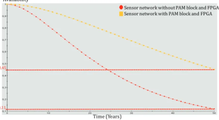
Time (Years)
0,45
0,11
Availability
Sensor network without PAM block and FPGA Sensor network with PAM block and FPGA
Fig. 9. Comparison of network availability with and without our approach
cluster consists of two normal nodes, a Gateway and a Can-didate Gateway. Figure 8 presents the comparison of cluster availability simulation with and without using our device, and Candidate Gateway. Cluster availability is increased from 9% to 46% over eighteen years with our approach. Also, the im-pact of our approach is tested in network availability. Similarly, we assume that our network consists of two clusters, a Sink and a Relief Sink. Figure 9 introduces a large improvement in network availability from 11% to 45% over fifty years.
In the energy simulation, our approach is tested with the ap-plication of hazardous gaz detection for area such as harbor or warehouse. Our sensor node has a PIC24FJ256GB110 MCU, a M48T35AV RAM memory, a Miwi radio transceiver, a Oldham OLCT 50 gaz detection, the power switches (LM3100 and MAX618), and a battery. Our energy management is based
TABLE IV
ENERGY CONSUMPTION OF EACH COMPONENT IN SEVEN DAYS
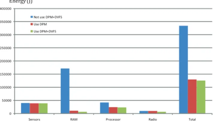
Components Non DPM+DVFS(kJ) DPM(kJ) DPM+DVFS(kJ) Sensors 39.673 39.151 39.225 RAM 171.73 10.545 6.277 Processor 41.671 24.047 23.123 Radio 9.956 9.824 6.205 Total 334.3 129.173 125.519
0 50000 100000 150000 200000 250000 300000 350000 400000
Sensors RAM Processor Radio Total
Not use DPM+DVFS Use DPM Use DPM+DVFS Energy (J)
Fig. 10. Comparison of consuming energy of node with and without our
approach
on DPM and DVFS policies. Three simulations with duration of seven days are realized by using CAPNET Power Energy Estimator software [6] that has been developped by our Lab-STICC laboratory. In the first one, the DPM and DVFS policies are not used, it means that the MCU and the RAM memory are at Monitoring modes in all the functioning time, and the other components run at their maximum supply voltage when being activated. In the second one, only DPM is used to turn off the MCU and the RAM memory when there is not any running task. For the last simulation, both DPM and DVFS are used. The supply voltage and the operating frequency is dynamically regulated for each component based on the type of generated event. To mitigate the large overheads in computation by using DVFS, the supply voltage is set maximum for each component in case of hazardous gaz detection, and is set minimum for each component when any detection is found. The energy consumption of each component is given in the Table IV. In this table, the total energy consumption represents the sum of the energy being consumed by all the components and the energy loss in all the converters. These results indicate that the total energy being consumed by the third simulation is 62.5% less than the first one, and is 3.2% less than the second one (as depicted in Figure 10). In this paper, the consumption of PAM is ignored since we have not decided its hardware configuration. Additionally, PAM only checks the state of other components by polling periodically the components, it does not realize any complex computation. Thus, our PAM device occupies very small space and consumes very small energy compared with other component. The PAM consumption will be mesured in our future works.
V. CONCLUSIONS AND PERSPECTIVES In this paper, a design of WSN node for increased avail-ability and energy-efficiency is presented. An original device named Power Availability Management (PAM) combined with FPGA is employed. FSM and GSPN models are used to evaluate the availability and energy consumption of sensor node. The simulation results with Capnet-PE and SPNP tool show that our approach significantly increases the availability and energy-saving of sensor node, which allows to lead to a more reliable and energy-efficient sensor cluster and network.
Finally, we have demonstrated the feasibility and interest of our approach and we will implement it on a real case in order to validate with the measurements. Our future works focus on the following aspects:
• A Time Division Multiple Access (TDMA) method [3] is
allocated or created in order to avoid the buffer overflow problem that leads to a steady connection between nodes.
• As we know, the data transmission is the most
consum-ing part of battery energy. Therefore, Dynamic Voltage Frequency Scaling (DVFS) can be applied to set different operating frequency for transmission according to the size of data. That leads to a energy-efficient transmission.
• In case of Gateway failure, many strategies can be
considered to select a new Gateway like the most reliable transmission Candidate Gateway, or Candidate Gateway that possesses the highest residual energy, or combined both two aspects.
The author would like to express his sincere thanks to Mr. Kishor S. Trivedi (Hudson Professor of Electrical and Com-puter Engineering), and Mr. Xiaoyan Yin (Technical Engineer of Electrical and Computer Engineering) at Duke University, USA for providing SPNP tool and helping us to use it.
The author is greatly thankful to his colleague Nicolas Ferry, one of the authors of CAPNET-PE Estimator tool, for his very helpful support during the energy simulation.
REFERENCES
[1] Marcus T. Schmitz, Bashir M. Al-Hashimi, Petru Eles, System-Level Design Techniques for Energy-Efficient Embedded Systems, Kluwer Aca-demic Publishers, first edition, Boston, USA, 2004.
[2] S. Lafortune, C.G. Cassandras, Introduction to Discrete Event System, Springer Publishers, second edition, Harvard, USA, 2008.
[3] R. Karri, D. Goodman, System-Level Power Optimization for Wireless Multimedia Communication, Kluwer Academic Publishers, first edition, Dordrecht, The Netherlands, 2002.
[4] C. Constantinescu, Dependability evaluation of a fault-tolerant processor by GSPN modeling, IEEE Transactions on Reliability, September, 2005, pp. 468–474.
[5] P. Chimento , JR. Jogesh , K. Muppala , G. Ciardo , A. Blakemore and K.S. Trivedi, Automated generation and analysis of markov reward models using stochastic reward nets, Linear Algebra, Markov Chains and Queuing Models, Eds: Springer Verlag, 1993, pp. 145–191.
[6] Nicolas Ferry , Sylvain Ducloyer , Nathalie Julien and Dominique Jutel, Power/Energy Estimator for DesigningWSN Nodes with Ambient Energy Harvesting Feature, EURASIP Journal on Embedded Systems, January , 2011.
[7] M.A. Lopez-Gomez, J.C. Tejero-Calado, A lightweight and energyeffi-cient architecture for wireless sensor networks, IEEE Transactions on Consumer Electronics, August, 2009, pp. 1408–1416.
[8] J. Muppala , G. Ciardo, K.S. Trivedi, Spnp: Stochastic petri net package, Proceedings of the Third International IEEE Workshop, 1989, pp. 142– 151.
[9] M. Ringwald, K. Romer, Deployment of sensor networks: Problems and passive inspection, Fifth IEEE Workshop on Intelligent Solutions in Embedded Systems, June, 2007, pp. 179–192.
[10] J. Suhonen, M. Hanninen, T.D. Hamalainen, M. Hannikainen, Remote diagnostics and performance analysis for a wireless sensor network, IEEE Workshop on Signal Processing Systems (SiPS), October, 2011, pp. 67– 72.
[11] K. Romer, M. Ringwald, A. Vitaletti, Snif: Sensor network inspection framework, ETH Zurich, Zurich, 2006.
[12] H. Hassanein, Jing Luo, Reliable energy aware routing in wireless sensor networks, Second IEEE Workshop on Dependability and Security in Sensor Networks and Systems (DSSNS), April, 2006, pp. 54–64.