HAL Id: hal-00184991
https://hal.archives-ouvertes.fr/hal-00184991
Submitted on 4 Nov 2007HAL is a multi-disciplinary open access archive for the deposit and dissemination of sci-entific research documents, whether they are pub-lished or not. The documents may come from teaching and research institutions in France or abroad, or from public or private research centers.
L’archive ouverte pluridisciplinaire HAL, est destinée au dépôt et à la diffusion de documents scientifiques de niveau recherche, publiés ou non, émanant des établissements d’enseignement et de recherche français ou étrangers, des laboratoires publics ou privés.
Singular Curves in the Joint Space and Cusp Points of
3-RPR parallel manipulators
Mazen Zein, Philippe Wenger, Damien Chablat
To cite this version:
Mazen Zein, Philippe Wenger, Damien Chablat. Singular Curves in the Joint Space and Cusp Points of 3-RPR parallel manipulators. Robotica, Cambridge University Press, 2007, 25 (6), pp.717-724. �10.1017/S0263574707003785�. �hal-00184991�
1
S
INGULARC
URVES IN THEJ
OINTS
PACE ANDC
USPP
OINTS OF3-RPR
PARALLEL MANIPULATORSMazen ZEIN, Philippe Wenger and Damien Chablat
Institut de Recherche en Communications et Cybernétique de Nantes UMR CNRS 6597 1, rue de la Noë, BP 92101, 44312 Nantes Cedex 03 France
E-mail address: Mazen.Zein@irccyn.ec-nantes.fr
Phone: 0033240376955 Fax: 0033240376930
Abstract
This paper investigates the singular curves in the joint space of a family of planar parallel manipulators. It focuses on special points, referred to as cusp points, which may appear on these curves. Cusp points play an important role in the kinematic behavior of parallel manipulators since they make possible a nonsingular change of assembly mode. The purpose of this study is twofold. First, it exposes a method to compute joint space singular curves of 3-RPR planar parallel manipulators. Second, it presents an algorithm for detecting and computing all cusp points in the joint space of these same manipulators.
1. Introduction
Because at a singularity a parallel manipulator loses its stiffness, it is of primary importance to be able to characterize these special configurations. This is, however, a very challenging task for a general parallel manipulator1. Planar parallel manipulators have received a lot of attention1-8 because of their relative simplicity with respect to their spatial counterparts. Moreover, studying the former may help understand the latter. Planar manipulators with three extensible leg rods, referred to as 3-RPR manipulators, have often been studied. Such manipulators may have up to six assembly modes7. The direct kinematics can be written in a polynomial of degree six3. Moreover, as is the case in most parallel manipulators, the singularities coincide with the set of configurations where two direct kinematic solutions coincide. It was first pointed out that to move from one assembly
2 mode to another, the manipulator should cross a singularity7. However, Innocenti8 showed, using numerical experiments, that this statement is not true in general. More precisely, this statement is only true under some special geometric conditions, such as similar base and mobile platforms9,10. In fact, an analogous phenomenon exists in serial manipulators that can change their posture (inverse kinematic solution) without meeting a singularity in general, but not under special geometric simplifications8,11-13. The nonsingular change of posture in serial manipulators was shown to be associated with the existence of points in the workspace where three inverse kinematic solutions meet, called cusp points13. Cusp points in serial manipulators were determined by looking for the triple roots of the inverse kinematics polynomial13 or from the equation of the workspace boundary14. Likewise, McAree9 pointed out that for a 3-RPR parallel manipulator (as well as for its spatial counterpart, the octahedral manipulator), if a point with triple direct kinematic solutions exists in the joint space, then the nonsingular change of assembly mode is possible. A condition for three direct kinematic solutions to coincide was established. However, no systematic exploitation of this condition was possible because the algebra involved was too complicated and to the authors’ knowledge, the work of McAree9 has never been pursued yet. Wenger15 showed that to accomplish a non-singular assembly-mode changing motion, a 3-RPR manipulator platform should encircle a cusp point in its joint space. Thus, determination of cusp points is of interest for planning trajectories. A procedure for computing joint space singularities of 3-RPR parallel manipulators was established in a previous paper16, where the cusp points were shown on the joint space singularities of these manipulators but no solution was proposed for computing these cusp points.
In this paper, the abovementioned condition for computing cusp points is reviewed and exploited. An algorithm for the systematic detection of cusp points is developed. The method16 for computing and representing joint space singularities of 3-RPR planar parallel manipulators is first recalled. A descriptive analysis of the singular curves in slices of the joint space of 3-RPR parallel manipulators is conducted. It is shown that the number of cusp points depends on the slice of the
3 joint space in which these cusp points are determined. Moreover, the maximum number of cusp points depends on the geometry of the manipulator. This work helps better understand the topology of the joint space of parallel manipulators and finds applications in both design and trajectory planning.
The following section introduces the 3-RPR manipulator and its constraint equations. Section 3 is devoted to the determination of the singular curves in slices of the joint space. The existence condition of cusp points is derived in section 4 and an algorithm to determine these points automatically is provided. Section 6 is devoted to a descriptive analysis of singular curves in slices of the joint space.
2. Preliminaries
2.1 Manipulators under study
The manipulators under study are 3-DOF planar parallel manipulators with three extensible leg rods (Fig. 1). These manipulators have been frequently studied4-8. Each of the three extensible leg rods is actuated with a prismatic joint. The geometric parameters of the manipulators are the three sides of the moving platform d1, d2, d3 and the position of the base revolute joint centers defined by
A1, A2 and A3. The reference frame is centered at A1 and the x-axis passes through A2. Thus, A1 = (0,
0), A2 = ( A2x , 0) and A3 = ( A3x , A3y). x A1 A2 B2 B3 B1 θ ρ1 ρ2 θ2 d1 d3 d2 θ1 y A3 ρ3 θ3 α β h
4
2.2 Constraint equations
Let L ≡ (ρ1, ρ2, ρ3) define the lengths of the three leg rods and let θ ≡ (θ1, θ2, θ3) define the
three angles between the leg rods and the x-axis. The six parameters (L, θ) can be regarded as a configuration of the manipulator but only three of them are independent, so that the configuration space is a 3-dimensional manifold embedded in a 6-dimensional space. The dependency between (L, θ) can be identified by writing the fixed distances between the three vertices of the mobile platform B1, B2, B3:
[
] [
]
[
] [
]
[
] [
]
2 1 2 1 2 1 1 2 2 3 2 3 2 2 2 3 1 3 1 3 3 ( , ) ( , ) ( , ) ( , ) ( , ) 0 ( , ) ( , ) ( , ) ( , ) ( , ) 0 ( , ) ( , ) ( , ) ( , ) 0 ( , ) T T T d d d ⎧ Γ = − − − = ⎪⎪Γ = − − − = ⎨ ⎪ Γ = − − − = ⎪⎩ L θ b L θ b L θ b L θ b L θ L θ b L θ b L θ b L θ b L θ L θ b L θ b L θ b L θ b L θ (1)where bi is the vector defining the coordinates of Bi in the reference frame as function of L and
θ. For more simplicity, (L, θ) will be omitted in the following equations. Expanding each Γi as a series about the configuration (L, θ) yields
2 3 3 3 3 1 1 1 1 3 3 1 1 2 .. 0 1 ... ! 1 ! i i i i i i i j j j j j j j j n i i i j j j j n θ θ θ ρ θ ρ θ θ ρ
ρ
ρ
ρ
= = = = = = ⎛ ∂ ∂ ⎞ ⎛ ∂ ∂ ⎞ ΔΓ =⎜⎜ Δ + Δ ⎟⎟Γ + ⎜⎜ Δ + Δ ⎟⎟ Γ ∂ ∂ ∂ ∂ ⎝ ⎠ ⎝ ⎠ ⎛ ∂ ∂ ⎞ Δ + Δ Γ + = ⎜ ⎟ ⎜ ∂ ∂ ⎟ ⎝ ⎠ + +∑
∑
∑
∑
∑
∑
(2)If one keeps only the first-order and second-order terms, Eq.(2) can be written in matrix form as follows: 2 2 2 1 1 1 2 2 2 2 2 2 2 2 2 2 2 2 2 3 3 3 2 2 1 1 0 2 2 T T T T T T T T T ⎡ ∂ Γ ⎤ ⎡Δ ∂ Γ Δ ⎤ Δ Δ ⎡Δ ∂ Γ Δ ⎤ ⎢ ⎥ ⎢ ∂ ⎥ ∂ ∂ ⎢ ∂ ⎥ ⎢ ⎥ ⎢ ⎥ ⎢ ⎥ ⎢ ⎥ ∂ ∂ ⎢ ∂ Γ ⎥ ∂ Γ ⎢ ∂ Γ ⎥ Δ = Δ + Δ + ⎢Δ Δ + Δ⎥ ⎢ Δ ⎥+ ⎢Δ Δ ⎥= ∂ ∂ ⎢ ∂ ⎥ ⎢ ∂ ∂ ⎥ ⎢ ∂ ⎥ ⎢ ⎥ ∂ Γ ∂ Γ ⎢Δ Δ ⎥ ∂ Γ ⎢Δ Δ ⎥ ⎢Δ Δ ⎥ ⎢ ∂ ⎥ ∂ ∂ ⎢ ∂ ⎥ ⎣ ⎦ ⎢⎣ ⎥⎦ ⎣ ⎦ θ L θ θ L L θ L θ L Γ Γ Γ θ L θ θ θ L L L θ L θ θ L L θ θ θ L L L θ θ L L (3)
Equation (3) can be used to describe an arbitrary local motion at a given configuration of the manipulator9. When first order terms of Eq.(3) are sufficient to describe the motion, the manipulator
5 is in a regular configuration and the following equation (4) can be used instead of Eq.(3):
(
,)
(
,)
0 ∂ ∂ Δ + Δ = ∂ ∂ Γ L θ Γ L θ θ L θ L (4)Otherwise the configuration (L,θ) is special and the manipulator meets a singularity. This happens when the constraint Jacobian ∂ ∂Γ/ θ drops rank so that the second order terms of equation (3) are required to describe the constraints. The three vertices of the moving platform have the following coordinates in the fixed reference frame,
( )
( )
( )
( )
( )
( )
1 1 1 1 1 2 2 2 2 2 2
3 3 3 3 3 3 3
cos sin ; cos sin ;
cos sin . T T x T x y A A A ρ θ ρ θ ρ θ ρ θ ρ θ ρ θ =⎡⎣ ⎤⎦ =⎡⎣ + ⎤⎦ ⎡ ⎤ =⎣ + + ⎦ b b b
Thus, the constraint Jacobian can be put in the following form:
(
)
(
)
(
)
(
)
1 2 1 2 12 2 1 21 2 2 2 2 3 2 3 2 3 3 3 23 3 2 2 23 3 3 1 3 1 3 31 3 3 3 1 31 3 1 3 3 0 ( ) ( ) 2 0 ( ( 0 ) ) x x x x x x y y x x y y A s s s A s A A s A A s s A c s A c A s s A s s A c A c ρ ρ ρ ρ ρ ρ ρ ρ ρ ρ ρ ρ ⎡ ⎤ ⎢ + − ⎥ ⎢ ⎥ ⎢ ⎥ − − − ⎢ ⎥ ∂ = ⎢ ⎥ ∂ ⎢ − + − + ⎥ ⎢ ⎥ ⎢ − − − ⎥ ⎢ − − ⎥ ⎢ ⎥ ⎣ ⎦ Γ θ (5)wheresi =sin
( )
θi , ci =cos( )
θi and sij =sin(
θ θi− j)
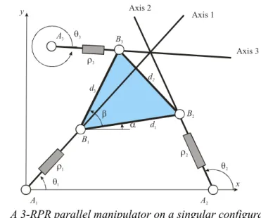
. 3. Jointspace Singular CurvesThe manipulator is in a singular configuration whenever the axes of its three leg rods are concurrent or parallel17.
6 x A1 A2 B1 θ2 θ1 y A3 θ3 B2 B3 d1 d3 d2 α β Axis 1 Axis 3 Axis 2 ρ2 ρ1 ρ3
Fig 2. A 3-RPR parallel manipulator on a singular configuration
We derive the condition for the three leg axes to intersect at a common point (possibly at infinity). We first write the equations of the three leg axes:
1 1
2 2 2
3 3 3 3 3
(Axis 1) : cos( ) sin( )
(Axis 2) : cos( ) ( )sin( )
(Axis 3) : cos( ) ( )sin( ) cos( )
x x y y x y x A y x A A θ θ θ θ θ θ θ ⎧ = ⎪ = − ⎨ ⎪ = − + ⎩ (6) Eliminating x and y in (6) yields the following singularity equation in the task parameters (θ1,
θ2, θ3):
(
)
2x 2 31 3x 3 3y 3 12 0
A s s + A s −A c s = (7)
where si =sin
( )
θi , ci =cos( )
θi and sij =sin(
θ θi− j)
.It is possible to express Eq (7) as function of the joint space parameters ρ1, ρ2 and ρ3 by using
the constraint equations of the 3-RPR manipulator. However, the resulting equation would be too complicated to yield real insights and difficult to handle. Our approach to compute the singular configurations in the joint space consists in reducing the dimension of the problem. We consider two-dimensional slices of the configuration space by fixing the first leg rod length ρ1.
Step 1: We rewrite Eq. (7) as a function of ρ1, α and θ1 using the constraint equations of the
7
( )
( )
(
)
(
)
2 2 2 1 1 1 2 2 1 1 1 3 3 3 1 1 3 3 3 3 1 1 3 c c cos 0 s s sin 0 c c cos 0 s s sin 0, x x y A d d A d A d ρ ρ α ρ ρ α ρ ρ α β ρ ρ α β + − − = ⎧ ⎪ − − = ⎪ ⎨ + − − + = ⎪ ⎪ + − − + = ⎩ (8)The first (resp. last) two equations make it possible to express ρ2 (resp. ρ3) as function of ρ1, α
and θ1. Then, c2 and s2 (resp. c3 and s3) are calculated as function of ρ1, α and θ1 from the first (resp.
last) two equations of (8) and their expressions are input in Eq. (7), which, now, depend only on ρ1,
α and θ1.
Step 2: We fix a value for ρ1, so Eq. (7) depends now only on α and θ1. By varying α or θ1, we
compute the roots of the equation, to obtain the singular configurations (αs, θ1s) for a fixed ρ1s.
Step 3: For every singular configuration computed in the second step of the approach, we
calculate the corresponding values ρ2s and ρ3s using equation system (9). We have thus the singular
configurations curves in a slice of the joint space (ρ2, ρ3) for a fixed value of ρ1:
(
)
(
)
(
)
(
)
2 2 1 1 1 2 2 1 1 1 2 3 1 1 3 3 2 3 1 1 3 cos( ) cos( ) sin( ) sin( ) cos( ) cos( ) sin( ) sin( ) x x y A d d A d A d ρ θ α ρ ρ θ α ρ θ α β ρ ρ θ α β ⎧ − + + + ⎪ = ⎪ + ⎪ ⎨ ⎪ − − + + ⎪ = ⎪ − − + ⎩ (9)Figure 3 shows a slice of the joint space singular configurations for ρ1=17 obtained for the
same 3-RPR manipulator used by several authors 1,8,9, which has the following geometric parameters: A1= (0, 0), A2= (15.91,0), A3 = (0, 10), d1= 17.04, d2= 16.54 and d3 = 20.84 in an
8
Fig 3. Singular curves in (α, θ1) for ρ1=17. Number of assembly modes is displayed in each region
Figure 3 shows the singular curves in the joint space slice (ρ2, ρ3) defined by ρ1=17. These
curves give rise to several regions with 2, 4 or 6 direct kinematic solutions. The six points pinpointed with circles are cusp points, where three direct kinematic solutions coincide.
4. Determination of the Cusp Points
4.1 Existence condition of cusp points
For serial 3-DOF manipulators, the cusp points can be determined by deriving the condition under which the inverse kinematics polynomial admits three identical roots13. However this
approach is much more complicated when applied to the direct kinematics polynomial of 3-RPR manipulators because this polynomial is of degree 6.
An interesting alternative approach was proposed in McAree’s study9 by writing the condition under which the manipulator loses first and second order constraints. The resulting condition for triple coalescence of assembly modes was shown to take the following form:
2 2 2 3 1 2 1 2 2 2 3 2 0, T ⎡u ∂ Γ +u ∂ Γ +u ∂ Γ ⎤ = ⎢ ∂ ∂ ∂ ⎥ ⎣ ⎦ v v θ θ θ (10)
9 components of the unit vector uthat spans the left kernel. Vectors uand vcan be chosen in the set of nonzero rows and columns of the adjoint of matrix ∂ ∂Γ/ θ(i.e. the matrix of cofactors of the transpose of ∂ ∂Γ/ θ), respectively.
Calculating the adjoint of ∂ ∂Γ/ θ from Eq. (5) yields:
adj 1 2 2 5 3 5 3 4 2 6 3 6 1 4 4 5 1 6 k k k k k k k k k k k k k k k k k k − ⎛ ⎞ ∂ ⎛ ⎞ ⎜= ⎟ ⎜∂ ⎟ ⎜ ⎟ ⎝ ⎠ ⎜− ⎟ ⎝ ⎠ Γ θ (11) where
(
)
(
)
(
)
(
)
(
)
1 2 3 2 2 3 23 3 2 2 3 1 13 3 3 3 3 3 3 3 2 3 2 23 3 3 2 2 2 x x y x y x x y k A A s s A c k s A s A c k A A s s A c ρ ρ ρ ρ ρ ρ = − + − = − + − = − − + −(
)
(
)
(
)
4 1 3 13 3 1 3 1 5 2 1 12 2 2 6 1 2 12 2 1 2 2 2 x y x x k s A s A c k s A s k s A s ρ ρ ρ ρ ρ ρ = + − = − + = + (12)Taking u (resp. v) as the first row (resp. column) of (11), Eq. (10) can be written as
(
)
2 1 2 2 2 3 1 2 1 2 3 4 1 4 1 2 2 2 5 2 3 5 2 3 4 1 4 0 k k k k k k k k k k k k k k k k k k ⎛ ⎞ ⎛ ∂ Γ ∂ Γ ∂ Γ ⎞⎜ ⎟ − ⎜ − + ⎟⎜ ⎟= ∂ ∂ ∂ ⎝ θ θ θ ⎠⎜⎝− ⎟⎠ (13) where(
)
(
)
(
)
(
)
(
)
2 1 2 1 2 21 1 2 21 1 1 2 21 2 2 2 1 21 2 2 2 2 3 2 2 2 3 23 2 3 23 3 2 3 2 3 3 2 3 23 2 23 3 3 1 3 1 3 31 3 1 1 3 2 3 2 0 2 0 0 0 0 0 0 0 ( ) 2 0 ( ) 0 0 2 x x x x y x x y x y A c c c c A c c A A c c c A s A A c c c A s A c c A s ρ ρ ρ ρ ρ ρ ρ ρ ρ ρ ρ ρ ρ ρ ρ ρ ρ ρ ρ ρ + − ⎡ ⎤ ∂ Γ = ⎢ − − − ⎥ ∂ ⎢⎣ ⎥⎦ ⎡ ⎤ ⎢ ⎥ ⎢ ⎥ − − ⎢ ⎥ ∂ Γ = ⎢ − ⎥ − − ∂ ⎢ ⎥ ⎢ − ⎥ − ⎢ ⎥ + − ⎢ ⎥ ⎣ ⎦ + + − ∂ Γ = ∂ θ θ θ(
)
31 1 3 31 3 1 31 3 3 3 3 0 0 0 0 x y c c c A c A s ρ ρ ρ ρ ⎡ ⎤ ⎢ ⎥ ⎢ ⎥ − − − ⎢ ⎥ ⎣ ⎦ (14)In McAree’s study9, Eq. (13) was not expanded. McAree9 noted that the expansion of this equation was too complicated to yield any real insight.
10 implemented it in Maple. This algorithm detects all the cusp points inside the joint space of any
3-RPR manipulators and computes their coordinates. We present it in next section. 4.2 Algorithm for calculating cusp points
The presence of cusp points allows the 3-RPR manipulator to undertake non-singular assembly mode changing trajectories; these special trajectories can be executed by encircling a cusp point. In their study9, the authors stated that cusp points are pernicious and should be avoided or designed out by judicious dimensioning.
The configuration of the 3-RPR manipulator is given by six parameters: the three rod lengths (ρ1, ρ2, ρ3), and the platform position variables (θ1, θ2, θ3). Only three of these parameters are
independent. In order to reduce the dimension of the problem, McAree9 shows that it is possible to consider two-dimensional slices of the configuration space by fixing one of the leg rod lengths.
By doing so, the manipulator configuration can be fully defined by only two parameters. For example, for a fixed value of ρ1, a configuration may be fully defined by either (α,θ1) or (ρ2, ρ3).
Note that in the first case, the configuration is defined in the output space by the position and the orientation of the moving platform (ρ1 and θ1 define the position of B1 in the plane and α defines the
orientation of the moving platform in the plane). In the second case, the configuration is defined in the joint space by the lengths of the three leg rods.
In our work, we have always taken ρ1 as the fixed parameter. After fixing the value of ρ1, we
first calculate the singularity curves in (ρ2, ρ3), and then we compute all the cusp points of this
two-dimensional slice.
4.2.1 Algorithm
If we consider equation (7), we notice that it is a function of (θ1, θ2, θ3). The existence
condition of cusp points (13) is a function of (ρ1, ρ2, ρ3) and (θ1, θ2, θ3). Our first goal is to establish
an equation, which is a function of (ρ1, α, θ1), and then to solve it to obtain the coordinates of the
11
( )
( )
( )
( )
( )
(
)
( )
( )
( )
( )
( )
(
)
2 1 1 1 2 2 3 1 1 3 3 3 1 1 1 2 2 3 1 1 3 3 3 cos cos cos cos cos s sin sin sin sin sin sin x x y A d A d co d A d ρ θ α θ ρ ρ θ α β θ ρ ρ θ α θ ρ ρ θ α β θ ρ ⎧ − + + = ⎪ ⎪ ⎪ − + + + = ⎪ ⎪ ⎨ + ⎪ = ⎪ ⎪ − + + + ⎪ = ⎪ ⎩ (15)The algorithm for detecting cusp points is implemented in MAPLE; its steps are presented below:
1. First, the expression of cos(θ2), cos(θ3), sin(θ2) and sin(θ3) in (15) are substituted into the
singularity equations (7). Then, sin(α) and cos(α) (resp. cos(θ1) and sin(θ1)) are written as
function of tan(α/2) (resp. of tan(θ1/2)). As a consequence we obtain an equation of the
form:
(
)
1 1, ,1 0
F ρ t t = (16)
where t=tan
( )
α and t1 =tan( )
θ1 .2. Then, the expression of cos(θ2), cos(θ3), sin(θ2) and sin(θ3) in (15) are substituted into
equations (12) and (14). Applying then the tan-half substitution as above yields an equation of the form:
(
)
1 1, , 1 0
E ρ t t = (17)
So, we notice that the two equations (7) and (13) are written now as function of three parameters only.
3. We fix now ρ1, and we input the manipulator parameters d1, d2, d3, A2x, A3x and A3y. We have
noticed that the direct substitution of the real values of sin
( )
β and cos( )
β into equations12 we write sin
( )
β and cos( )
β as a function of an intermediate parameter h, which is thealtitude of the moving triangle.
4. The Maple resultant function is used to eliminate t =tan
( )
α from the two equations (16)and (17). The resulting equation is a polynomial of degree 96 in t1=tan
( )
θ1 , which can be factored as follows: 3 1 1 2 1 2 3 ... n1 n 0 a a a a a n n P P P P P Q− − = (18)where Q is a 24th-order univariate polynomial in t1 and P1, P2,…,Pn are quadratic and quartic
polynomials in t1. Note that the factor form could not be obtained without the intermediate
parameter h.
5. We input the parameter h value. We solve equation (18). Each real root t1i is
back-substituted into (16), which is then solved for t. For every t1i, we obtain different values for
tij. Finally, we get a number of solution couples (tij,t1i).
6. We substitute the values of each solution couple (tij,t1i) into (17), and we keep only those
solutions that satisfy this equation.
The solutions (tij,t1i) kept in the last step should give the coordinates of the cusp points. To
verify this, we calculate the direct kinematic solutions for each solution (tij,t1i). In many
instances, we have found that some solutions do not yield three coincident solutions. This means that they are not associated with cusp points. So we reject them and we keep only those solutions that give three coincident direct kinematic solutions. These couples are the coordinates of the cusp points, we call them (αij,θ1i)cusp.
After running our algorithm hundreds of times, we have noticed that in each case all cusp points were determined by the 24th-order polynomial Q of equation (18), that is, all remaining factors provided spurious solutions. Thus, we may conjecture that the cusp points are determined by
13 With this conjecture, our algorithm simplifies significantly because instead of solving (18) (a 96th order polynomial), we just have to solve polynomial Q (a 24th order polynomial).
To implement this result in the algorithm, we must change steps 5 and 6 into the following steps 5’ and 6’, and eliminate step 7:
5'. We input the real value of parameter h. We solve the polynomial Q. We substitute every real root θ1i of Q into equation (16), and solve it for tan(α/2). For every θ1i, we obtain different
values αij. Finally, we get a number of couples (αij,θ1i).
6'. We substitute the values of each couple (αij,θ1i) into equation (17). The couples that satisfy
this equation are the coordinates of the cusp points. We call them (αij,θ1i)cusp.
Finally, to obtain the coordinates of the cusp points in the joint space (ρ1, ρ2, ρ3), we use the
system of equations (9) computed from the geometry of the manipulator. We then obtain the cusp points in a slice of the joint space for a fixed value of ρ1.
In step 7 of the algorithm, we have noticed that the existence condition of cusps generates solutions that do not provide triple direct kinematic solutions. This confirms the statement of McAree9 that the cusp existence condition that he established is a sufficient condition but not a necessary one.
4.2.2 Algorithm Execution
The algorithm execution time slightly depends on the value of ρ1 and of the 3-RPR manipulator
parameters. It highly depends on the number of digits required for the calculation. For 90 digits (which is necessary to guaranty a good accuracy), it is about two minutes on a computer equipped with a 3GHz-Pentium 4 with 512 Mo of Ram.
We present the results of an execution of the algorithm, for the same 3-RPR parallel manipulator introduced in section 3. For the same fixed value ρ1=14.98, as the one used in previous
papers8,9, the algorithm detects six cusp points instead of five identified in the paper9. Figure 4
14 pinpointed with circles. The sixth point missed by McAree9 is the point A, it is circled with bold lines and in-boxed in a separate view. The zoomed view shows that it is really a cusp point.
ρ2
ρ3
Fig 4. Singular curves and cusp points in a slice of the 3-RPR manipulator joint space (ρ2,,ρ3) for ρ1=14.98.
The coordinates of the six cusp points are given in the table 1 below
α θ1 ρ2 ρ3
Cusp A 50.67 deg -69.12 deg 0.84 3.77
Cusp B -2.59 deg 177.32 deg 13.85 6.26
Cusp C -122.89 deg 114.05 deg 31.27 16.17
Cusp D 57.48 deg 133.77 deg 30.44 26.61
Cusp E -0.59 deg 15.46 deg 16.02 29.56
Cusp F 170.37 deg -10.65 deg 17.98 26.44
Tab 1. Coordinates of the six cusp points for ρ1=14.98. 5. Descriptive Analysis
In this section, the singular curves are analysed in several slices of the joint space for the manipulator studied in papers8,9 and whose geometric parameters were given in section 3. Figure 5
depicts the singular curves for increasing values of ρ1 and shows that the number of cusp points is
not the same for all slices as we may have 0, 2, 4, 6 or 8 cusp points. In Fig. 5, regions with two assembly modes (resp. four, six) are filled in light grey (resp. in dark grey, in black). Zero-cusp slices are obtained for very small values of ρ1 only (ρ1=0.05 in Fig. 5), where the singular curves are
made of two separate closed curves that define only one small region with two assembly modes and a large void (note, the two curves are so close that the region cannot be seen in Fig. 5). When ρ1 is
15 increased, two cusp points appear, the void gets smaller and a four-solution region appears (ρ1=2).
Then two more cusp points appear, defining one more four-solution region (ρ1=2.8). We have six
cusp points and a small void at ρ1=6; for ρ1=8, 10, 12, 14, 16, 18, 20, 24 and 26, we have always six
cusp points but the void is replaced with a six-solution region. Eight cusp points exist in a small vicinity of ρ1=27. Then two cusp points and the six-solution region disappear (ρ1=29). Finally, the
number of cusp points stabilizes to four, defining one central four-solution region surrounded by a two-solution region (ρ1=31, …). Interestingly, this last pattern is very similar to the one often
observed in a cross-section of the workspace of 3-R serial manipulators19. However, serial manipulators feature the same pattern in all cross-sections (the sections which passes through the first revolute joint axis), and variation in the number of cusp points arises only from a modification of the manipulator geometry.
The above analysis shows that the joint space topology of 3-RPR manipulators is very complicated. Contrary to serial manipulators, the shape of the singular curves and the number of cusps points depend on which slice is chosen in the joint space. Thus, planning trajectories is not easy. However, we have noticed that the pattern stabilizes for sufficiently large values of ρ1.
16 ρ2 ρ2 ρ2 ρ2 ρ3 ρ3 ρ3 ρ3 ρ1=27 ρ1=29 ρ1=31 ρ1=26 ρ2 ρ2 ρ2 ρ1=16 ρ1=18 ρ1=20 ρ1=24 ρ2 ρ3 ρ3 ρ3 ρ3 ρ2 ρ1=8 ρ1=10 ρ2 ρ2 ρ1=12 ρ2 ρ3 ρ3 ρ3 ρ3 ρ1=14 ρ2 ρ1=0.05 ρ2 ρ1=2 ρ2 ρ2 ρ1=6 ρ3 ρ3 ρ3 ρ3 ρ1=2.8 ρ2 ρ1=34 ρ2 ρ1=50 ρ1=75 ρ2 ρ2 ρ3 ρ3 ρ3 ρ3 ρ1=100
Fig 5. Singular curve patterns for increasing values of ρ1.
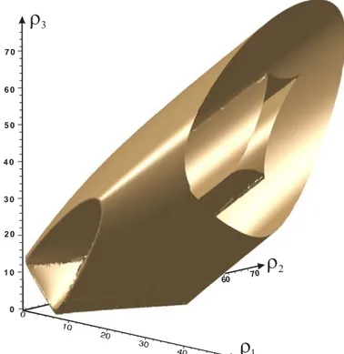
Figure 6 represents the singularities in the joint space of the manipulator studied when ρ1 varies from 0 to 50. To obtain this surface, we have imported the solutions obtained in step 4 into a CAD software, and we have meshed them together.
17
ρ
2ρ
1ρ
3 0 1 0 2 0 3 0 7 0 6 0 5 0 4 0 60 70Fig 6. Joint space singularity surfaces of the 3-RPR manipulator studied when ρ1 varies from 0 to 50.
The surface depicted in Figure 6 is of interest:
i. for planning trajectories in the joint space because it shows clearly the joint space regions that
are free of singularities.
ii. for manipulator design, because it offers a tool for defining the values of the joint limits such
that the joint space is a singularity-free box.
We can see clearly in figure 6 how the number of cusp points and the topology of the slices stabilize for ρ1>31.
This feature has been observed in many other manipulator geometries. For example, the 3-RPR manipulator defined by the following geometric parameters: A1= (0,0), A2= (3,0), A3 = (1.1,2.7), d1=
1.3, d2= 0.9 and d3 = 0.4 in an arbitrary length unit, has a constant pattern as soon as ρ1>5 (Fig. 7).
Note that, in contrast with the stabilized pattern obtained for the preceding manipulator, this pattern features a large void.
Most of the research work on parallel manipulators has focused on the analysis and optimization of the workspace. If the workspace is useful for manipulator design, the analysis of
18 singular curve patterns in the joint space can be used as a complementary tool to compare several manipulator geometries.
Fig 7. Stabilized singular curve patterns for another manipulator geometry plotted for ρ1=5 (left) and
ρ1=20 (right). 6. Conclusions
A procedure for computing joint space singularities of 3-RPR parallel manipulators has been presented in this paper. Then, the existence condition of cusp points defined by McAree9 has been reviewed and exploited. An algorithm able to detect and to compute cusp points inside any section of the joint space of any 3-RPR parallel manipulator has been established. To the best of the authors’ knowledge, such an algorithm had never been proposed before. The algorithm results in a 96th degree univariate polynomial that can be put in a factored form. We have showed with intensive numerical experiments that the coordinates of the cusp points are the real roots of a 24th degree univariate polynomial, which is one of the factors of the 96th polynomial. Finally, a descriptive
analysis of the singular curves in slices of the joint space of 3-RPR parallel manipulators has been conducted, with a special focus on the cusp points on these singular curves. It has been shown that, contrary to what arises in serial manipulators where any cross section of the workspace exhibits the same pattern of singular curves and cusp points, this pattern depends on the choice of the slice in the joint space for a given 3-RPR parallel manipulator. On the other hand, we have noticed that it is possible to have a constant pattern by adjusting the joint limits. It has been observed that the
19 maximum number of cusps depends on the manipulator geometry . No manipulators were found with more than eight cusp points. Most of the research work on parallel manipulators has been focused on the analysis and optimization of the workspace. This paper provides a complementary tool that helps better understand the topology of the joint space of parallel manipulators and finds applications in both design and trajectory planning.
7. References
1. J-P. Merlet, Parallel Robots, Kluwer Academics, 2000.
2. C. Gosselin, and J. Angeles, “Singularity analysis of closed loop kinematic chains,” IEEE
Transactions on Robotics and Automation, vol. 6, no. 3, 1990.
3. C. Gosselin, J. Sefrioui, and M.J. Richard, “Solution polynomiale au problème de la cinématique directe des manipulateurs parallèles plans à 3 degrés de liberté,” Mechanism and Machine
Theory, vol. 27, no. 2, pp. 107-119, 1992.
4. J. Sefrioui, and C. Gosselin, “On the quadratic nature of the singularity curves of planar three-degree-of-freedom parallel manipulators,” Mechanism and Machine Theory, vol. 30, no. 4, pp. 535-551, 1995.
5. P. Wenger, and D. Chablat, “Definition sets for the direct kinematics of parallel manipulators,”
8th Conference on Advanced Robotics, pp. 859-864, 1997.
6. I. Bonev, D. Zlatanov, and C. Gosselin, “Singularity Analysis of 3-DOF Planar Parallel Mechanisms via Screw Theory,” ASME Journal of Mechanical Design, vol. 125, no. 3, pp. 573– 581, 2003.
7. K.H. Hunt, and E.J.F. Primrose, “Assembly configurations of some In-parallel-actuated manipulators,” Mechanism and Machine Theory, vol. 28, no. 1, pp.31-42, 1993.
8. C. Innocenti, and V. Parenti-Castelli, “Singularity-free evolution from one configuration to another in serial and fully-parallel manipulators. Journal of Mechanical design. 120. 1998.
9. P.R. McAree, and R.W. Daniel, “An explanation of never-special assembly changing motions for 3-3 parallel manipulators,” The International Journal of Robotics Research, vol. 18, no. 6, pp. 556-574. 1999.
10. Xianwen Kong and Clément M. Gosselin, “Forward displacement analysis of third-class analytic 3-RPR planar parallel manipulators,” Mechanism and Machine Theory, Vol. 36, No. 9, pp. 1009--1018.
20 11. J. W. Burdick, “A Classification of 3R regional manipulator Singularities and Geometries,” In
Proceeding IEEE International Conference on Robotics and Automation, pp. 2670-2675,
Sacramento, California, 1991.
12. Ph. Wenger, “A New General Formalism for the Kinematic Analysis for all Non-Redundant Manipulators,” In Proceeding International Conference on Robotics and automation, pp. 442-447, Nice, France, 1992
13. J. El Omri and P. Wenger, “How to recognize simply a non-singular posture changing 3-DOF manipulator,” Proc. 7th Int. Conf. on Advanced Robotics, p. 215-222, 1995.
14. E. Ottaviano, M. Husty and M. Ceccarelli, “A cartesian representation for the boundary workspace of 3R manipulators,” In Proc. On Advances on Robots Kinematics, p. 247-254, 2004. 15. Ph. Wenger and D. Chablat, “Workspace and Assembly modes in Fully-Parallel Manipulators :
A Descriptive Study,” Advances in Robot Kinematics and Computational Geometry, Kluwer Academic Publishers, pp. 117-126, 1998.
16. M. Zein, Ph. Wenger and D. Chablat, “Singular curves and cusp points in the joint space of 3-RPR parallel manipulators”, Proceedings of the 2006 IEEE International Conference on
Robotics and Automation, Orlando, Florida, May 2006.
17. K. H. Hunt, “Geometry of Mechanisms,” Clarendon Press, Oxford, 1978.
18. B. Buchberger, G. E Collins and R. Loos: “Computer Algebra: Symbolic & Algebraic Computation,” Springer-Verlag, Wien, pp. 115-138, 1982.
19. M. Baili, P. Wenger and D. Chablat, “A classification of 3R orthogonal manipulators by the topology of their workspace,” IEEE Int. Conf. on Robotics and Automation, Louisiana, USA 2004.