HAL Id: hal-01421770
https://hal.archives-ouvertes.fr/hal-01421770
Submitted on 17 Mar 2020HAL is a multi-disciplinary open access archive for the deposit and dissemination of sci-entific research documents, whether they are
pub-L’archive ouverte pluridisciplinaire HAL, est destinée au dépôt et à la diffusion de documents scientifiques de niveau recherche, publiés ou non,
To cite this version:
Imed Zidane, Bogdan Marinescu, Mohamed Abbas-Turki. Linear time-varying control of the vibra-tions of flexible structures. IET Control Theory and Applicavibra-tions, Institution of Engineering and Technology, 2014, 8, pp.1760 - 1768. �10.1049/iet-cta.2013.1118�. �hal-01421770�
Linear Time-Varying Control of the Vibrations of
Flexible Structures
Imed Zidane, Bogdan Marinescu∗, Mohamed Abbas-Turki
SATIE, ENS Cachan & CNRS
61, Avenue du Président Wilson, 94235, Cachan Cedex zidaneimed@hotmail.com, bogdan.marinescu@satie.ens-cachan.fr,
abbas-turki@satie.ens-cachan.fr
Abstract
Recent results on pole placement for linear time-varying (LTV) systems are exploited here for the control of flexible structures. The infinite dimensional system is approached as usual by a restricted number of modes of interest, according to the frequency range in which the system is exploited. The dif-ference with the previous approaches (like, e.g., gain scheduling) is that only one finite dimension linear model is used and its parameters (frequency and damping of the modes) are varying according to the operating conditions. The control model is thus LTV and a regulator is analytically synthesized to en-sure closed-loop stability and performances. This regulator is also LTV and thus automatically (without any special switching action) tracks the operating
conditions of the system. The case of a flexible beam is studied in simulation as well as in laboratory experimentation. Hence, a suitable application of the proposed LTV synthesis is done to find a compromise between the complexity of interpolation and its efficiency. Furthermore, the bad dissipation factor of flexible systems leads them to be good candidates to proof the efficiency of the proposed gain scheduling strategy. This work validates on a real system the LTV pole placement approach and opens the way to a new gain scheduling strategy for the control of LTV, nonlinear or infinite dimensional systems. Key words: linear time-varying systems, flexible structures, vibrations at-tenuation
1 Introduction
Flexible structures are usually encountered in industry. A lot of studies have been thus devoted to the attenuation of their vibrations (see, e.g., [1] and [2]). The main difficulty comes from the infinite dimension of such systems ([3] and [4]). Indeed, it is reminded in Section 2 how the behavior of such a system is given by a class of oscillatory modes. For the control synthesis, a restricted number of modes is retained according to the frequency range in which the system is operated [5]. However, on the one hand, the charac-teristics (frequency and damping) of the members of this subclass of modes can vary in time [6]. On the other hand, the number of excited modes can change according to the operating band [7]. Adaptive and gain scheduling controls have been used to overcome these difficulties (see, e.g., [8]).
How-ever, in these approaches, it is difficult to guarantee the stability of the overall control scheme in case of hidden coupling modes (see, e.g., [9]). Moreover, according to [10], a low damping factor induces sensitivity in the model iden-tification. Indeed, due to a fast change in their phase inducing a low stability margin, flexible systems are very sensitive. For this reason, most of the pre-vious research related to flexible systems deal with their robustness and the most used criteria are H∞[11, 12, 13] and sliding mode [14]. Therefore, the
control performance of flexible systems is relegated to a less important target.
The knowledge of the different operating bands (cycle of operation of the machine, for example, the launch phase of a space launcher and other cycles) led us to use for the system a linear time-varying (LTV) model in order to capture the aforementioned variations of the system. The latter is still considered as infinite-dimensional described by a partial differential equation. As in the classic approaches, it is modeled by a restricted number of modes of interest but, in our approach, only one finite dimension linear model is used and its parameters (frequency and damping of the modes) are varying according to the operating conditions.
In [15] it has already been shown that necessary conditions for expo-nential stability can be provided if time-varying Lyapunov functions are used. Such stability conditions can be more directly obtained if the struc-ture (poles) of the LTV system is directly considered. More specifically, in [16] and [17] LTV notch filters have been used to damp vibrations of
flexi-ble structures and vehicles. They are placed on the control error path and their dynamics are tuned using the PD-eigenvalue theory introduced in [18] for differential operators with time-varying coefficients. The latter algebraic approach was extended and fully developed in [19] and related references to define poles and provide stability conditions for open as well as closed-loop LTV systems. In comparison to the PD eigenspectrum mentioned above, the poles are also defined for LTV systems given by differential operators which do not have roots over the field of definition of their coefficients. The field extensions needed in this case to find the poles allowed us to character-ize stability and to solve the pole placement problem for such general LTV systems. The output feedback pole placement method introduced in [20] is used here to analytically synthesize a regulator to directly ensure closed-loop stability and performances. This overcome the common difficulty to ensure the closed-loop stability when adapting the regulator to the evolution of the operating conditions. This latter difficulty is faced, for example, in the classical gain scheduling where several linear time-invariant (LTI) models are constructed around each operating point and an LTI regulator is syn-thesized for each model; the final regulator is obtained by switching among the members of the class of regulators according to the evolution of the op-erating conditions. The regulator which results from our approach is also LTV and thus automatically (without any special switching action) tracks the operating conditions of the system.
The paper is organized as follows. In Section 2, the standard modeliza-tion of flexible structures is briefly recalled. Secmodeliza-tion 3 gives the basics of the
LTV output feedback control. In Section 4 it is first shown how an LTV model for a smart beam can be obtained if some parameters are assumed varying with the operating conditions. The mathematical background pre-sented in Section 3 is used next for the synthesis of an LTV regulator which attenuates the vibrations of the beam. Section 5 presents simulation as well as laboratory results for the control of the smart beam while Section 6 is devoted to concluding remarks.
2 Flexible structures modeling
2.1 Dynamic equationsThe purpose of modeling is to know the resulting displacement field at any point of the structure. In the general case, the equations of the dynamics of the structure lead to partial differential equations (PDE), which do not admit simple analytical solutions, with the exception of the case of simple structures (for example, beams and plates simply supported on their contour). It is then necessary to perform a discretization of the problem where the deformation − →ω (x, y, z, t)∈ Rn is approached by − →ω (x, y, z, t) =!N i=1 − →ηi(x, y, z)qi(t), (1) where, (x, y, z) ∈ R3 are spatial coordinates, t is time variable, q
i ∈ R
are the general coordinates, −→ηi ∈ Rn the approximation functions and N
the number of degrees of freedom (DOF). For the beam, the −→ηi are given
by their proper modes, as shown in Fig 1. In our study, we used SDTools software to identify proper modes. In the case of the beam, these modes can
be found analytically [21]. Abscissa [m] Mo dal def ormations
Figure 1: Modal deformations of clamped-free beam: - Mode 1, - - Mode 2; · · · Mode 3; - . - Mode 4
The Lagrange formalism is used to provide the dynamic equations. Let T denote the kinetic energy and U the potential energy of the structure. Using the system description in equation (1), Lagrange equations can be written [1]: ∂ ∂t " ∂T ∂ ˙qi # −∂∂qT i +∂U ∂qi =Fi (2)
where Fi ∈ R are the generalized efforts on each DOF.
This leads straightforward to the following dynamic equation
M¨q + C ˙q + Kq = F (3)
where F = (F1,F2, . . . ,FN) is the vector of generalized efforts, M ∈
C ∈ Rn×n is the damping matrix. M is symmetric positive definite and K is symmetric semipositive definite. C is determined a posteriori because it is difficult to be modeled using structure characteristics.
We define the modal coordinates v ∈ Rn by projecting the generalized
displacement on the modal basis:
q(t) = Φv(t); ¨v(t) + Γ ˙v(t) + Ω2v(t) = ΦTF(t) (4) Φ∈ Rn×n is the modal basis matrix, Ω = diag{ω1, ..., ωN} is the modal
frequencies matrix. If we assume also that Γ = diag{2ω1ξ1, ..., 2ωNξN}
(Basile’s hypothesis [21]) which is generally verified in such systems [1], we get N independent equations of second order and every one defines a vibra-tion mode
¨
vi(t) + 2ξiωiv˙i(t) + ωi2vi(t) = ΦTFi(t) (5)
where ξi, ωi are, respectively, the damping and the frequency of the ith
vibration mode. Fi is the ith element of the vector F.
The parameter identification is done through the minimization of J which is the quadratic criterion of log modules:
J =$log|G(ω)| − log| ˆG(ω)|$2 (6)
where G and ˆGare respectively the transfer functions of the system and of the model and ω is the pulsation in rad/sec. Since the problem is non-convex, the proper pulsations are initialized visually for damping factors as well. Although the algorithm corrects sufficiently good pulsations, the very low value of the damping factor does not allow a good quality of its
identification even when using the log scale. As shown in the criterion, the most energizing modes are those selected by the model and they are at low frequencies. To minimize J, we use "fmincon" Matlab function on the frequency domain of interest. We point out that G does not vanish on the chosen set of frequencies.
2.2 State-space and transfer representations
The choice of the state vector
x = (ω1v1, ˙v1, ω2v2, ˙v2, . . . , ωNvN, ˙vN)T (7)
[22] leads to the following state-space representation ˙x(t) = Ax(t) + Bu(t) y(t) = Cx(t) + Du(t) (8) where A = diag{Ai}, Ai = 0 ωi −ωi −2ξiωi B = [0, b1, 0, b2, . . . , 0, bN]T C = [cp1, cv1, cp2, cv2, , . . . , cpN, cvN] (9)
bi and u (control input vector) depend on the type of the actuators used,
cpi, cvi and y depend on the sensors type (position or velocity sensors). D is
generally zero [21]. The choice (7) of the state vector gives the same range of values to its components which leads to a well conditioned problem.
The transfer function of a such structure is composed of the sum of the transfers of every subsystem. To simplify the exposal, consider a SISO
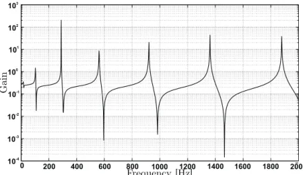
0 200 400 600 800 1000 1200 1400 1600 1800 2000 10-4 10-3 10-2 10-1 100 101 102 103 Gain Frequency [Hz]
Figure 2: Clamped-free beam modeling: input-output transfer. system. Its state representation (8) leads to the transfer function
H(s) = N ! i=1 ki s2+ 2ξ iωis + ωi2 (10) where N → +∞ and ki characterize the static gain of each mode.
The case of a clamped-free (cf. Fig. 4) beam was treated in this work. Its transfer is given in Fig. 2.
2.3 Flexible structure LTV model
For a control model, only a very restricted number of modes of a flexible structure model (10) must be considered. The most poorly damped modes in the frequency range in which the system is excited are usually chosen. However, the excitation usually varies with the operation conditions of the system, for example: aircraft taking off sequence. To capture this, a fixed control model (fixed number of modes) with time-varying characteristics (fre-quency and damping of the oscillatory modes) has been adopted in the se-quel. In this case, N in (10) is finite and ξi, ωi are time-varying. This
leads to an LTV transfer matrix. A specific formalism to handle this kind of mathematical objects is recalled in the next section.
3 LTV systems and control
3.1 LTV systems3.1.1 Linear systems as modules
In the algebraic framework initiated by Malgrange [23] and popularized in systems theory by several authors, a linear system is a finitely presented module M over the ring R = K[s] of differential operators in s = d/dt with coefficients in an ordinary differential field K. If K does not exclusively contains constants (i.e., elements of derivative zero), M is an LTV system.
R = K[s] is an Euclidean domain thus a two-sided Ore domain and it has a field of left fractions and a field of right fractions which coincide (see [24], [19]); this field is denoted by Q = K(s). A transfer matrix of an input-output LTV system (M, u, y) is a matrix with entries in Q [25]. The following notations are used in the sequel to denote matrices: H (or H(t)) is a matrix with entries in K, H(s) a matrix with entries in R (a polyno-mial matrix) and H(s) a matrix with entries in Q (a transfer matrix). The greatest common divisors lead to the following factorizations of a given LTV transfer matrix:
Proposition 1 [25]: Any LTV transfer matrix H(s) has:
(ii) right-coprime factorizations: H(s) = BR(s)AR(s)−1, i.e., y = BR(s)ξ
and u = AR(s)ξ
related by the diophantine equation1
AL(s)BR(s)− BL(s)AR(s) = 0. (11)
3.1.2 Autonomous systems
The autonomous part of the system corresponds to the torsion module T ∼= M/[u]R. The can be given by a state representation ˙x = Ax (where ˙x = dxdt), A∈ Kn×n or, equivalently, by a scalar differential equation
P (s)y = 0, P (s) = sn+ n−1 ! i=0 aisi (12) where y is a generator of T . 3.1.3 Stability of LTV systems
Let ∆K(α) ={αc = α + ˙cc−1, c∈ K, c '= 0} be the conjugacy class of α over
K. A skew polynomial has an infinite number of (right) roots. They belong to at most n conjugacy classes, where n is the degree of the polynomial [26]. A fundamental set of roots of a skew polynomial P (s) in (12) is a set {γ1, ..., γn} of n P-independent (in the sense of definition in [26]) roots. It is
directly linked to a fundamental set of solutions {y1, ..., yn} of the differential
equation (12) [27]: ˙yi/yi = γi, i = 1, ..., n. Notice that such a set may not
1When dealing with LTV systems, polynomials in (11) are skew, i.e., belongs to the
noncommutativeringR = K[s] equipped with the commutation rule sa = as+ ˙a, ∀a ∈ K,
exist over K, the initial field of definition of the coefficients of P (s), but over a field extension ˇK ⊃ K.
Definition 1: [19]
• A real analytic function f such that lim
t→+∞f (t) = +∞, ˙f (t) > 0,
lim
t→+∞
˙ f (t)
f (t) = 0 is called an Ore function. • If f is an Ore function, C(f) is an Ore field.
Definition 2 [27]: Let γi ∈ ˇK, i = 1, ..., n be a fundamental set of roots
of the polynomial P (s). If ˇKis an Ore field, the poles of T are the conjugacy classes {∆Kˇ(γi), i = 1, ..., n}. A set {γ1, ..., γn} of representatives of these
poles (i.e., γi∈ ∆Kˇ(γi)) is called fundamental if the γi’s are P -independent,
i.e., if they form a fundamental set of roots.
Theorem 1 [27]: Let {γ1, ..., γn} ∈ ˇK be a fundamental set of poles
of the autonomous system T . T is exponentially stable if and only if (iff) lim
t→+∞Re{γi(t)} < 0, i = 1, ..., n. )
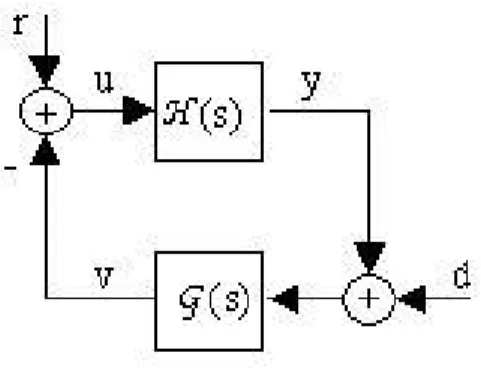
3.2 Closed-loop stability and pole placement
Proposition 2 [20]: It is assumed that the plant of the classical closed-loop in Fig. 3 is controllable and observable, i.e., completely described by its transfer matrix H(s). Consider factorizations (i) and (ii) for the plant Qp×m * H(s) = A
L(s)−1BL(s) = BR(s)AR(s)−1 and for the regulator
G(s) = SL(s)−1RL(s) = RR(s)SR(s)−1. Then:
1. Polynomials
and
Acl(s) = SL(s)AR(s) + RL(s)BR(s) (14)
have the same conjugacy classes of roots.
2. If the roots of Acl(s)(or, equivalently, of Acl(s)) belong to an Ore field,
then the poles of the closed-loop system are the conjugacy classes of a fundamental set of roots of Acl(s) (or Acl(s)).
3. If G(s) is chosen such that the poles of the closed-loop system satisfy the condition of Theorem 1, then the control-loop system is internally exponentially stable, i.e., all transfers r +→ y, r +→ v, d +→ y and d +→ v in Fig. 3 are exponentially stable. )
The output-feedback pole placement problem consists thus in solving the Bézout equation (13) (or, equivalently, (14)) for SR(s) and RR(s) (or,
equivalently, for SL(s)and RL(s)).
4 The vibrations control of a smart beam
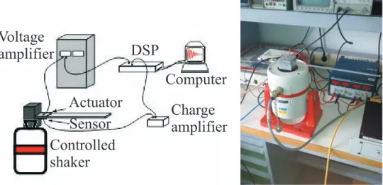
4.1 Description of the systemThe structure studied is an aluminum beam clamped-free, of which charac-teristics are given in Table 1. The experimental control-loop is presented in Fig.4. It is equipped with a piezoelectric actuator and sensor, glued on each side of the beam, at the clamped side. The beam is fixed on a shaker which generate vibrations. This flexible structure has its modes at low fre-quency (16Hz for the first mode), the same frefre-quency range as the aviation structures. The input and output signals are the voltages measured by the sensor and, respectively, applied to the actuator. The sensor is connected to a charge amplifier. The aim of this amplifier is to apply, via the opera-tional amplifier, a zero potential difference between the two electrodes of the sensor, in order to cancel the influence of capacity (wiring or sensor). The control law is computed and applied via a dSpaceT M card DS1103. For a
significant deformation of the beam, the voltage amplifier is used with gain of 13. The magnitude of the Bode plot of the transfer function between the above input and output is given in Fig.2. A photo of the experiment set-up is given in Fig. 4.
Length Width Thikness Material Young module Density
30 cm 1 cm 1.56 mm AU4G 78 GPa 2970 kg.m−3
Table 1: beam cracteristics.
The following scenario is considered to reproduce the control problem with this benchmark. Assume that the shaker excites the beam with a
Computer
DSP
Voltage
amplifier
Actuator
Sensor
Controlled
shaker
Charge
amplifier
Figure 4: Experimental control-loop
sinusoidal signal γ(t) = sin(2πf(t).t) which frequency profile is known. For our structure, the following frequency function was chosen:
f (t) = 1 + 120t
1 + t . (15)
This frequency profile excites the first two modes (at f1 = 16Hz and
f2= 100Hz) and captures the variation of the excitation band.
Parameter k1 ξ1 ω1 k2 ξ2 ω2
Value 2500 0.01 104 rad/s 105 0.5+0.01t
1+t 600 rad/s
Table 2: LTV model parameters.
To attenuate the vibrations of the structure, the classic LTI solution, called Positive Position Feedback (PPF) controller [2], consists in taking the two modes into consideration for the controller design whatever the frequency profile of the exciting signal is. As a result, even if stability is ensured, performances are low. An LTV model is used to improve these results.
4.2 LTV model of the beam
A second order LTV model of type (16) for which the most energetic modes have been considered is used for the beam:
H(s) = Pk1 1(s) + k2 P2(s) (16) where P1(s) = s2+ 2ξ1ω1s + ω12 P2(s) = s2+ . 2ξ2ω2+ ˙ ξ2ξ2 1−ξ2 2 / s +.ω2 2− ˙ ξ2ω2 1−ξ2 2 / (17)
and the expression of P2(s)is such that H(s) has the following fondamental
set of poles: λ1,2 =−ξ1ω1± jω1 0 1− ξ2 1 λ3,4 =−ξ2(t)ω2± jω2 0 1− ξ2(t)2. (18) ξ2(t) is chosen to have the same dynamic as the frequency profile as
shown in Table 2 along with the other parameters of the model. It ranges from 0.5 at the begining -to model the absence of excitation of the second mode to 0.01 when the second mode is excited. In order not to change the phase of the first mode, ξ2(t)does not start at 1.
4.3 LTV controller design
To design the controller, a left-coprime factorization (i) is written for (16)
where AL(s) is the (left) minimal polynomial of P1(s) and P2(s) (see,
e.g., [19]):
AL(s) = (P1(s), P2(s))l; BL(s) = k1B1(s) + k2B2(s) (20)
B1(s), B2(s) are such that AL(s) = B1(s)P1(s) = B2(s)P2(s).
As the damping of the modes characterize the amplitude of the vibra-tions of the structure, the purpose of the active control of vibravibra-tions is to assign desired values ξi to the dampings. The control system in Fig. 4 leads
to the closed loop in Fig. 3, where:
• the reference signal r = 0;
• the disturbance signal d represents the contribution of the shaker in the sensor output signal;
• the control signal u = −v calculated by the controller gives an output y that "ideally" neutralize the shaker effect.
The controller is synthesized using the procedure described in Section 3 to reach the following objectives:
• Ensure the stability of the closed-loop system;
• Increase the damping of the two modes: ¯ξ1= ¯ξ2= 0.3;
• Keep the same natural frequencies; • Ensure the causality of the controller;
• Do not excite the neglected modes.
For this, the poles of the closed-loop system are placed to: λ1,2=−ξ1ω1± jω1 1 1− ξ21 λ3,4 =−ξ2ω2± jω2 1 1− ξ22. (21) As a consequence, Acl is chosen to be:
Acl(s) = (s2+ 2¯ξ1ω1s + ω12)(s2+ 2¯ξ2ω2s + ω22)Q(s) (22)
where Q(s) represents additional exponentially stable poles to ensure the causality of the controller and not affect the remaining modes. Giving the forms of H(s) and Acl(s), the factors SR(s)and RR(s)of the controller G(s)
in equation (13) must have the following form: SR(s) = s3+ s2(t)s2+ s1(t)s + s0(t) RR(s) = r3(t)s3+ r2(t)s2+ r1(t)s + r0(t) (23) Moreover, in order to ensure causal solutions G(s) in (13),
Q(s) = (s + 150)(s + 200)(s + 300). (24)
4.4 LTV controller computation and implementation
Next, the controller coefficients in (23) must be found by solving the Bézout equation (13) by identifying the coefficients of the two terms.
The computation of SR(s)and RR(s)is done using a symbolic
computa-tion tool. As the obtained coefficients of the two polynomials were too com-plicated, we proceeded to their first order Padé-type simplification in order to be easily used in simulations and real-time tests (Table III in Appendix).
First, notice that the obtained simplified expressions of the coefficients pro-vide trajectories close the ones of the exacte expressions as shown in Fig. 12 of Appendix.
Next, the simplified controller provides a closed-loop dynamic very close to the desired one. Fig. 5 shows that the closed-loop poles obtained using the simplified controller are quite close to the desired poles. Notice that this kind of simplification can be carried out also when working with large systems (polynomial ALof higher degree) and leads to simple expressions of
the coefficients of the regulator (as the ones in Table III of Appendix) which can be easily implemented to obtain a higher order regulator. This opens the way to applications which need regulators of higher order.
Figure 5: Closed-loop poles.(+ : desired poles, o : variation in time of the poles obtained with the simplified controller).
To provide a causal implementation of the regulator, one canonical LTV state-space form is computed from the factors (2) [27]. In our case the right-form is :
Actrl = 0 1 0 0 0 1 −s0(t) −s1(t) −s2(t) , Bctrl= 0 0 1 Cctrl = 2 r0(t)− r3(t)s0(t) r1(t)− r3(t)s1(t) r2(t)− r3(t)s2(t) 3 (25)
5 Control results
The designed LTV controller was both tested in simulation and on the real system.
5.1 Simulation results
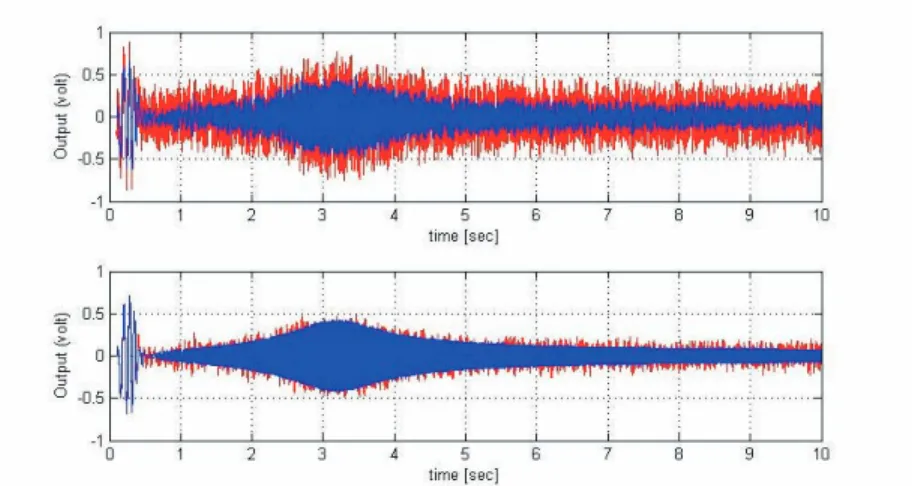
The simulation results in Fig. 6 (a)-(b) show that the controller damps the two vibration modes at the level expected from the design. It has also been studied the effect of actuator saturation: when this is taken into account (Fig. 6 (a)), the damping action is less efficient. Robustness against high order dynamics has also been tested by injecting a white noise of frequency 150Hz on the measurement y. Fig. 7 shows that this noise is correctly filtered (at least not amplified) by the closed-loop.
5.2 Experimental results
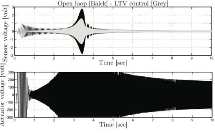
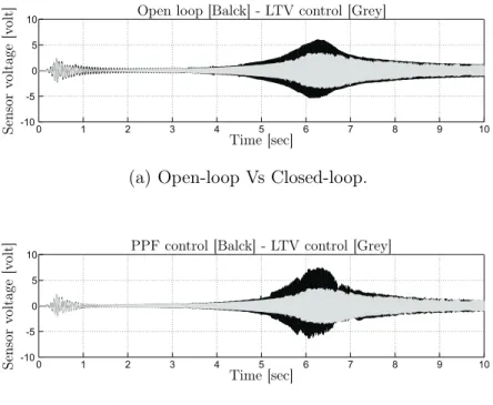
Four comparisons were performed on the experimental benchmark presented in Section 4 (for which the saturation of the actuator cannot be avoided):
• the open-loop compared with the LTV closed-loop to illustrate the effect of such an active control (Fig. 8 (a));
0 1 2 3 4 5 6 7 8 9 10 -3 -2 -1 0 1 2 3 0 1 2 3 4 5 6 7 8 9 10 -300 -200 -100 0 100 200 300 Sens or voltage [v olt] Time [sec] Time [sec] Ac tu at or vo lt ag e [v ol t]
Open loop [Balck] - LTV control [Grey]
(a) Control with saturation.
0 1 2 3 4 5 6 7 8 9 10 -3 -2 -1 0 1 2 3 0 1 2 3 4 5 6 7 8 9 10 -1500 -1000 -500 0 500 1000 1500 Sens or voltage [v olt] Time [sec] Time [sec] Ac tu at or vo lt ag e [v ol t]
Open loop [Balck] - LTV control [Grey]
(b) Control without saturation.
Figure 6: Simulation results: Control with and without saturation. • the proposed LTV controller compared with the classic (PPF) LTI
controller (Fig. 8 (b));
• the proposed LTV controller compared with the two LTI controllers designed from its parameters frozen for t → 0 and t → +∞ (Fig. 9 (a) and (b)).
Figure 7: Simulation results: robustness test (Up: Output and Noised Out-put; Down: Output with noised feedback and Output without noised feed-back).
Fig. 8 (a) shows that the control system ensures stability and good damp-ing of the vibrations. However, we notice that the second mode is more damped than the first one. This is mainly due to physical constraints inher-ent to the system (independinher-ent of the controller used). Indeed, the static gains k1 and k2 reported in Table. 2 show that the actuator has more effect
on the second mode than the first one. This makes the control of the first mode difficult, knowing the limitation of the actuator in practice. Of course, this is not the case in simulation with no actuator constraints as shown in the above section.
Fig. 8 (b) illustrates the advantage of the LTV controller over a conven-tional controller. Both techniques have similar effects on the first mode, but the PPF control amplifies the second mode instead of damping it. This is quite logical, because the PPF control was designed to control only the first
0 1 2 3 4 5 6 7 8 9 10 -10 -5 0 5 10 Sens or voltage [v olt] Time [sec]
Open loop [Balck] - LTV control [Grey]
(a) Open-loop Vs Closed-loop.
0 1 2 3 4 5 6 7 8 9 10 -10 -5 0 5 10 Sens or voltage [v olt] Time [sec]
PPF control [Balck] - LTV control [Grey]
(b) LTV controller Vs PPF controller.
Figure 8: Experimental results: Comparaison LTV controller Vs Open-loop and PPF controller.
mode, so the second one it is not considered during the design.
Fig. 9 (a) and (b) put into evidence the advantage of variation of the parameters of the LTV controller to continuously adapt to the disturbance. The same figures show that the first LTI controller mitigate well the first mode, but deteriorates progressively when the damping of the second one is decreasing. The second LTI controller does the opposite. The LTV controller combines the two advantages and ensures stability in a simple and direct way. Notice also that, in order to control the two modes with a classic control (like LQG, H∞), the resulting controller must be at least of order 4 to have
the same performance as our LTV controller of order 3. Notice also that the good results obtained in experimentation prove, in addition to performances,
0 1 2 3 4 5 6 7 8 9 10 -10 -5 0 5 10 Sens or voltage [v olt] Time [sec]
LTI control [Balck] - LTV control [Grey]
(a) LTV controller Vs LTI controller (LTV at t → 0).
0 1 2 3 4 5 6 7 8 9 10 -4 -2 0 2 4 Sens or voltage [v olt] Time [sec]
LTI control [Balck] - LTV control [Grey]
(b) LTV controller Vs LTI controller (LTV at t → ∞).
Figure 9: Experimental results: Comparaison LTV controller Vs LTI con-trollers (LTV at t → 0) and (LTV at t → ∞).
robustness against unmodeled dynamics. Indeed, on the one hand, the reg-ulator is synthesized for only 2 modes of the system and, on the other hand, it is used on the real physical in its simplified form presented in Section 4.4 and Appendix.
6 Conclusions
This work validates on a real physical system the LTV pole placement ap-proach [20]. Moreover, hints for the practical implementation like, e.g., the regulator truncation, have been proposed. This opens the way to industrial applications for which the LTV modelization and control were long time avoided because both of the lack of theoretical results and the complexity of
solutions and computations when such results exist.
This LTV approach opens also the way to a new scheduling technique. Indeed, large operating domains can be covered with an LTV model for which some parameters are varied. This stands both for nonlinear systems (for which the linearization around given trajectories give LTV models) and for infinite dimensional ones as for the case treated here. As for this approach stability is directly ensured, the forthcoming effort will be concentrated on the way to choose/construct the scheduling variables in order to optimally capture the variations of the operating conditions.
The case of flexible structures will be further investigated by considering higher order systems like the multidimensional structures, e.g., vibrating plates.
References
[1] Gerardin, M. and Rixen, G.: ’Théorie des vibrations, application la dynamique des structures’, Masson, Physique fondamentale appliquée, 2nd edn. 1996.
[2] Preumont, A.: ’Vibration control of active structures: An introduction’, Springer-Verlag, Solid Mechanics and its Applications, 179, 1997, 3rd edn. 2011.
[3] Lasiecka, I.: ’Galerkin approximations of infinite-dimensional compen-sators for flexible structures with unbounded control action’, Acta Ap-plicandae Mathematica, 1992, (28), pp. 101-133.
[4] Luo, Z. H., Guo, B. Z. and Morgül, Ö.: ’Stability and stabilization of infinite dimensional systems with applications’, Springer-Verlag, 1999. [5] Schilders, W. H. A., Van der Vost, H. A. and Rommes, J.: ’Model
order reduction: Theory, research aspects and applications’, Springer-Verlag, 2008.
[6] Jeanneau, M., Alazard, D. and Mouyon, P.: ’A semi-adaptive frequency control law for flexible structures’. Proc. of the American Control Con-ference (ACC), Portland, USA, 1999.
[7] Mohammadpour, J. and Scherer, C. W.: ’Control of Linear Parameter Varying Systems with Applications’, Springer-Verlag, 2012.
[8] Shojaei, K. and Shahri, A.M.: ’Adaptive robust time-varying control of uncertain non-holonomic robotic systems’, IET Control Theory and Applications, 2012, 6, Iss. 1, pp. 90-102.
[9] Leith, D.J. and Leithead, W.E.: ’Input-output linearization velocity-based gain scheduling’, Int. J. of Contr., 1999, Vol. 72, 1999, pp. 229-246. [10] Bérard, C. and Puyou, G.: ’Gain scheduled flight control law for a flexible aircraft : A practical approach’, Automatic control in Aerospace, 25-29 June 2007, Toulouse, France.
[11] Balas, G. J. and Doyle, J. C.: ’Robustness and Performance Tradeoff s in Control Design for Flexible structures’, IEEE Transactions on Control Systems Technology, 1994, 2(4), pp.352-361.
[12] Halim, D. and Reza Moheiani, G. De M.: ’Experimental Imple-mentation of Spatial H∞ Control on a Piezoelectric-Laminate Beam’,
IEEE/ASME Transactions on Mechatronics, 2002, 7(3), pp. 346-356. [13] Cavallo, A., D Maria, G. and Pirozzi, S.: ’Robust Control of Flexible
Structures With Stable Bandpass Controllers’, Automatica, 2007, 44, pp. 1251-1260.
[14] Gu, H. and Song, G.: ’Active Vibration Supression of a Flexible Beam with Piezoceramic Patches using Robust Model Reference Control’, Journal of Smart Materials and Structures, 2007, 16(4), pp. 1453-1459. [15] Gielen, R.H. and Lazar, M.: ’Stabilisation of linear delay difference inclusions via time-varying control Lyapunov functions’, IET Control Theory and Applications, 2012, 6, Iss. 12, pp. 1958-1964.
[16] Adami, T., Sabala, R. and Zhu, J. J.: ’Time-varying notch filters for control of flexible structures and vehicles’. Proc. of the 22nd Digital Avionics Systems Conference, Indianapolis, Indiana, Oct. 2003.
[17] Adami, T. and Zhu, J. J.: ’Control of a flexible, hypersonic scramjet vehicle using a differential algebraic approach’. Proc. AIAA Guidance, Navigation and Control Conference, Honolulu, HI, August, 2008. [18] Zhu J. J.: ’Series and parallel d-spectra for multi-input-multi-output
linear time-varying systems’, Proc. of the South-Eastern Symposium on Systems Theory, Baton Rouge (LA-US), 1996, pp. 125-129.
[19] Bourlès, H. and Marinescu, B.: ’Linear Time-Varying Systems, Algebraic-Analytic Approach’, LNCIS Springer-Verlag, 2011.
[20] Marinescu, B.: ’Output feedback pole placement for linear time-varying systems with application to the control of nonlinear systems’, Automat-ica, (46), No. 4, 2010, pp. 1524-1530.
[21] Leleu, S.: ’Amortissement actif des vibrations d’une structure flexible de type plaque à l’aide de transducteurs piézoélectriques’. PhD thesis, Ecole Normale Supérieure, Cachan, France, 2002.
[22] Hac, A. and Lui, L.: ’Sensor and actuator location in motion control of flexible structures’, Journal of sound and vibration, 1990, 167, (2), pp. 239-261.
[23] Malgrange, B.: ’Systèmes différentiels à coefficients constants’. Sémi-naire Bourbaki, 246, 1962-1963, pp. 1-11.
[24] Cohn, P. M.: ’Free rings and their relations’, Academic Press, London Mathematical Society Monograph, No. 19, 2nd edn. 1985.
[25] Fliess, M.: ’Une interprétation algébrique de la transformation de Laplace et des matrices de transfert’, Linear Algebra and its Appli-cations, 1990, (203), pp. 429-443.
[26] Lam, T. Y. and Leroy, A.: ’Wedderburn polynomials over division rings, I’, Journal of Pure and Applied Algebra, 2004, 186, pp. 43-76.
[27] Marinescu, B. and Bourlès, H.: ’An intrinsic algebraic setting for poles and zeros of linear time-varying systems’, Systems and Control Letters, 2009, 58, pp. 248-253.