Chord Length Distribution: relationship between Distribution Moments and Minkowski Functionals

HAL Id: hal-01637703

https://hal.archives-ouvertes.fr/hal-01637703

Chord Length Distribution: relationship between

Distribution Moments and Minkowski Functionals

Frédéric Gruy

To cite this version:

Frédéric Gruy. Chord Length Distribution: relationship between Distribution Moments and Minkowski Functionals . 2017. �hal-01637703�

Chord Length Distribution: relationship between

Distribution Moments and Minkowski Functionals

Frédéric Gruy

Ecole Nationale Supérieure des Mines, 158 Cours Fauriel, 42023, Saint-Etienne, France [email protected]

Phone: 0033477420202 Corresponding author

Keywords: Chord Length Distribution, Minkowski’s functionals, Integral Geometry, Monte Carlo Simulation, Electromagnetic Wave Scattering

Abstract: the chord length distribution (CLD) and its nth moments (n≤4 ) have been calculated for a set of 3D-convex bodies. From these data, an empirical relation between the CLD moments and the Minkowski functionals is proposed for the second and third order CLD moments based on the Cauchy formula initially established for the first and fourth order moments in three-dimensional space. The approximation is improved by considering an additional parameter as the number of body vertices. Moreover it is shown that the data set and the empirical expression respect the inclusion inequalities recently found by L. Heinrich (Applied Mathematical Sciences, 8(2014)8257-8269).

1. Introduction

Chord Length Distribution appears in the modelling of the interaction between electromagnetic waves and matter. Applications can be found in the field of radiology, dosimetry [1] and particle sizing [2-3]. Analytical calculations of CLD have been achieved for numerous 2D and 3D particle shapes by different investigators: disc, triangle, rectangle, regular polygon [4,5], sphere, hemisphere [6], cylinders of various cross sections [7-8], spheroids [9], polyhedron [10-11].

CLD have been intensively studied by researchers in the field of the small angle scattering using X-rays (SAXS) [2]. Therefore we may compile the main results of the literature especially these ones concerning the SAXS theory. From these data, common characteristics of CLD may emerge. Moreover, additional properties have been discovered by the mathematicians. In the following, the CLD will be denoted D l where l is the chord length. _l( )

We may consider the CLD of any convex body as the CLD of an equivalent spheroid or ellipsoid, i.e. a body with a smooth shape, modified by specific geometrical features. The latter ones are important for the shape of the CLD curve. They consist in flat faces as crystal facets, parallel (flat or curved) surfaces, parallel tangent planes, edges and corners. They correspond to discontinuities of the distribution density or its derivative.

the other for l=2b, a and b being the semi-axes. A discontinuity of dD ll( ) /dl will occur at

these values. Wu and Schmidt [14] have investigated the properties of D l when the chord _l( )

is in the neighbourhood of an extremal chord. They give expressions for D l around the _l( )

extremal chord values denoted L. They show that D l is continuous for l=L whereas l( )

( ) / l

dD l dl is not. Ciccariello [15-17] generalized the work of Wu and Schmidt: he considers

the property of parallelism between some parts of body boundaries. He studied the case where the locus of the extremal chord ends is a surface. For instance, this surface is a sphere for

l=2R if the particle is a sphere with radius R. One can show that D l becomes discontinuous _l( )

for this chord length value. If the parallelism occurs between two partial surfaces of the body, a discontinuity of D l occurs at l=L, L being the distance between the two parallel surfaces. _l( )

The contribution of the parallelism to D l for ll( ) →L is given by Ciccariello. The presence of edges leads to additional terms for D l at l=0. Ciccariello et al. [16, 19] and Sobry et al. l( )

[18, 20] have shown that D_l

( )

0 is a simple function of the dihedral angle and of the edge length. All the edges contribute to Dl

( )

0 . Edges (and corners) also contribute to dD ll( ) /dl_l=0 [21]. However, it seems difficult to systemize this contribution.

These features may constitute a rule set for building an approximate CLD of a given convex body [22]. It results that the variation of the chord length density against the chord length may be very non monotonic. At the same time, some of the previous authors have calculated the moments of such CLD (see for instance [1] for spheroids). General formula, called Cauchy formula, had been previously established by mathematicians [23]. They concern the first and the fourth CLD moments in the case of 3D body. These are expressed as a function of the volume and the surface area of the body. However there exists no such formula for the second and the third CLD moments. Whereas CLD is a characteristic of the body under the stochastic geometry, first and fourth moments are a function of quantities

issued from integral geometry [24]. So, surface area and volume are the simplest components of a parameter set known as scalar Minkowski functionals (MF). The latter constitute a complete set of descriptors as shown by Hadwiger [25]: any valuation of a convex body respecting certain mathematical properties, i.e. additivity, translation and rotation invariance, continuity, is a linear combination of the MF’s. In 3D space, the four scalar Minkowski functionals are proportional to the surface area, the volume and the mean and Gaussian curvatures [26, 27]. It is clear that the CLD’s, and then their moments, do not

respect the additivity property that would

be: D Kl

[

1∪K2

]

=D Kl

[ ]

1 +D Kl

[ ]

2 −D Kl

[

1∩K2

]

. As a consequence, CLD moments cannot be written as a linear combination of MF’s.

Voss and Cruz-Orive [28] have studied the second moment of the random measure of the intersection between a compact set and a geometric probe, e.g. point, line or line segment. More specifically, they propose an analytical expression between the second moment of CLD and the geometric covariogram of the body. Heinrich [29-31] has considered the second-order moments of CLD for various bodies in any space dimension. He was precisely interested in searching lower and higher bounds, i.e. inclusion inequalities, for CLD moments. The so determined bounds are function of the volume, surface area and mean curvature of the body [31].

The aim of this paper is to examine the relation between CLD moments and scalar Minkowski’s functionals. This problem will be tackled from the point of view of

The paper is organized as follows: section 2 specifies the selected body classes, the methods used for calculating CLD moments and MF’s, the generated data set. Section 3 analyses the data and builds step by step the approximate expression linking CLD moments and MF’s. Section 4 concludes the paper.

2. Tools and methods for data generation

Several shape sets have been considered: sphere (radius R), cylinders (base radius R, height H), ellipsoids (semi-axes A, B, C), parallelepipeds (edge lengths A, B, C), triangular pyramids (edge length A, height H) triangular bipyramids (edge length A, height H), triangular prism (edge length A, height H), octahedron. All these bodies are convex; certain (sphere, ellipsoids) are smooth whereas the others are facetted and have linear or circular edges and corners. The aspect ratio is within the [0.05; 1] range. The CLD moments and the Minkowski functionals of these bodies have been calculated by the procedures described in sub-sections 2.1 and 2.2.

2.1. Calculation of the CLD moments

Our work focuses on CLD calculations with 3D uniform flow of lines.

Throughout the paper and the literature, the chord length distribution (density) is written

( )

l

D l where 0≤ ≤l lmax. D l dll

( )

is the number of chords within the l-range

[

l l, +dl

]

. D ll

( )

is usually presented as normalized, i.e

( )

max 0 1 l l D l dl =

∫

.

A software based on a Monte Carlo algorithm was employed to generate an isotropic uniform random line across the geometric object, and to collect the chord length segments. The same framework for the Monte Carlo Simulations (MCS) of the different particle shapes has been used.

Consider a sphere with radius RMC larger than lmax/2 and its centre located at the origin of the

coordinate system. The body is located inside this sphere and its centre of mass matches the origin. The way used to define the random straight line is the following: A direction and a point belonging to the plane orthogonal to that direction and tangent to the sphere are considered. The coordinate system of the plane is composed of the point of tangency and the vectors from the usual spherical coordinate system. The line will be defined by the two angles, polar

θ

and azimuthal

φ

, and the two coordinates xP, yP of the point in the plane. Four random

numbers [32] are chosen for the values of the variables cos

θ

,

φ

, xP and yP. The line intersects

the sphere at two points denoted M1 and M2. This algorithm is known to provide a translation

and rotation invariant density [33].

Depending on the body, the straight line between M1 and M2 may intersect the particle 0 or 2

times. The intersection points will be analytically determined and the corresponding distances calculated.

The MC sampling distribution may be visually represented as a discrete probability histogram. The chord length between zero and the maximal possible length, i.e. 2RMC, is divided on

m-bins with the equal size of ∆l. The value of m is has been taken to 400. All simulation runs

have been carried out by generating 108 unbiased random lines. Only a smaller number Nl

lines cross the body. The sampling error is smaller than 10-4. As already mentioned, the CLD is usually presented as normalized:

( )

/

(

)

l i i

2.2. Calculation of the Minkowski functionals

We consider in this paper convex bodies. Integral geometry introduces scalar Minkowski Functionals (MF) as shape measures. The body K is a compact set bounded by a surface ∂K. The four Minkowski functionals are defined by:

( )

0 V W K = =V

∫

dV (1)

( )

1 1 3 _K 3 S W K dA ∂ =

_∫

= (2)

( )

2 2 1 3 _K W K G dA ∂ =

_∫

(3)

( )

3 3 1 3 _K W K G dA ∂ =

_∫

(4)

V and S are the volume and the surface area of the body. The mean and Gaussian curvatures

on ∂K are G2 and G3, respectively. They obey the relations:

(

)

2 1 2 / 2

G = k +k (5)

3 1 2

G =k k (6)

k1 and k2 are the principal curvatures on ∂K. The previous relations can be straightforwardly

applied for smooth bodies. If the body has edges or corners, the MFs are calculated from the Steiner’s formula [26] that relies the volume of the dilated body K⊗B_εto the dilation factor ε

by means of a polynomial:

(

)

( )

( )

( )

2

( )

3

0 0 3 1 3 2 3

W K⊗B_ε =W K + W K

ε

+ W K

ε

+W K

ε

(7)

B_ε is a ball with radius

ε

.

For each selected body, one calculates the area, the volume, the W2 and W3 values, the CLD

moments of order 1, 2, 3 and 4. So, we have for W2:

2 4 3 W = π R for sphere (8)

(

)

2 3 W =π H+πR for cylinder (9)

(

)

2 3 W =π A+ +B C for parallelepiped (10)

For ellipsoids, W1 and W2 can be obtained from data compiled by Wolfram [34] and Rivin

[35].

For polytopes, a dedicated software based on equation (7) has been used for calculating W0,

W1 and W2.

As we are only dealing with bodies with convex hull and no holes, W3 is equal to

4 / 3π following the Gauss-Bonnet theorem. Therefore W3 is not a relevant parameter for the

shape set studied herein.

2.3 Data set

The table 1 contains the raw data after applying the methods depicted in subsections 2.1 and 2.2. The geometrical parameters of the bodies are dimensionless. The maximum length lmax of

the bodies is smaller than 4. The radius RMC of the sphere enclosing the body is therefore

taken equal to 2. As the CLD is defined as normalized, the moment with null order M0 is

N shape Geometrical characteristics S=3W1 V=W0 W2 M1 M2 M3 M4 1 sphere R=1 12.57 4.189 4.189 1.333 2 3.2 5.332 2 cylinder R=1 H=1 12.57 3.1416 4.337 1 1.294 1.893 2.994 3 cylinder R=1 H=2 18.85 6.283 5.384 1.334 2.236 4.119 8.003 4 cylinder R=0.5 H=2 7.854 1.571 3.739 .8 .8019 .924 1.2 5 cylinder R=0.2 H=2 2.765 0.2513 2.752 .3638 .1682 .102 .0873 6 cylinder R=1 H=0.1 6.911 0.3142 3.395 .1818 .0605 .0444 .0542 7 spheroid A=2 B=1 C=1 21.48 8.377 5.788 1.561 2.831 5.696 12.48 8 spheroid A=1 B=2 C=2 34.69 16.75 7.165 1.933 4.410 11.22 30.95 9 spheroid A=2 B=0.2 C=0.2 3.966 0.335 4.32 .3383 .15 .0975 .1076 10 spheroid A=2 B=2 C=0.2 25.89 3.351 6.617 .5181 .4676 .7358 1.661 11 Parallelepiped A=1 B=1 C=1 6 1 3.1416 .6663 .5972 .5985 .6358 12 parallelepiped A=2 B=1 C=1 10 2 4.189 .8009 .8712 1.097 1.533 13 parallelepiped A=2 B=2 C=0.5 12 2 4.712 .6663 .6423 .8162 1.2738 14 parallelepiped A=2 B=1 C=0.5 7 1 3.665 .5716 .4568 .4552 .5461 15 parallelepiped A=3 B=0.3 C=0.3 3.78 0.27 3.770 .2856 .1162 .07 .0735

16 octahedron Regular A=1 3.464 0.4714 2.4619 .5443 .3825 .2976 .245 Table 1: Minkowski functionals and CLD moments of various bodies.

N shape Geometrical Characteristics

S=3W1 V=W0 W2 M1 M2 M3 M4

17 Tetrahedron Regular A=1 1.732 0.118 1.911 .2722 .1117 .0553 .0306 18 T-pyramid A=1 H=3 4.9538 0.433 4.008 .3495 .1966 .1482 .1448 19 T-pyramid A=2 H=2/3 4.3778 0.3849 3.2362 .3517 .2005 .1477 .1293 20 T-prism A=1 H=1 3.866 0.433 2.618 .4481 .2904 .2213 .1854 21 T-prism A=1 H=3 9.866 1.299 4.7124 .5266 .4217 .4540 .6531 22 T-prism A=2 H=0.3 5.2641 0.5196 3.4558 .3949 .2318 .1875 .1959 23 T-prism A=1/4 H=3 2.3041 0.0812 3.5343 .141 .0317 .0124 .0113 24 T-bipyramid A=1 H=1.633 2.5981 0.2357 2.2505 .3629 .1910 .1187 .0817 25 T-bipyramid A=2 H=0.3266 3.6 0.1886 3.1453 .2095 .0820 .0482 .0376 26 T-bipyramid A=1/4 H=3.266 1.2259 0.0295 3.439 .0962 .0164 .0049 .0029 27 T-bipyramid A=1/4 H=2.041 0.7674 0.0184 2.1676 .0961 .0159 .0041 .0017 28 T-bipyramid A=3 H=0.245 7.8718 0.3182 4.7131 0.1617 .0607 .0442 .0492

3. Analysis and discussion 3.1 Introduction

The mean chord length of a convex body is related to V and S by means of the first Cauchy formula: 1 0 4 / M l V S M = = (11)

The second Cauchy formula refers to the 4th moment: 2 4 4 0 12 M V l M π S = = (12)

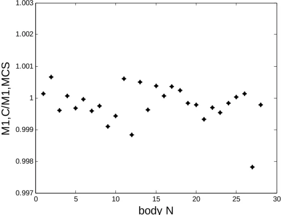
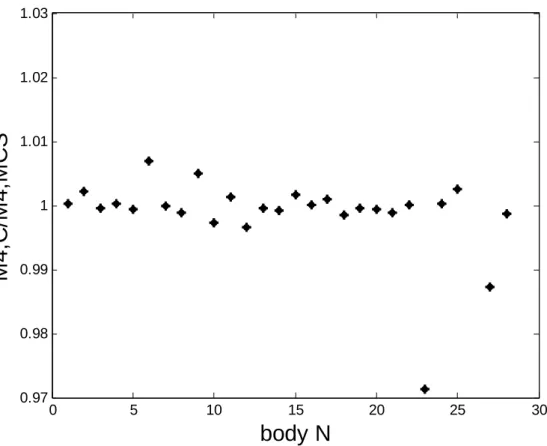
The figure 1 presents the comparison between the Cauchy l value (Eq.11) and the MCS l value for the first order moment. This has been performed for the 28 selected bodies. The deviation is smaller than 10-3 except for one triangular bipyramid for which the deviation is 2 10-3. The figure 2 presents the comparison between the Cauchy 4

l value (Eq.12) and the MCS

4

l value for the 4th moment. The deviation is smaller than 310-3 except for the most elongated triangular bipyramids and prisms for which the relative deviation may reach 0.06 (the dot corresponding to the body 26 is not represented on the figure 2). Considering all the selected bodies, the mean deviation is equal to 0.013. The larger deviation for the 4th moment is due to an amplification of the MCS error related to the l-exponent in the moment expression.

Looking for an approximate expression between the nth moment and Minkowski functional, a first approach consists in evaluating the dimensionless ratio M₁n/M (Eqs.11-12). For the _n

selected bodies, 0.43<M₁2/M₂ <0.9, 0.10<M₁3/M₃ <0.74, 0.015<M₁4/M₄ <0.595. One may conclude that M_n/M₀ =

(

4 /V S

)

n does not hold. Note that ₁n/

n

M M is always smaller

As there are three non constant Minkowski functionals, i.e. W0=V, W1=S/3, W2 one may

define two dimensionless shape parameters. There are several ways to define unscaled shape factors. We choose the two following quantities:C=W₂/S1/ 2 and E=V S/ 3/ 2. The sphere is the body having the largest values of E and C parameters (E_S =

(

36π

)

−1/ 2;C_S =

( )

4π 1/ 2/ 3) while a very thin disc or cylinder have a null E parameter. It may be underlined that E E and / _S

/ S

C C are simply related to the parameters f1 and f3 respectively as used by Redenbach et al.

[36].

Knowing the CLD for a sphere, i.e. D l_l

( )

=l/ 2

( )

R2 , the corresponding ratio M₁n/M obeys _n

the expression:

( ) (

)

1 / 2 / 3 2 / 2 n n S nS M M = n+ (13)

It is the upper bound of M₁n/M among the convex bodies. _n

From now on, we will consider the relation between the reciprocal dimensionless CLD moments

(

₁n/

) (

/ ₁n /

)

n S nS

Y = M M M M and E E and / _S C C . These three quantities are / _S within the range [0; 1]. The value 1 corresponds to the sphere.

3.2. Preliminary study

Firstly one consider a set of 16 spheroids prolate

(

a b b, ,

)

and oblate

(

a a b, ,

)

with

- Accurate calculation of distribution moments for bodies with strong geometric anisotropy (e.g. discs and needles)

Calculation of the moments of the analytical CLDs needs a numerical integration. It has been checked that the zeroth order moment of the normalized CLD is equal to 1 and that the first order moment obeys the Cauchy formula (Eq.11).

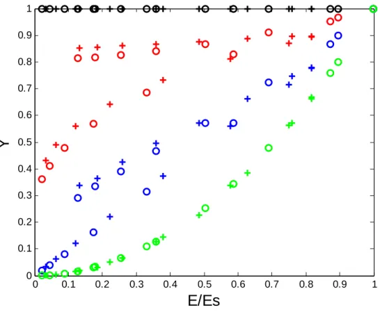
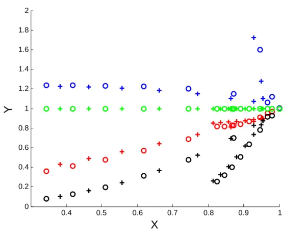
The figure 3 represents Y against the ratio E E/ _S

(

1≤ ≤n 4

)

. The dots for n=1 are trivial (M₁n/M_n =1). One may observe that:

- The curves for spheroids and cylinders are very close

- The curve for n=4 is monotonous. It is a consequence of the Cauchy’s formula that can be expressed for any convex body: Y =

(

E E/ _S

)

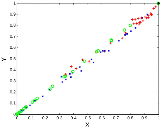
2.

- The curves for n=2 and n=3 present two branches, one for elongated spheroids or cylinders and one for flat spheroids or cylinders. As a consequence, E E may not be the only variable / S

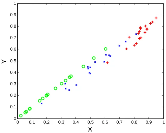
determining Y. The behaviour of extreme cases (very thin disc and very long needle) suggests that the relevant variable could be X =

(

E E/ _S

) (

α C C/ _S

)

β. The figure 4 represents Y versus this new variable X. The standard deviation σ (i.e. the root mean square relative deviation) calculated from the data corresponding to the N=32 spheroids and cylinders, is defined as

(

) (

)

(

)

2 1, 1 i/ S i/ S / i / i N E E α C C β Y N

σ

= =

∑

− (14)

The (

α

,

β

) values, corresponding to the smallest

σ

, are gathered in the table 2; they depend on the moment order n:

(

α β

,

) (

=

α β

n, n

)

. However, the peculiarity of the CLD function for the highest values of chord length in the case of very elongated cylinders leads to a small deviation from Cauchy formula (Eq.12) caused by a tricky numerical integration. The relative

deviation 2 0 4 12 1 V M S M

π

− remains smaller than 0.03 for the cylinder with h/2R=128. Therefore the

σ

value for n=4 (Table 2) is not equal to 0.

n / (

α,β

)

α

β

σ

1 0 0 0

2 0.30 0.225 0.05

3 1.05 0.525 0.06

4 2 0 0.005

Table 2: exponents (

α,β

) in X =

(

E E/ _S

) (

α C C/ _S

)

β for the nth moments. cylinders and spheroids (analytical CLD).

σ

is the standard deviation (see text).

This leads to the following approximate expression for spheroids and cylinders:

(

1 /

) (

/ 1 /

)

(

/

) (

/

)

n n

n n

n S nS S S

Y = M M M M = E E α C C β (15)

Our results may be compared with the inclusion inequalities of Heinrich [31] in the case of three-dimensional space. He proposed two inclusion expressions ((15) and (17) in [31]) that are conjectures. The difference between the two expressions is located in the lower bound:

(

)

2( )1 / 3 / n 1 n S w E E − ≤ ≤Y (15-Heinrich) (16) and

(

)

2( )1 / 3

₍

_{) (}

2

₎

4 / n / n / n n S n S S w E E − ≤ ≤Y v E E − C C − (17-Heinrich) (17) With

(

)

4 3 n/ 4 n n v = −

π

u (18) ( )

(

)

2( )1 / 3 4 / 3 3 3 4 / n n n n w =

κ

− −

π

− − u (19) And 2 2 2 3 3 2 3 3 n n n n n u

κ

κ

κ κ κ

+

κ

  =     (20) and

(

)

/ 2 / 1 / 2 m m m

κ

=

π

Γ + (21)

In this new formulation, the lower bounds are the same for (15-Heinrich) and (17-Heinrich), whereas the upper bounds are different. Following Heinrich ([31], page 8266), (15-Heinrich) should be used as an optimal upper bound for n=2 and (17-Heinrich) for n=3. This conjecture is well verified for spheroids and cylinders for n=2 (Figure 5a) and n=3 (Figure 5b). In the figures 5a-b, the red dots correspond to the raw values ( E C Y ) for each body. The i, i, i

approximation (Eq.15) corresponds to the bisector in the X-Y graph. The two branches of the lower and upper bounds correspond to prolate and oblate spheroids (long and flat cylinders).

3.3. Behaviour of bodies with any shape

The set of bodies described in section 2 is now considered. Table 1 contains all the raw data concerning these bodies: 10 spheroids and cylinders, 18 facetted bodies. CLD moments are calculated from CLD obtained by MCS. We will separately examine the set of facetted bodies. The figure 6 represents the dimensionless moments Y versus the variable X for this set by

keeping the

(

α β

,

)

parameters values reported in table 2. The standard deviation

σ

is equal to 0.14 (n=2) and 0.167 (n=3). This large deviation does not correspond to a statistical scattering, but to a deterministic shift of the curve. This concerns all the dots in the graph. In order to identify the cause of this discrepancy, the ratio Y/X for all the bodies, including spheroids and cylinders, has been reported in the figure 7a. Y is obtained by MC simulations. We may see the relationship between this ratio and the type of body shape. We suggest that this observation is due to the presence of edges and the vertices in the facetted bodies and we retain as relevant additional parameter the number of vertices Nc. It must be kept in mind that

the vertices do not contribute to W2. Figure 7b represents Y/X versus

1 c

N− . It can be seen that

Y/X is roughly a decreasing function of 1 c

N− . Moreover, the results for the 3rd order moment are close to the ones for the 2nd order moment. So, a corrected expression 15 is considered:

(

1 /

) (

/ 1 /

)

( )(

/

) (

/

)

n n

n n

n S nS c S S

Y = M M M M = f N E E α C C β (22)

The function f has to fulfil the following requirements:

- The Cauchy formula are respected: f N

( )

c =1 for n=1 and n=4

- f N

( )

_c =1 for bodies without corner (spheroids and cylinders) ; these bodies will be considered as polyhedra with an infinite number of vertices

-

(

α β

_n, _n

)

are the same for any convex body. We choose the following expression for f:

n / (

α,β

)

α

β

σ

(18) Facetted bodies deviation from Eq. 15

σ

(18) Facetted bodies deviation from Eqs 22-23

σ

All (28) bodies deviation from Eqs 22-23 1 0 0 0 0 0 2 0.30 0.225 0.14 0.043 0.043 3 1.05 0.525 0.167 0.064 0.06 4 2 0 0.013 0.013 0.013

Table 3: exponents (

α,β

) in X =

(

E E/ _S

) (

α C C/ _S

)

β for the nth moments. bodies from Table 1 (CLD from MCS). Standard deviation

σ

related to different models (Eq.15 and Eqs.22-23).

The present results have been compared with the inclusion inequalities of Heinrich in figures 8a (n=2) and 8b (n=3). The red dots correspond to the raw values (E C Y ) for each body. _i, _i, _i

Our results are yet consistent with the findings of Heinrich.

4. Conclusion

We have shown that the CLD moments are related to the Minkowski functionals by means of an empirical expression. However, if this approximation works reasonably well for rounded bodies, it is less applicable to polytopes. A better approximation must consider an additional parameter as the vertex number of the body. As a consequence, we propose a simple empirical expression relating Mn to n, S, V, W2, Nc that represents MCS data with an accuracy of 5%.

CLD is a non monotone function; it can have discontinuities. So, it is not so surprising that the Minkowski functional set is not sufficient to represent the CLD moments. As it is, we

have no explanation about the form of the empirical expression and the values of the fitting parameters (

α β

_n, _n,A) as well. This is a challenging task to give answers to these questions. At this stage the empirical expression can be only used to evaluate the second and third order CLD moments of convex bodies for practical applications.

Acknowledgments: The authors would like to thank the professor Debayle for his valuable

References

[1] A.M. Kellerer, Chord Length Distributions and related quantities for spheroids, Radiation Research, 98(1984)425-437

[2] W. Gille, Particle and Particle systems characterization: Small-Angle Scattering (SAS) Applications, CRC Press, 2013.

[3] S. Jacquier & F. Gruy, Application of scattering theories to the characterization of precipitation processes, Light Scattering Reviews 5, pp37-78, 2010, Ed. A. Kokhanovsky, Springer

[4] V.K. Ohanyan and N.G. Aharonyan Tomography of bounded convex domains, International Journal of Mathematical Science Education 2(2009)1-12

[5] U. Bäsel, Random chords and point distances in regular polygons, Acta Math. Univ. Comenianae 83(2014)1-18

[6] W. Gille, The small-angle scattering correlation function of the hemisphere, Computational Materials Science, 15(1999)449-454

[7] W. Gille, Chord length distributions of infinitely long geometric figures, Powder Technology 123(2002)292-298

[8] W. Gille, Chord length distribution density of a triangular rod, Computational Materials Science 22(2001)151-154

[9] R. Garcia-Pelayo, Distribution of distance in the spheroid, J. of Physics A: Mathematical and General, 38(2005)3475-3482

[10] H.S. Sukiasian Three-dimensional Pleijel identity and its application, Izvestiya Natsionalnoi Akademii Nauk Armenii Matematika 38(2003)53-69

[11] S. Ciccariello, The chord-length probability density of the regular octahedron, J. Appl. Cryst. 47(2014)1216-1227

[12] R. Kirste and G. Porod, Röntgenkleinwinkelstreuung an Kolloiden Systemen. Asymptotisches Verhalten der Streukurven, Kolloid Zeitschrift & Zeitschrift für Polymere 184(1962)1-7

[13] H. Wu and P.W. Schmidt, Intersect distributions and small-angle X-ray scattering theory, J. Appl. Cryst. 4(1971)224-231

[14] H. Wu and P.W. Schmidt, The relation between the particle shape and the outer part of the small-angle X-ray scattering curve, J. Appl. Cryst. 7(1974)131-146

[15] S. Ciccariello, Deviations from the Porod law due to parallel equidistant interfaces, Acta Cryst. A41(1985)560-568

[16] S. Ciccariello and A. Benedetti, Parametrizations of scattering intensities and values of the angularities and of the interphase surfaces for three-component amorphous samples, J. Appl. Cryst. 18(1985)219-229

[17] S. Ciccariello, The leading asymptotic term of the small-angle intensities scattered by some idealized systems, J. Appl. Cryst. 24(1991)509-515

[18] R. Sobry, J. Ledent and F. Fontaine, Application of an extended Porod law to the study of the ionic aggregates in telechelic ionomers, J. Appl. Cryst. 24(1991)516-525

[19] S. Ciccariello, Edge contributions to the Kirste-Porod formula: the truncated circular right cone case, Acta Cryst. A49(1993)398-405

[20] R. Sobry, F. Fontaine and J. Ledent, Extension of Kirste-Porod’s law in the case of angulous interfaces, J. Appl. Cryst. 27(1994)482-491

[23] M. Hyksova, A. Kalousova, I. Saxl, Early history of geometric probability and stereology, Image Anal. Stereol. 31(2012)1-16

[24] L.A. Santalo, Integral geometry and geometric probability, 2004, Cambridge Mathematical Library

[25] H. Hadwiger, Vorlesungen über Inhalt, Oberfläche und Isoperimetrie, Springer, Berlin, 1957.

[26] G.E. Schröder-Turk, W. Mickel, S.C. Kapfer, F.M. Schaller, B. Breidenbach, D. Hug, K. Mecke, Minkowski tensors of anisotropic spatial structure, arXiv:1009.2340v5 [cond-mat-soft] 6 Aug 2013

[27] C.H Arns, M.A. Knackstedt, K.R. Mecke, Characterization of irregular spatial structures by parallel sets and integral geometric measures, Colloids and surfaces A: Physicochem. Eng. Aspects 241(2004)351-372

[28] F. Voss and L. Cruz-Orive, Second moment formulae for geometric sampling with test probes, Statistics 43(2009)329-365

[29] L. Heinrich, On lower bounds of second-order chord power integrals of convex discs, Rendiconti del Circolo Matematico di Palermo Series II, Suppl. 81(2009)213 - 222.

[30] L. Heinrich, Some new results on second-order chord power integrals of convex quadrangles, Rendiconti del Circolo Matematico di Palermo Series II, Suppl. 84(2012)195 - 205.

[31] L. Heinrich, Lower and upper bounds for chord power integrals of ellipsoids, Applied Mathematical Sciences, 8(2014)8257-8269

[32] A. Mazzolo and B. Roesslinger, Monte Carlo simulation of the chord length distribution function across convex bodies, non convex bodies and random media, Monte Carlo Methods and Applications, 10(2004)443-454

[33] E.T. Jaynes, The well posed problem, Papers on Probability, Statistics and Statistical Physics, R.D. Rosencrantz Ed, D. Reidel, Dordrecht (1983)133-148

[34] http://mathworld.wolfram.com/Ellipsoid.html

[35] I. Rivin, Surface area and other measures of ellipsoids, Advances in Applied Mathematics 39(2007)409-427

[36] C. Redenbach, A. Rack, K. Schladitz, O. Wirjadi, M. Godehardt, Beyond imaging: on the quantitative analysis of tomographic volume data, Int. J. Mat. Res. 103(2012)217-227

0 5 10 15 20 25 30 0.997 0.998 0.999 1 1.001 1.002 1.003

body N

M

1

,C

/M

1

,M

C

S

Figure 1: CLD 1st order moment; ratio between Cauchy value and the one coming from Monte Carlo Simulation versus the number N of the body; the numbering corresponds to the raw position in table 1.

0 5 10 15 20 25 30 0.97 0.98 0.99 1 1.01 1.02 1.03

body N

M

4

,C

/M

4

,M

C

S

Figure 2: CLD 4th moment; ratio between Cauchy value and the one coming from Monte Carlo Simulation versus the number N of the body; the numbering corresponds to the raw position in table 1.

0 0.1 0.2 0.3 0.4 0.5 0.6 0.7 0.8 0.9 1 0 0.1 0.2 0.3 0.4 0.5 0.6 0.7 0.8 0.9 1

E/Es

Y

Figure 3: ratio Y =

(

M₁n/M_n

) (

/ M₁n_S/M_nS

)

versus E E ; n is the order of the moment; n=1, / _S 2, 3 or 4. + corresponds to cylinders, o corresponds to spheroids. n=1: black; red: n=2; blue:

0 0.1 0.2 0.3 0.4 0.5 0.6 0.7 0.8 0.9 1 0 0.1 0.2 0.3 0.4 0.5 0.6 0.7 0.8 0.9 1

X

Y

Figure 4: ratio

(

₁n/

) (

/ ₁n /

)

n S nS

Y = M M M M versus X =

(

E E/ _S

) (

α C C/ _S

)

β; n is the order of the moment; n=2,3 or 4; red,+: n=2; blue,x: n=3; green,o: n=4. Cylinders and Spheroids. (

α,β

) from table 2.

0.4 0.5 0.6 0.7 0.8 0.9 1 0 0.2 0.4 0.6 0.8 1 1.2 1.4 1.6 1.8 2

X

Y

Figure 5a: ratio

(

₁n/

) (

/ ₁n /

)

n S nS

Y = M M M M versus X =

(

E E/ _S

) (

α C C/ _S

)

β; n is the order of the moment; n=2. + corresponds to cylinders, o corresponds to spheroids. red: this work; black: lower bound (Heinrich [31], Eq.15-17); blue: upper limit. (Heinrich [31], Eq.17); green: upper limit. (Heinrich [31], Eq.15)

0 0.1 0.2 0.3 0.4 0.5 0.6 0.7 0.8 0.9 1 0 0.1 0.2 0.3 0.4 0.5 0.6 0.7 0.8 0.9 1

X

Y

Figure 5b: ratio

(

₁n/

) (

/ ₁n /

)

n S nS

Y = M M M M versus X =

(

E E/ _S

) (

α C C/ _S

)

β; n is the order of the moment; n=3. + corresponds to cylinders, o corresponds to spheroids. red: this work; black: lower bound (Heinrich [31], Eq.15-17); blue: upper limit. (Heinrich [31], Eq.17); green: upper limit. (Heinrich [31], Eq.15)

0 0.1 0.2 0.3 0.4 0.5 0.6 0.7 0.8 0.9 1 0 0.1 0.2 0.3 0.4 0.5 0.6 0.7 0.8 0.9 1

X

Y

Figure 6: ratio Y =

(

M₁n/M_n

) (

/ M₁n_S /M_nS

)

versus X =

(

E E/ _S

) (

α C C/ _S

)

β; n is the order of the moment; n=2,3 or 4; red,+: n=2; blue,x: n=3; green,o: n=4. Facetted bodies from Table 1.

0 5 10 15 20 25 30 0.65 0.7 0.75 0.8 0.85 0.9 0.95 1 1.05

body N

Y

(M

C

S

)/

X

Figure 7a: Y(MCS)/X versus the number of the body : N=1(sphere); N=2-6(cylinders);

N=7-10(spheroids); N=11-15(parallelepipeds); N=16(octahedron); N=17-19(pyramids); N=20-23(prisms); N=24-28(bipyramids). * black: n=2; + red: n=3.

0 0.05 0.1 0.15 0.2 0.25 0.3 0.35 0.65 0.7 0.75 0.8 0.85 0.9 0.95 1 1.05

1/Nc

Y

(M

C

S

)/

X

Figure 7b: Y(MCS)/X versus the reciprocal of vertex number : * black: n=2; + red: n=3. The

dots for n=3 are shifted to the right for greater clarity. The second column, shifted to the right for greater clarity, corresponds to cylinders.

0.65 0.7 0.75 0.8 0.85 0.9 0.95 1 0 0.5 1 1.5 2 2.5 3

Figure 8a: ratio

(

₁n/

) (

/ ₁n /

)

n S nS

Y = M M M M versus X =

(

E E/ _S

) (

α C C/ _S

)

β; n is the order of the moment; n=2. bodies from table 1. red: this work; black: lower bound (Heinrich [31], Eq.15-17); blue: upper limit. (Heinrich [31], Eq.17); green: upper limit. (Heinrich [31], Eq.15)

0.1 0.2 0.3 0.4 0.5 0.6 0.7 0.8 0.9 0 0.1 0.2 0.3 0.4 0.5 0.6 0.7 0.8 0.9 1

X

Y

Figure 8b: ratio

(

₁n/

) (

/ ₁n /

)

n S nS

Y = M M M M versusX =

(

E E/ _S

) (

α C C/ _S

)

β; n is the order of the moment; n=3. Bodies from table 1. red: this work; black: lower bound (Heinrich [31], Eq.15-17); blue: upper limit. (Heinrich [31], Eq.17); green: upper limit. (Heinrich [31], Eq.15)