Titre:
Title
:
A sampling-based exact algorithm for the solution of the minimax
diameter clustering problem
Auteurs:
Authors
: Daniel Aloise et Claudio Contardo
Date: 2018
Type:
Article de revue / Journal articleRéférence:
Citation
:
Aloise, D. & Contardo, C. (2018). A sampling-based exact algorithm for the solution of the minimax diameter clustering problem. Journal of Global Optimization, 71(3), p. 613-630. doi:10.1007/s10898-018-0634-1
Document en libre accès dans PolyPublie
Open Access document in PolyPublie
URL de PolyPublie:
PolyPublie URL: https://publications.polymtl.ca/3251/
Version: Version finale avant publication / Accepted versionRévisé par les pairs / Refereed Conditions d’utilisation:
Terms of Use: Tous droits réservés / All rights reserved
Document publié chez l’éditeur officiel
Document issued by the official publisher
Titre de la revue:
Journal Title: Journal of Global Optimization (vol. 71, no 3)
Maison d’édition:
Publisher: Springer
URL officiel:
Official URL: https://doi.org/10.1007/s10898-018-0634-1
Mention légale:
Legal notice:
This is a post-peer-review, pre -copyedit version of an article published in Journal of Global Optimization. The final authenticated version is available online at:
https://doi.org/10.1007/s10898-018-0634-1
Ce fichier a été téléchargé à partir de PolyPublie, le dépôt institutionnel de Polytechnique Montréal
This file has been downloaded from PolyPublie, the institutional repository of Polytechnique Montréal
(will be inserted by the editor)
A sampling-based exact algorithm for the solution of the
minimax diameter clustering problem
Daniel Aloise · Claudio Contardo
Received:February 20, 2018/ Accepted:
Abstract We consider the problem of clustering a set of points so as to mini-mize the maximum intra-cluster dissimilarity, which is strongly NP-hard. Ex-act algorithms for this problem can handle datasets containing up to a few thousand observations, largely insufficient for the nowadays needs. The most popular heuristic for this problem, the complete-linkage hierarchical algorithm, provides feasible solutions that are usually far from optimal. We introduce a sampling-based exact algorithm aimed at solving large-sized datasets. The algorithm alternates between the solution of an exact procedure on a small sample of points, and a heuristic procedure to prove the optimality of the current solution. Our computational experience shows that our algorithm is capable of solving to optimality problems containing more than 500,000 ob-servations within moderate time limits, this is two orders of magnitude larger than the limits of previous exact methods.
Keywords clustering · diameter · large-scale optimization
1 Introduction
Clustering is one of the most essential tasks in data mining and machine learning (Anderberg 1973; Kaufman and Rousseeuw 1990). It involves the reading and treatment of unlabeled observations so as to identify hidden and non-obvious patterns that could otherwise not be found by simple inspection
D. Aloise
D´epartement de g´enie informatique et g´enie logiciel ´
Ecole Polytechnique de Montr´eal, QC, Canada E-mail: daniel.aloise@gerad.ca
C. Contardo
D´epartement de management et technologie ESG UQ `AM, Montr´eal, QC, Canada E-mail: claudio.contardo@gerad.ca
of the data. It is often used at the first stages of mining procedures with the objective of labeling the data for further mining using more sophisticated models and algorithms.
In its simplest form, a clustering problem can be formally defined as follows. We are given a positive integer K > 1 representing the number of sought clusters. We are also given a set V of observations, and we denote by P(V ) the set of K-partitions of V , this is partitions composed of exactly K subsets each. Let f : P(V ) −→ R be a real-valued function. The objective is to find a K-partition P∗= {Pi∗}K
i=1 ∈ P(V ) such that P∗∈ arg min{f (P ) : P ∈ P(V )}.
The function f is usually described by means of a symmetric dissimilarity matrix d : V × V −→ R+. The dissimilarity duv of two observations u, v ∈ V
indicates the degree of discrepancy between them. For a partition P = {Pi}Ki=1,
the maximum diameter is defined as Dmax(P ) = max{max{duv: u, v ∈ Pk} :
1 ≤ k ≤ K}. The minimax diameter clustering problem (MMDCP) is the problem of finding a partition P∗∈ arg min{Dmax(P ) : P ∈ P(V )}.
The classic book of Garey and Johnson (1979) refers to the MMDCP as the clustering problem, to prove that the associated decision problem is strongly NP-complete. This highlights the historical importance of the MMDCP which is perhaps the most intuitive among clustering criteria.
Existing exact algorithms for the MMDCP have little practical use as they can only handle problems containing up to a few thousand observations. The state-of-the-art algorithm for this problem based on constraint programming is capable of solving problems containing up to 5,000 observations (Dao et al 2017).
In this article we present an exact method for the MMDCP that typically runs in a time that is comparable to the time needed to compute the associ-ated dissimilarity matrix and that, moreover, consumes only a limited amount of memory resources. The algorithm iterates between the execution of an ex-act clustering routine performed on a sampling of the objects, and that of a heuristic routine used to enlarge that sampling if deemed necessary.
The remainder of this article is organized as follows. In Section 2 we pro-vide a literature review on exact and heuristic algorithms for the MMDCP and related problems, as well as on uses of sampling-based algorithms within exact frameworks. In Section 3 we present our algorithmic framework and provide guarantees on the quality of the solutions obtained by the method. In Section 4 we present in detail the algorithm used in the exact subroutine of the method. In Section 5 we present the heuristic subroutine used to prove the optimality of the current sample, or to enlarge it. In Section 6 we mention some acceler-ation techniques used. In Section 7 we present some computacceler-ational evidence of the usefulness of our method. In Section 8 we briefly discuss the limitations encountered during the testing phase of our method. Section 9 concludes our paper and provides insights on potential avenues for future research.
2 Literature review
The MMDCP is traditionally handled using an agglomerative hierarchical al-gorithm, namely the complete-linkage algorithm. This algorithm begins with every point in V belonging to a single cluster, and then iteratively merges the two nodes u, v of minimum dissimilarity. Each time that a merge occurs, the dissimilarity matrix is updated by removing one column and one row as-sociated with one of the two nodes merged. The remaining row and column corresponds to a merged node z = {u, v}. The dissimilarity between a point w and the merged node z is set to dwz← max{dwu, dwv}. A na¨ıve
implemen-tation of this algorithm runs in O(n3) time and uses O(n2) space (Johnson
1967). A specialized implementation of the algorithm runs in O(n2) time and
uses O(n) space (Sibson 1973; Defays 1977). The complete-linkage algorithm is a heuristic for the MMDCP and seldom finds optimal solutions as reported by Alpert and Kahng (1997); Hansen and Delattre (1978).
The FPF (Furthest Point First ) method introduced in Gonzalez (1985) for the solutions of the MMDCP works with the idea of head objects for each cluster of the partition to which each object is assigned. In the first iteration, an object is chosen at random as the head of the first cluster and all objects assigned to it. In the next iteration, the furthest object from the first head is chosen as the head of the second cluster. Then, any object which is closer to the second head than to the first one is assigned to the second cluster. The algorithm continues for K iterations, choosing the object which is the furthest to its head as the head of the new cluster. The FPF heuristic is guaranteed to find a partition with diameter at most two times larger than the diameter of the optimal partition.
Regarding exact methods for the MMDCP, Hansen and Delattre (1978) explore the relationship between diameter minimization and graph-coloring to devise a branch-and-bound method to solve problems of non-trivial size. Br-usco and Stahl (2006) proposes a backtracking algorithm, denoted Repetitive Branch-and-Bound Algorithm (RBBA), that branches by assigning each ob-ject to one of the possible K clusters. Pruning is performed whenever: (i) the number of unassigned objects is smaller than the number of empty clusters; (ii) the assignment of an object to a particular cluster yields a partition with a diameter larger than the diameter of the best current branch-and-bound so-lution; and (iii) there is an unassigned object that cannot be assigned to any of the clusters of the partial solution. Recently, Dao et al (2017) proposed a constraint programming approach for the MMDCP whose computational per-formance outranked the previous exact approaches found in the literature. In particular, the method obtained the optimal partitions for many benchmark instances, the largest of which with 5,000 objects grouped in three clusters.
Iterative sampling is a method that ignores parts of the problem and solves a restricted master problem (RMP) of usually much smaller size. It then ex-ecutes a subproblem (SP) that either proves the optimality of the solution associated with the RMP, or enlarges it by adding the parts that were wrongly ignored. Lozano and Smith (2017) used this idea to solve a shortest path
inter-diction problem. The algorithm samples paths that are likely to be attacked by an attacker. The paths that are not identified as such are ignored and thus the associated restricted problem (a MIP) contains much fewer binary vari-ables than the original problem. The optimality of the solution is validated by solving a shortest path problem. The algorithm showed very good results as it was capable to scale and solve problems several orders of magnitude larger than earlier methods.
Our algorithm is inspired form the need of handling large datasets. We are not the first to elaborate upon the need of developing a scalable algorithm able to handle large datasets while avoiding as much as possible the scanning of the whole data. Zhang et al (1997) use a tree structure to estimate and store the distribution of the dissimilarities. Their algorithm then relies on this estimator to proceed to cluster the data. In Bradley et al (1998), the authors introduce an algorithm for the k-means clustering problem that uses compression and discarding of data to reduce the number of observations. Fraley et al (2005) introduce a sampling-based algorithm to solve problems containing large amounts of data in a sequential fashion. At every iteration of their algorithm, typically much smaller datasets are considered. Unlike our method, all these algorithms are heuristic in nature.
3 Iterative sampling
The iterative sampling method uses an exact and a heuristic procedure inter-changeably to find a small sample whose optimal solution is that of the original problem, and to build an optimal solution from enlarging that sample. Let us denote by (Q) the problem
ω∗= min{Dmax(P ) : P ∈ P(V )}. (1)
For a given sample U ⊆ V , we let Q(U ) the problem Q restricted to the sample U , ω∗(U ) be its optimal value and P∗(U ) its optimal solution.
For a given initial sample U0(that might be empty, but is indeed initialized
to contain K + 1 nodes as explained in detail in Section 6), we set U ← U0
and t ← 0. At iteration t, one solves problem Q(U ) to optimality. A heuristic procedure iteratively enlarges the partition P∗(U ) and tries to build a feasible solution for problem Q of cost ω∗(U ). If all nodes in V \ U can be inserted into one cluster of P∗(U ) without entailing an increase of the objective, the resulting partition is returned. Otherwise the set U is enlarged, we let t ← t+1 and the same process is applied again on the enlarged sample. The following pseudo-code illustrates the method:
Algorithm 1 Iterative sampling Require: V, K
Ensure: Optimal K-partition P∗= {Pi∗: i = 1 . . . K} of V U ← U0 ω∗(U ), ω∗← ∞ P∗(U ), P∗← ∅ W ← ∅ repeat U ← U ∪ W (ω∗(U ), P∗(U )) ← ExactClustering(U ) (ω∗, P∗, W ) ← HeuristicClustering(P∗(U ), V \ U ) until W = ∅ return P∗
In this algorithm, procedure ExactClustering(U) solves problem Q(U ) to optimality for a given sample U of V . It returns the optimal solution P∗(U ) and its objective value ω∗(U ). The function HeuristicClustering(P∗(U ), V \ U ) completes the solution found by ExactClustering(U) and returns the resulting partition P∗ (not necessarily an optimal one), its value ω∗ and a set W containing the nodes that could not be inserted into P∗(U ) without increasing its maximum diameter (∅ if no such node exists). The next two results support the exactness and finiteness of our approach:
Lemma 1 For any sample U ⊆ V , ω∗(U ) ≤ ω∗.
Proof Let P∗ = (Pi∗)Ki=1 be an optimal clustering of V . Then the clustering R = (U ∩Pi∗)Ki=1is a clustering of U of smaller diameter or equivalent diameter
ω∗. It follows that ω∗(U ) ≤ ω∗. ut
Proposition 1 The iterative sampling method ends in a finite number of it-erations and returns an optimal clustering of V .
Proof At every iteration, procedure HeuristicClustering(P∗(U ), V \ U ) either proves the optimality of the current subproblem (if it returns W = ∅), or the set U is augmented. In the worst case, U will grow up to become equal to V , in which case procedure ExactClustering(U) is guaranteed to return
an optimal solution of the problem. ut
Remark 1 A simple worst-case time analysis of our method would suggest that it is indeed theoretically slower than solving the complete problem at once. In practice, one would expect the iterative sampling method to exploit the high degeneracy of the MMDCP to prove optimality after a few iterations. In this case, procedure ExactClustering(U) solves problems several orders of magnitude smaller than the original one.
4 Sub-routine ExactClustering(U): Branch-and-price
In this section we describe an exact algorithm for the MMDCP used as the exact subroutine within the iterative sampling framework. The algorithm is based on the solution of a set-covering formulation of the MMDCP by branch-and-price. We first include a high-level description of our branch-and-price algorithm. Second, we introduce the set-covering formulation of the problem. In the following subsections we describe the different parts of the method, namely the pricing and branching schemes.
4.1 High-level description of column generation
A branch-and-price algorithm is a LP-based branch-and-bound algorithm in which lower bounds are computed by solving a LP by column generation (CG). In CG, one solves iteratively a restricted master problem (RMP) and a pricing subproblem (PS). Usually, the RMP is associated to an integer-linear program (ILP) for which the integrality constraints are relaxed, and for which only a subset of variables is considered. In our case, the ILP corresponds to a set-covering problem SC(U, K) which, if solved explicitly for the whole set of variables, would return an optimal K-clustering of the nodes in U . Let C denote the set all possible covers of U , and let C0⊆ C denote a subset of those covers. Let RM P (U, K, C0) denote the RMP associated to the covers defined in C0. Let (x, µ) denote the fractional primal and dual solutions associated with RM P (U, K, C0). Let P S(µ) denote the pricing subproblem constructed
from using the dual variables µ to build covers of negative reduced cost. Let X denote the set of columns of negative reduced cost as found by P S(µ). The following pseudo-code is a high-level description of a column generation algorithm:
Algorithm 2 Column generation Require: U, K
Ensure: Optimal solution x of RM P (U, K, C) C0←− C 0 X ←− ∅ repeat C0← C0∪ X (x, µ) ←− RM P (U, C0) X ←− P S(µ) until X = ∅ (x, µ) ←− RM P (U, C0) return x
This CG is then embedded into a branch-and-bound algorithm, for which is necessary to define proper branching rules. In our case, this part is explained in detail in Section 4.5.
4.2 Set-covering formulation of the MMDCP
We are given a sample U of V . We denote by E the set of undirected edges linking any two nodes in U . A cluster can either be equal to a singleton {u} or to a pair (S, e) ∈ P(U ) × E, where e represents one possible edge of maximum diameter within the nodes in S. The set of all feasible clusters containing two or more nodes is denoted by C. For a cluster t = (S, e) ∈ C we denote St= S, et= e.
For every u ∈ U , we let su be a binary variable equal to 1 iff node u is
clustered alone, and we let dube its diameter (as we will explain in Section 4.5,
a node can have a strictly positive diameter following a branching decision). For a given edge e = {u, v} ∈ E, dedenotes the dissimilarity between nodes u
and v. For every t ∈ C we consider a binary variable ztthat will take the value
1 iff the cluster t is retained. For every node u ∈ U we let aut be a binary
constant that takes the value 1 iff u ∈ St. Also, for every edge e ∈ E we let
bet be a binary constant that takes the value 1 iff e = et. We finally define
a continuous variable ω equal to the maximum diameter among the chosen clusters. The MMDCP restricted to the sample U (or equivalently problem Q(U ), as defined in Section 3) can thus be formulated as follows:
min s,ω,z ω (2) subject to ω −X t∈C betdezt≥ 0 e ∈ E (3) ω − dusu≥ 0 u ∈ U (4) X t∈C autzt+ su= 1 u ∈ U (5) X t∈C zt+ X u∈U su= K (6) zt≥ 0 t ∈ C (7) zt is integer t ∈ C (8)
Constraints 3 state that the maximum diameter is greater or equal to the edge of maximum diameter in cluster t. Constraints 4 ensure that the maximum diameter is also larger than the diameter of node u if it is clustered alone. The set of constraints 5 state that each node belongs to one cluster, and the constraints 6 express that the optimal partition contains exactly K clusters. Without loss of generality, they can be replaced by
X t∈C autzt+ su≥ 1 u ∈ U, and X t∈C zt+ X u∈U su≤ K,
since a covering of the nodes which is not a partition cannot be optimal, and any partition with less than K clusters has objective value greater or equal to the optimal partition with K clusters. By replacing the equality constraint by inequalities, the dual variables associated do never change sign, which results on more stable optimization algorithms.
We solve this problem by means of branch-and-price. The linear relaxation of problem (2)-(8) is solved by column generation, whereas the integrality constraints are imposed through branching.
4.3 Pricing subproblem
Let us assume that the linear relaxation of problem (2)-(8) has been solved restricted to a subset C0 ⊂ C of feasible clusters. We can extract dual variables (σe)e∈E, (αu)u∈U, (λu)u∈U and γ for constraints (3), (4), (5) and (6),
respec-tively. The reduced cost of variables su, zt are denoted as cu, ct, respectively,
and are equal to
cu= duαu− λu− γ (9)
ct= detσet− X
u∈U
autλu− γ (10)
The pricing subproblem is performed in two steps. In the first step, we search for single-node clusters of negative reduced cost. This can be done by simple inspection by evaluating expression (9) for every possible u ∈ U .
If no such cluster exists, the second step of the pricing subproblem searches for a feasible cluster t of minimum reduced cost, this is such that expression (10) is minimized. We formulate this problem as an integer program, as follows. For every u ∈ U , we let xube a binary variable equal to 1 iff u ∈ St. For every
edge e ∈ E we let ye be a binary variable equal to 1 iff e = et. We consider
the following integer program:
min x,y φ = X e∈E σedeye− X u∈U λuxu (11)
subject to X f ∈E dfyf− de(xu+ xv− 1) ≥ 0 e = {u, v} ∈ E (12) 2ye− xu− xv≤ 0 e = {u, v} ∈ E (13) X e∈E ye= 1 (14) xu∈ {0, 1} u ∈ U (15) ye∈ {0, 1} e ∈ E (16)
Now, this pricing subproblem will select one edge e ∈ E (associated to a variable ye= 1) and construct a node subset accordingly (associated to the set
{u ∈ U : xu = 1}). We would like to highlight that, if the edge et = {ut, vt}
is chosen in advance (meaning that yet = 1), one can a priori fix to zero all variables xusuch that max{duut, duvt} > det and to one variables xut, xvt. Let us denote then Ut= {u ∈ U \ {u
t, vt} : max{duut, duvt} ≤ det}. The optimal set of nodes for a fixed etcan be found by solving the following integer program:
max x φ 0(e t) = X u∈Ut λuxu (17) subject to xu+ xv ≤ 1 u, v ∈ Ut, u < v, duv> det (18) xu∈ {0, 1} u ∈ Ut (19)
The relationship between φ and φ0(u
t, vt) is as follows:
φ = min{σede− (φ0(e) + λu+ λv) : e = {u, v} ∈ E} (20)
4.4 Solution of the pricing subproblem
The solution of the pricing subproblem exploits the aforementioned property to derive an efficient heuristic and exact method. It relies on the sorting of the edges in E in increasing order with respect to the quantity σede−λu−λv, with
e = {u, v} ∈ E. The greedy heuristic is several orders of magnitude faster than the exact procedure and is always executed first. The exact princing method is thus only executed when the heuristic fails at finding columns of negative reduced cost.
4.4.1 Greedy heuristic
Our greedy heuristic starts, for every edge e = {u, v} ∈ E, with a cluster containing the nodes u and v, and expanding it while possible.
Set k ← 1, and let ek = {uk, vk} be the k-th element of E. We let C =
current cluster and S the set of nodes that can be inserted into C without exceeding the diameter given by dek. At iteration j + 1, we will set v
∗ ←
arg max{λv : v ∈ S}. We then update C and S as follows: the new cluster
becomes C ← C ∪ {v∗}; the new set S becomes S ← S \ {v ∈ S : dvv∗ > de k}. If S is empty, we check if the reduced cost associated to cluster (C, ek) is
negative. If so, stop and return (C, ek). Otherwise, set k ← k + 1 and restart
unless k > |E|, in which case the algorithm is stopped and no column is returned.
4.4.2 Exact algorithm
Let ω be the linear relaxation value associated with the current set of columns. Let ω∗ be the current upper bound of the problem. We define the absolute gap as the difference ω∗− ω and denote it by gap.
Let k ← 1 and let ek = {uk, vk} be the next edge to inspect. Our exact
algorithm computes a maximum weighted clique on the graph Gk= (Uk, Ek),
with Ek = {e = {u, v} : e ∈ E, u, v ∈ Uk, d
e ≤ dek}. Each node u ∈ U has a weight equal to λu. We compute φ0(ek) using CLIQUER ( ¨Osterg˚ard 2002).
Let us denote ck← σekdek− (φ
0(e
k) + λuk+ λvk) − γ. Depending in the value of ck, three possible cases arise:
1. If ck < 0, then a column (a feasible cluster) of negative reduced cost has
been detected. Stop and return the associated cluster. 2. Else if 0 ≤ ck< gap, then do nothing.
3. Else (i.e. if ck≥ gap), then no column t ∈ C such that et= ek can be part
of an optimal solution improving upon the incumbent. Therefore, edge ek
can be removed from the computation of φ in (20) without compromising the exactness of the algorithm.
In cases 2 and 3, we set k ← k + 1 and restart the procedure with the next available edge. If none, we abort the algorithm and return nil.
4.5 Branch-and-bound
Let ((su)u∈U, (zt)t∈C) be the optimal solution at the end of the column
gener-ation process. Let us define, for every e ∈ E, ye=Pt∈Cbetzt. We also define,
for every edge e = {u, v} ∈ E, xe=Pt∈Cautabtzt. In addition, we define, for
every node u ∈ U , ru=Pe={u,v}|v∈U \{u}ye. The solution might be declared
unfeasible if su, ye, xeor ru are fractional for some edge e or node u.
Depend-ing on the branchDepend-ing decision chosen, the two children problems are built as follows:
1. If su ∈]0, 1[ is the chosen branch: We create two children nodes, namely
su = 0 and su ≥ 1. For su = 0 we remove the variable su from the child
master and from the computation of the reduced costs. For the branch su ≥ 1, we simply add the inequality to the child node. As the variable
therefore no need to consider its dual in the computation of the reduced costs when using expression (9).
2. If ye ∈]0, 1[ is the chosen branch: We create two children nodes, namely
ye= 0 and ye≥ 1. For ye= 0 we remove the edge e from the computation
of φ in (20) and also remove all clusters {(S, e) ∈ C0} from the master
problem. For the branch ye≥ 1, we simply add the following inequality to
the child node:P
t∈Cbetzt≥ 1. Its dual must be taken into account for the
computation of the reduced costs.
3. If xe∈]0, 1[ is the chosen branch, with e = {u, v}: We create two children
nodes, namely xe = 0 and xe = 1. For xe = 0, we need to assure that
u and v will never be on the same cluster. Thus, we remove from the master problem all clusters containing both nodes. In addition, we modify their dissimilarity to be duv ← +∞. For the branch xe = 1, we need to
assure that every cluster containing u will also contain v. We proceed to shrink these two nodes into a single node {uv}, and update its diameter to d{uv} ← du + dv. Also, for every w ∈ V \ {u, v}, we let d{u,v}w ←
max{duw, dvw, d{uv}}. We also remove from the master problem all clusters
containing one of the nodes but not both.
4. If ru ∈]0, 1[ is the chosen branch: We create two children nodes, namely
ru = 0 and ru ≥ 1. For ru = 0, we remove from the master all clusters
(S, e) ∈ C0 such that one of the endpoints of e is equal to u. All edges
{e = {v, w} ∈ E : v = u or w = u} are removed from the computation of φ in (20). For the branch ru ≥ 1, we simply add the following inequality
to the child node: P
t∈C
P
{e={u,v}∈E:v∈S}betzt≥ 1.
We have implemented a hybrid branching strategy that performs strong branching for the first 1000 node separations, and pseudo-cost branching af-terwards.
5 Sub-routine HeuristicClustering(P∗(U ), V \ U ): Completion heuristic
To prove the optimality of the solution associated to the current set U or that another iteration of the algorithm is necessary, we have implemented the following completion heuristic. For every subset S ⊆ V , we let diam(S) = max{duv : u, v ∈ S} be the diameter of set S. We also let P∗(U ) = {Pi∗(U ) :
i = 1 . . . K}, ω∗(U ) be the associated optimal clustering of those nodes and the optimal solution value, respectively. For every node u ∈ V \ U and for every cluster Pi∗(U ) ∈ P∗(U ), we let ν(u, i) = max{duv : v ∈ Pi∗(U )}. For each
u ∈ V \ U , the clusters are sorted in non-decreasing order of ν(u, i), this is ν(u, i1) ≤ ν(u, i2) ≤ · · · ≤ ν(u, iK). In case of a tie among two or more clusters,
we proceed to sort them in non-decreasing order of diameter. Following ties are broken arbitrarily. For every 1 ≤ i ≤ K, we denote by Pi∗(U, u) the i-th cluster according to this ordering. Note that this means that for two different observations u and v, Pi∗(U, u) may represent a different cluster than Pi∗(U, v) (as the clusters are sorted, for each node in V \ U , differently).
The next problem is to define an ordering of the nodes in V \ U . The intuition behind our approach is to sort the nodes so as to favor the detection of insertions that would necessarily entail an increase of the maximum diameter in the early stages of the completion process. For every u ∈ V \ U , we consider the following quantities:
l1(u) = max{0, diam(P1∗(U, u) ∪ {u}) − ω
∗(U )} (21)
l2(u) = diam(P1∗(U, u) ∪ {u}) − diam(P1∗(U, u)) (22)
l3(u) = diam(P1∗(U, u) ∪ {u}) (23)
l4(u) = diam(P1∗(U, u)) (24)
The nodes are sorted in non-increasing order of l1. Ties are broken by
considering l2, l3and l4, in that order. Following ties are broken by considering
the same reasoning with P2∗(U, ·), P3∗(U, ·), and so on.
Let us denote V \ U ← {u1, . . . , us} the nodes in V \ U sorted according
to the aforementioned ordering of nodes. Let j ← 1. Each cluster is inspected according to the ordering defined by the quantities ν(uj, ·). Node uj is thus
inserted in the first cluster where it fits if its addition does not entail an increase in the maximum diameter given by ω∗(U ). If no such cluster exists, the algorithm stops. We check whether the insertion of node uj was not possible
because of another previously inserted node ul, l < j. If no such ul exists,
we return W = {uj}, otherwise we return W = {ul, uj}. If the insertion is,
however, possible, we update the diameter of the cluster involved, let j ← j +1 and restart, unless j reaches s + 1 in which case the algorithm stops and the global optimal clustering is returned.
6 Acceleration techniques
To accelerate the whole procedure, some remarks are in order.
First, a preprocessing of the nodes allows a reduction in the number of items. Indeed, it is possible to discard duplicates (an item is said to be a du-plicate of another if they share the exact same attributes). While for some problems this procedure did not help to reduce the number of points, for oth-ers the reduction reached a 70% of the nodes (KDD cup 10%, from 494,020 to only 145,583 nodes). In addition, we perform dimension reduction by re-moving dimensions whose standard deviations are equal to 0. This happens for a particular dimension only when the same value is given for all items in the dataset. Therefore, removing that dimension does not change the optimal solution value.
Second, the set U may be initialized to contain zero or more nodes from the set V . Indeed, for the MMDCP, it is always preferable to begin with a set U containing at least K + 1 nodes. Any set smaller than that will always have cost 0 (it suffices to cluster all nodes apart). In our implementation we have performed the following procedure to initialize the set U .
1. Compute the centroid u of the points in V . If the i-th dimension of the problem is a numerical variable, we let uibe |V |1 Pu∈V ui. On the contrary,
if it is a categorical variable, we let uito be the mode of the values (ui)u∈V.
2. Let then T be the set containing the ρ = min{5000, |V |} farthest points in V from u. For each p ∈ T , we let Tp be built iteratively as follows: in step
1, Tp= {p}. From step 2 to K + 1, we insert into Tp the node v ∈ V \ Tp
whose closest distance to a node in Tp is maximum.
3. The best possible K-clustering for Tp can be obtained by clustering
to-gether the two nodes u, v ∈ Tp whose dissimilarity is the smallest, and
then all the other K − 1 nodes apart. The dissimilarity duv is then the
value of the optimal clustering for Tp.
This algorithm if executed ρ times would turn to be excessively time con-suming, even for a small number of clusters. Indeed, after each execution of the heuristic, we retain the value ν of the largest clustering diameter found so far. We abort the execution of this algorithm as soon as the constructive heuristic has been executed 100 times without generating a solution of value larger than ν.
Third, we always warm-start the branch-and-price procedure by comput-ing lower and upper bounds for the problem, as follows: An upper bound can be obtained by executing the constructive heuristic introduced in Section 5. Moreover, we have implemented an iterated local search method to improve this solution that uses the LS presented in Fioruci et al (2012), with a per-turbation based on the random selection of diameter nodes (two nodes that have maximum intra-cluster distance) and the reassignment of those nodes to randomly selected clusters. The value achieved by the ILS is then used as a cut-off value for the branch-and-price algorithm. Also, the optimal solution from the previous iteration of the branch-and-price provides a lower bound on the value of the optimal solution at the current iteration (thanks to the monotonicity of the MMDCP). Let ω0 be that lower bound. We enforce it by adding to the master problem the inequality
X
t∈C
X
e∈E0
betzt≥ 1, (25)
where E0 = {e ∈ E : de ≥ ω0}. Certainly, one needs to consider its dual
variable in the computation of the reduced costs for the column generation process.
7 Computational results
The proposed algorithm was programmed in C++ using the GNU g++ com-piler v5.2. The general purpose linear programming solver used by CG was CPLEX 12.6. Maximum weighted cliques necessary to the exact solution of the auxiliary problem are computed using CLIQUER ( ¨Osterg˚ard 2002). The algorithm was compiled and executed in a single core on a machine powered
by an Intel Xeon E5-2637 CPU 3.5 GHz x 16 with 128GB of RAM, running the Oracle Linux OS.
In our experimental analysis, we consider some classical problems from clustering, classification and regression tasks. The summary information of these problems is reported in Table 1. In this table we report the name of the problem (under column labeled P roblem), the number of objects to be clustered (under column labeled n), the number of sought clusters (under column labeled K), the number of dimensions (under column labeled s), and the reference (under column labeled Ref.). The only problems for which a dimensionality reduction could be applied (as explained in Section 6) are: Census (from 41 to 39), Image segm (from 19 to 18), Ionosphere (from 34 to 33), KDD cup 10% (from 41 to 39), and Segmentation (from 19 to 18).
It is important to compare clustering algorithms using classical or well documented benchmark datasets since the hardness of a clustering problem depends not only on the number of objects (n), but also on the number of sought clusters (K) and on how the objects are spread in the space. For ex-ample, if objects are embedded in an Euclidean space and located in very separated clusters, any reasonable exact method should find the optimal so-lution regardless of the number of objects, which would bias any conclusions regarding the performance of the algorithm.
The selected problems contain mixed numerical and categorical data. The dissimilarity between two objects u = (ui)si=1, v = (vi)si=1 is computed as:
duv= v u u t s X i=1 g(ui, vi), (26)
where g(x, y) is equal to (x − y)2if x and y are two numerical values, equal to 1 if x and y are two categorical values whose string representations differ, and equal to 0 if x and y are two categorical values whose string representations are the same. The number of categorical dimensions are reported in parenthesis (whenever > 0) under column s of Table 1.
Remark that storing the whole dissimilarity matrix for dataset Cover type would require approximately 10 TB of memory. Our method does not require such large amount of resources.
To assess the efficiency of our method, thereafter labeled IS, we have de-signed three experiments. In the first experiment, summarized in Table 2, we consider a sequential implementation of our algorithm and compare it against the results of three algorithms: the CP algorithm of Dao et al (2017), the RBBA of Brusco and Stahl (2006) and the BB of Delattre and Hansen (1980) We restrict our analysis to the problems used in the experimental analysis of Dao et al (2017) with no dimensionality reduction. The algorithms were executed on a 3.4 GHz Intel Core i5 processor with 8G Ram running Ubuntu. As one can see from this table, our algorithm takes less than two seconds to solve all the problems, including problem Waveform (v2) that passed from being solved in almost a minute, to only 1.9 seconds.
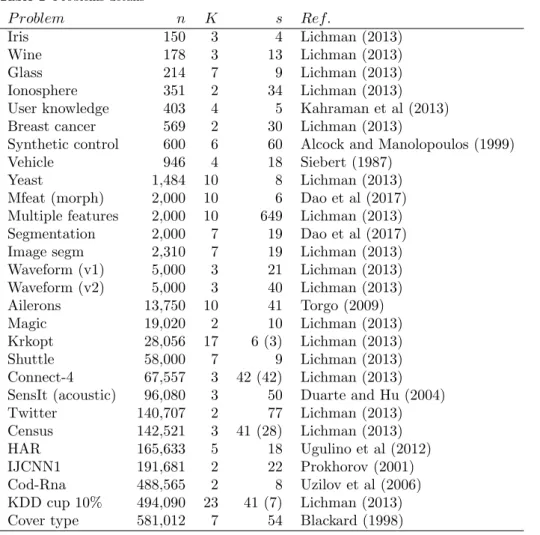
Table 1 Problems details P roblem n K s Ref. Iris 150 3 4 Lichman (2013) Wine 178 3 13 Lichman (2013) Glass 214 7 9 Lichman (2013) Ionosphere 351 2 34 Lichman (2013)
User knowledge 403 4 5 Kahraman et al (2013)
Breast cancer 569 2 30 Lichman (2013)
Synthetic control 600 6 60 Alcock and Manolopoulos (1999)
Vehicle 946 4 18 Siebert (1987)
Yeast 1,484 10 8 Lichman (2013)
Mfeat (morph) 2,000 10 6 Dao et al (2017)
Multiple features 2,000 10 649 Lichman (2013)
Segmentation 2,000 7 19 Dao et al (2017)
Image segm 2,310 7 19 Lichman (2013)
Waveform (v1) 5,000 3 21 Lichman (2013) Waveform (v2) 5,000 3 40 Lichman (2013) Ailerons 13,750 10 41 Torgo (2009) Magic 19,020 2 10 Lichman (2013) Krkopt 28,056 17 6 (3) Lichman (2013) Shuttle 58,000 7 9 Lichman (2013) Connect-4 67,557 3 42 (42) Lichman (2013)
SensIt (acoustic) 96,080 3 50 Duarte and Hu (2004)
Twitter 140,707 2 77 Lichman (2013) Census 142,521 3 41 (28) Lichman (2013) HAR 165,633 5 18 Ugulino et al (2012) IJCNN1 191,681 2 22 Prokhorov (2001) Cod-Rna 488,565 2 8 Uzilov et al (2006) KDD cup 10% 494,090 23 41 (7) Lichman (2013)
Cover type 581,012 7 54 Blackard (1998)
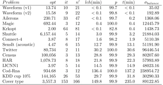
Our second experiment, summarized in Table 3, aims at analyzing the scal-ability of our algorithm for large datasets. We restrict our analysis to problems containing 5,000 objects or more. In this table, label it represents the num-ber of main iterations of our algorithm, this is the numnum-ber of times that the completion heuristic needs to be executed. Label n0 represents the number of objects in the last iteration of the algorithm right before the final comple-tion heuristic takes place. The time (in minutes) spent in the last complecomple-tion heuristic execution is reported under column labeled lch(min). Under column labeled p we report the percentage of objects that are successfully inserted in their closest cluster according to the ordering described in Section 5. This provides a measure of the efficiency of that ordering in the case that the last completion heuristic were aborted prematurely in a heuristic setting. The to-tal running time spent by our algorithm (in minutes) is shown under column
Table 2 Running times (in seconds) on small datasets
P roblem Opt RBBA BB CP IS
Iris 2.6 1.4 1.8 < 0.1 < 0.1 Wine 458.1 2.0 2.3 < 0.1 < 0.1 Glass 5.0 8.1 42.0 0.2 0.2 Ionosphere 8.6 0.6 0.3 0.2 User knowledge 1.2 3.7 0.2 1.1 Breast cancer 2,378.0 1.8 0.5 0.2 Synthetic control 109.4 1.6 0.4 Vehicle 264.8 0.9 0.2 Yeast 0.7 5.2 1.6 Mfeat (morph) 1,595.0 8.59 0.6 Segmentation 436.4 5.7 0.6 Waveform (v2) 15.6 50.1 1.9
Table 3 Detailed results of the iterative sampling method for the MMDCP
P roblem opt it n0 lch(min) p t(min) σbalance
Waveform (v1) 13.74 10 21 < 0.1 99.7 < 0.1 35.02 Waveform (v2) 15.58 9 22 < 0.1 99.8 < 0.1 192.89 Ailerons 230.71 33 47 < 0.1 99.7 0.2 1368.06 Magic 692.44 3 12 0.4 100.0 0.4 12445.79 Krkopt 2.00 64 81 < 0.1 82.8 0.4 1438.73 Shuttle 6,157.44 5 14 3.0 99.9 3.2 21884.03 Connect-4 3.87 8 17 1.6 98.2 1.9 5110.38 SensIt (acoustic) 4.47 6 15 12.7 99.9 13.1 51191.90 Twitter 80,734 2 11 30.2 100.0 30.6 96446.54 Census 100,056 3 13 28.8 99.9 29.3 80207.60 HAR 1,078.73 8 18 21.8 99.9 22.3 57993.89 IJCNN1 3.97 5 14 14.5 99.9 14.9 48023.16 Cod-Rna 934.68 3 12 136.4 100.0 137.2 238954.72 KDD cup 10% 144,165 26 53 29.7 99.9 31.8 30290.33 Cover type 3,557.3 153 166 149.8 99.9 235.0 89122.85
labeled t (min). Finally, column σbalancereports the standard deviation on the
cardinality of the optimal clusters.
As shown in this table, our method is capable of solving all these problems within reasonable time limits. Typically, only very small subsets of V need to be handled by the ExactClustering(U) subroutine at every iteration of the algorithm. In addition, if the last completion heuristic were aborted prema-turely and the remaining objects added into their closest cluster —according to the ordering defined in Section 5—, the resulting heuristic would effectively find the right clustering for a 98.6% of the objects on average.
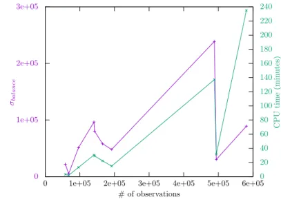
Yet, Figure 1 illustrates the correlation between the time spent by our method and the balance among the different clusters in the optimal solutions.
Fig. 1 Computimes times and balance deviations for different problems
0 1e+05 2e+05 3e+05
0 1e+05 2e+05 3e+05 4e+05 5e+05 6e+050
20 40 60 80 100 120 140 160 180 200 220 240 σbal ance CPU time (min utes) # of observations
We restricted our analysis to problems solved by our method in more than one minute. Indeed, the time spent by the completion heuristic is quadratic on the size of the largest cluster, and consequently, balanced clusters are the best case for proving optimality.
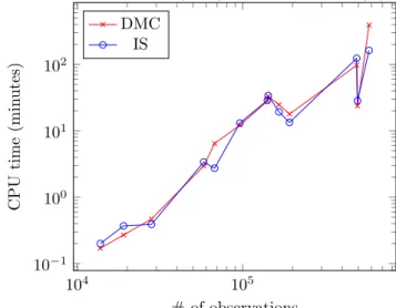
It is important to highlight that our algorithm’s running time for a given dataset is comparable to the time needed to compute its dissimilarity matrix, which is O(n2) time. Moreover, on some very large datasets, it proves even
faster as shown in Figure 2. This demonstrates that it is possible to devise exact methods for the MMDCP that to not need to rely on a pre-computation and storage of the dissimilarity matrix.
Besides establishing new paradigms for the performance of algorithms for the MMDCP, our method also plays an important role on providing bench-mark results for heuristics. In the following experiment, we compare the per-formance of our algorithm against the complete-linkage heuristic (Johnson 1967; Sørensen 1948; Defays 1977). It is well-known that the method seldom finds optimal solutions as reported by Alpert and Kahng (1997); Hansen and Delattre (1978). But how far are its heuristic solutions from optimality? Our third experiment, reported in Table 4, aims at answering this question by con-trasting minimum diameter results obtained by complete-linkage (C-L) and IS on small datasets —those that could be handled by the hclust() routine in R given the available RAM memory. We can notice that minimum diameter partitions provided by the complete-linkage algorithm can be up to ≈ 45% far from optimality, being ≈ 17% worse in average. This is a clear indication of the ineffectiveness of C-L on finding near-optimal solutions for the MMDCP.
Fig. 2 Dissimilarity matrix computation (DMC) vs iterative sampling (IS) 104 105 10−1 100 101 102 # of observations CPU time (min utes) DMC IS
Table 4 C-L and IS on small datasets.
Problem C-L IS rel.dif f.(%) Iris 3.21 2.58 24.42 Wine 665.15 458.13 45.19 Glass 5.69 4.97 14.49 Ionosphere 9.27 8.6 7.79 User knowledge 1.31 1.17 11.97 Breast cancer 2455 2377.96 3.24 Synthetic control 119.82 109.36 9.56 Vehicle 332.28 264.83 25.47 Yeast 0.77 0.67 14.93 Mfeat (morph) 2124.04 1594.96 33.17 Segmentation 442.57 436.4 1.41 Waveform (v1) 15.30 13.74 11.35 Waveform (v2) 17.29 15.58 10.98 Ailerons 295.47 230.71 28.07 Magic 829.69 692.44 19.82 Average 17.46 8 Hard instances
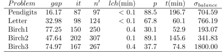
We have encountered difficulties in using our method when trying to solve the MMDCP on problems Pendigits, Letter, Birch1, Birch2 and Birch3 (all of which can be downloaded freely from the UCI benchmark database). Our algorithm stalled after a sufficiently large number of iterations that made the
Table 5 Hard Problems details P roblem n K s Ref. Pendigits 10,992 10 16 Lichman (2013) Letter 20,000 26 16 Lichman (2013) Birch1 100,000 100 2 Zhang et al (1997) Birch2 100,000 100 2 Zhang et al (1997) Birch3 100,000 100 2 Zhang et al (1997)
Table 6 Detailed results of the iterative sampling method for the hard instances
P roblem gap it n0 lch(min) p t(min) σbalance
Pendigits 16.17 87 97 < 0.1 88.5 196.7 704.59
Letter 32.98 98 124 < 0.1 67.8 60.1 766.19
Birch1 77.25 150 250 0.4 30.1 52.9 193.07
Birch2 47.64 202 307 0.1 89.1 145.6 341.83
Birch3 74.97 167 267 0.4 37.7 74.8 1800.00
exact subroutine prohibitively too costly. Table 5 presents the main parameters of these problems.
To be able to execute our algorithm on these datasets and report its re-sults, we performed the following modification to the method (it does not modify in any way the behavior of our algorithm for the already solved in-stances). We added a limit of 1000 nodes in queue in the branching tree of the branch-and-price method. This is not the number of nodes inspected so far, but the number of nodes that remain in queue for separation. When this limit is reachedfor the first time, the completion heuristic is performed fully on the optimal solution obtained for the previous sampling.The optimal solution of ExactClustering(U) on the previous sampling provides a valid lower bound for the problem. The completion heuristic provides an upper bound.
Table 6 reports our results. It contains the same information provided in Table 3, except for column opt which is replaced by column gap referring to the relative difference (in %) between the upper and lower bounds obtained by the algorithm.
All these problems have in common the existence of a large number of alternate solutions for values of the maximum diameter that are close to the optimal value. When this happens, a set W that might induce an increase in the diameter for a given solution might be clustered perfectly fine for some alternate one. In the next iteration, the optimal clustering subroutine will necessarily find an optimal solution of the same value. Moreover, the existence of many such solutions will also harm the resolution process because of the symmetries involved, which is a known weakness of LP-based branch-and-bound methods. We believe that, as a matter of future research, one may implement an alternative algorithm for ExactClustering(U) as, for instance, the CP of Dao et al (2017).
9 Concluding remarks
We have presented an iterative sampling algorithm for the solution of the minimax diameter clustering problem (MMDCP), which is strongly NP-hard. Our implementation of the method outperforms the state-of-the-art algorithm for this problem by solving datasets that are two orders of magnitude larger than those handled by previous schemes. We can identify three potential av-enues for future research: first, to find other uses for the sampling method, either in classification or other areas where set-partitioning problems with high degrees of degeneracy arise frequently; second, in what concerns specif-ically the MMDCP, to work on the robustness of the method to allow the solution of problems with noise; third, to build a heuristic implementation of the method to allow the solution of arbitrarily large datasets, either applied to the MMDCP or to another partitioning problem.
Acknowledgments
This research was financed by the Fonds de recherche du Qu´ebec - Nature et technologies (FRQNT) under grant no 181909 and by the Natural Sciences and Engineering Research Council of Canada (NSERC) under grants 435824-2013 and 2017-05617. These supports are gratefully acknowledged.
References
Alcock R, Manolopoulos Y (1999) Time-series similarity queries employing a feature-based approach. In: 7th Hellenic Conference on Informatics, Ioannina, Greece, pp 27–29 Alpert CJ, Kahng AB (1997) Splitting an ordering into a partition to minimize diameter.
Journal of Classification 14:51–74
Anderberg MR (1973) Cluster analysis for applications / Michael R. Anderberg. Academic Press New York
Blackard JA (1998) Comparison of neural networks and discriminant analysis in predicting forest cover types. PhD thesis, Colorado State University
Bradley PS, Fayyad UM, Reina C (1998) Scaling clustering algorithms to large databases. In: KDD, pp 9–15
Brusco MJ, Stahl S (2006) Branch-and-bound applications in combinatorial data analysis. Springer Science & Business Media
Dao TBH, Duong KC, Vrain C (2017) Constrained clustering by constraint programming. Artificial Intelligence 244:70–94
Defays D (1977) An efficient algorithm for a complete link method. The Computer Journal 20(4):364–366, http://comjnl.oxfordjournals.org/content/20/4/364.full.pdf+html Delattre M, Hansen P (1980) Bicriterion cluster analysis. Pattern Analysis and Machine
Intelligence, IEEE Transactions on 4:277–291
Duarte M, Hu YH (2004) Vehicle classification in distributed sensor networks. Journal of Parallel and Distributed Computing 64:826–838
Fioruci JAA, Toledo FM, Nascimento MACV (2012) Heuristics for minimizing the maximum within-clusters distance. Pesquisa Operacional 32:497 – 522
Fraley C, Raftery A, Wehrens R (2005) Incremental model-based clustering for large datasets with small clusters. Journal of Computational and Graphical Statistics 14(3):529–546, http://dx.doi.org/10.1198/106186005X59603
Garey MR, Johnson DS (1979) Computers and intractability: a guide to NP-completeness. WH Freeman New York
Gonzalez TF (1985) Clustering to minimize the maximum intercluster distance. Theoretical Computer Science 38:293–306
Hansen P, Delattre M (1978) Complete-link cluster analysis by graph coloring. Journal of the American Statistical Association 73(362):397–403
Johnson SC (1967) Hierarchical clustering schemes. Psychometrika 32(3):241–254
Kahraman HT, Sagiroglu S, Colak I (2013) Developing intuitive knowledge classifier and modeling of users’ domain dependent data in web. Knowledge Based Systems 37:283– 295
Kaufman L, Rousseeuw PJ (1990) Finding groups in data : an introduction to cluster anal-ysis. Wiley series in probability and mathematical statistics, Wiley, New York, URL http://opac.inria.fr/record=b1087461, a Wiley-Interscience publication.
Lichman M (2013) UCI machine learning repository. URL http://archive.ics.uci.edu/ml Lozano L, Smith JC (2017) A backward sampling framework for interdiction
problems with fortification. INFORMS Journal on Computing 29(1):123–139, DOI 10.1287/ijoc.2016.0721, URL http://dx.doi.org/10.1287/ijoc.2016.0721, http://dx.doi.org/10.1287/ijoc.2016.0721
¨
Osterg˚ard PR (2002) A fast algorithm for the maximum clique problem. Discrete Applied Mathematics 120(1):197–207
Prokhorov D (2001) IJCNN 2001 neural network competition
Sibson R (1973) SLINK: an opoptimal efficient algorithm for the single-link cluster method. The Computer Journal 16:30–34
Siebert JP (1987) Vehicle recognition using rule based methods. Research Memorandum TIRM-87-018, Turing Institute
Sørensen T (1948) A method of establishing groups of equal amplitude in plant sociology based on similarity of species and its application to analyses of the vegetation on danish commons. Biol Skr 5:1–34
Torgo L (2009) Regression datasets. URL http://www.dcc.fc.up.pt/ ltorgo/Regression/DataSets.html Ugulino W, Cardador D, Vega K, Velloso E, Milidiu R, Fuks H (2012) Wearable computing:
Accelerometers’ data classification of body postures and movements. In: Proceedings of 21st Brazilian Symposium on Artificial Intelligence, Springer Berlin/Heidelberg, Lecture Notes in Computer Science, pp 52–61
Uzilov AV, Keegan JM, Mathews DH (2006) Detection of non-coding rnas on the basis of predicted secondary structure formation free energy change. BMC Bioinformatics 7:173 Zhang T, Ramakrishnan R, Livny M (1997) Birch: A new data clustering algorithm and its