ANIMATION DE FLUIDE AVEC DES PARTICULES SUR UN
MAILLAGE
par
Khahd Maina Abdoulaye Djado
Thèse présentée au Département d'informatique
en vue de l'obtention du grade de philosophiae doctor (Ph D )
FACULTÉ DES SCIENCES
UNIVERSITÉ DE SHERBROOKE
1*1
Library and Archives
Canada
Published Heritage
Branch
395 Wellington Street
OttawaONK1A0N4
Canada
Bibliothèque et
Archives Canada
Direction du
Patrimoine de l'édition
395, rue Wellington
OttawaONK1A0N4
Canada
Your file Votre référence ISBN 978-0-494-75068-1 Our file Notre référence ISBN 978-0-494-75068-1
NOTICE
AVIS
The author has granted a
non-exclusive license allowing Library and
Archives Canada to reproduce,
publish, archive, preserve, conserve,
communicate to the public by
telecommunication or on the Internet,
loan, distribute and sell theses
worldwide, for commercial or
non-commercial purposes, in microform,
paper, electronic and/or any other
formats
L'auteur a accordé une licence non exclusive
permettant à la Bibliothèque et Archives
Canada de reproduire, publier, archiver,
sauvegarder, conserver, transmettre au public
par télécommunication ou par l'Internet, prêter,
distribuer et vendre des thèses partout dans le
monde, à des fins commerciales ou autres, sur
support microforme, papier, électronique et/ou
autres formats
The author retains copyright
ownership and moral rights in this
thesis Neither the thesis nor
substantial extracts from it may be
printed or otherwise reproduced
without the author's permission
L'auteur conserve la propriété du droit d'auteur
et des droits moraux qui protège cette thèse Ni
la thèse ni des extraits substantiels de celle-ci
ne doivent être imprimés ou autrement
reproduits sans son autorisation
In compliance with the Canadian
Privacy Act some supporting forms
may have been removed from this
thesis
Conformément a la loi canadienne sur la
protection de la vie privée, quelques
formulaires secondaires ont ete enlevés de
cette thèse
While these forms may be included
in the document page count, their
removal does not represent any loss
of content from the thesis
Bien que ces formulaires aient inclus dans
la pagination, il n'y aura aucun contenu
manquant
•+•
Le 9 février 2011,
le jury a accepté la thèse de Monsieur KhahdMaina Abdoulaye Djado
dans sa version finale
Membres du jury
Professeur Richard Egh
Directeur de recherche
Département d'informatique
Professeur Jean-Pierre Dussault
Membre
Département Informatique
Professeur Benoît Crespin
Membre externe
Département d'informatique
Université de Limoges
Professeur Pierre-Marc Jodoin
Président rapporteur
Département d'informatique
Sommaire
Cette thèse porte sur l'animation d'un fluide à base de particules en utilisant un maillage
dans un cadre d'infographie De nouvelles façons d'animer un fluide dans son espace de
simulation sont explorées Cette animation se fait à travers la simulation, la visualisation
d'un champ de vitesses et le rendu d'effets spéciaux de fluide
Il s'agit d'une thèse par articles dans lequel trois articles ont été réalisés Les deux
premiers ont déjà été publiés et le troisième est en cours de publication Le premier article
porte sur une méthode de simplification de la dynamique des fluides par des précalculs du
champ de vitesses sur un maillage cubique du domaine de simulation Plusieurs méthodes
de visualisation sont proposées, y compris avec des particules Dans le second article, nous
visualisons un champ de vitesses sur le maillage triangulaire d'une surface arbitraire Des
particules sont introduites dans le champ de vitesses afin de le visualiser, mais aussi afin
de créer des rendus de liquide ou de fumée sur la surface Le dernier article porte sur la
simulation de gouttes d'eau sur une surface en temps réel La simulation de la condensation
de l'eau sur une surface de même que la sueur ont pu être traités comme des applications
Remerciements
Je remercie très sincèrement mon directeur de recherche Richard Egh pour la confiance
qu'il a eue en moi à plusieurs reposes Je te remercie pour m'avoir fait découvrir un
do-maine aussi passionnant que l'infographie Tu m'as appris l'infographie et tu m'as
égale-ment appris à l'enseigner à d'autres personnes Merci encore '
Je remercie du fond de mon coeur ma famille pour m'avoir aidé durant toute ma vie
Merci beaucoup à vous papa, maman, Oussou, Souley, Leila, Mimi, Maman-keyna, tonton
Djoumassi, tantie Mehaou, tonton Elhadj keyna, etc pour votre amour et votre aide durant
toutes mes études
Je remercie mes amis Kader, Maimouna, Ghislain, Omar, Serge, Alexandra, Nina et
Brigitte pour votre soutien
Je remercie mes collègues et amis Eric, Gilles-Philippe, Bilel, Martin, Jean-François et
Olivier pour votre aide et votre soutien
Je remercie le personnel de la Faculté des sciences et du Département d'informatique
pour sa gentillesse et l'aide qu'il m'a apportée à chaque fois que j ' e n ai eu besoin Mention
spéciale à Lise Charbonneau et Lynn Lebrun Merci aussi aux membres du MoIVRe de
même que les membres du laboratoire d'optimisation
Table des matières
Sommaire m
Remerciements v
Table des matières vu
Introduction 1
1 Champ de vitesses précalculées 5
2 Visualisation d'écoulement d'un fluide 17
3 Animation de gouttes sur une surface 27
Conclusion 37
Introduction
L'animation de fluide a suscité beaucoup d'intérêt en infographie il y a maintenant plus
de deux décenmes L'animation est composée de la partie simulation et de la visualisation
du champ de vitesse créé La visualisation conduit au rendu de fluide La simulation du
fluide se charge du calcul de la dynamique des fluides, notamment la résolution des
équa-tions de la dynamique des fluides comme Navier-Stokes par des méthodes numériques ou
encore des heunstiques qui approximent ces équations Les méthodes présentées dans cette
thèse utilisent aussi bien des méthodes numenques issues des équations de Navier-Stokes
que des heuristiques pour simuler le fluide
Il existe généralement deux approches en simulation des fluides les méthodes
eulé-nennes et les méthodes lagrangiennes [3] Une méthode eulénenne consiste à regarder,
par rapport à un point fixe, comment les quantités physiques tels la densité ou la vitesse,
changent par rapport au temps La méthode lagrangienne prend le fluide comme un
en-semble de particules et les étudie afin de déterminer leur position et leur vitesse Cette
thèse porte sur une approche de simulation par la méthode eulénenne La simulation
s'ef-fectue en utilisant un maillage de l'espace du fluide Nos travaux portent en premier sur un
maillage cubique régulier et ensuite sur un maillage surfacique de tnangles du domaine de
simulation
La visualisation porte sur l'étude de la vitesse du fluide à chaque endroit du domaine de
simulation II s'agit aussi de déterminer la vitesse du fluide par des informations visuelles
Il existe deux méthodes populaires de visualisation d'un champ de vitesses à savoir celle
utilisant la déformation de texture et celle utilisant les mouvements de particules Dans
cette thèse, les particules sont utilisées pour visualiser le champ de vitesses Ces particules
sont ensuite utilisées pour rendre le fluide
Les travaux présentés dans cette thèse portent également à animer un fluide sur une
1
INTRODUCTION
surface en utilisant des particules Les premiers travaux en simulation de fluide sur une
surface en infographie ont été introduits par Stam [15] et Shi et Yu [14] Ces travaux
uti-lisent des textures afin de visualiser le fluide D'autres travaux utilisant des textures pour
la visualisation ont par la suite été publié [7, 11, 6] La visualisation par les textures limite
les applications et les types de rendu que l'on peut obtemr II existe quelques travaux sur la
visualisation de champ de vitesses de fluide par des particules [17, 12, 2, 10] Ces travaux
restent souvent peu efficaces dans le cas d'un champ de vitesses sur une surface pour des
effets spéciaux de fluide Récemment Paillé [13] a publié une nouvelle méthode de
simu-lation de fluide circulant à la surface d'un objet La méthode utilisée par Paillé est basée
sur « smoothed particle hydrodynamics » Cette nouvelle méthode utilise une
paramétnsa-tion de la surface de certaines catégones d'objets Nous présentons de nouvelles façons de
simuler, de visualiser et de rendre un fluide sur une surface Les particules permettent de
créer des effets de fluides difficiles à reproduire avec les textures En effet, les particules
permettent de simuler de la fumée ou de l'eau sur une surface Un modèle de
visualisa-tion d'un fluide sur une surface avec des particules ne suffit pas pour bien traiter de petites
quantités de fluide de la taille d'une goutte d'eau Les gouttes d'eau ont des propriétés
phy-siques différentes de celles de l'eau qui s'écoule en quantité importante Des travaux ont
portés sur la simulation de gouttes d'eau sur une surface Certains de ces travaux comme
[18] donnent des très bons résultats, mais portent sur des méthodes exigentes en temps de
calcul D'autres travaux [9, 20, 19, 16, 1, 5] ne prévoient pas les cas où la goutte quitte la
surface Nous présentons une nouvelle méthode de simulation de gouttes qui sont libres de
quitter la surface en temps réel Nous avons pu ainsi simuler la condensation de l'eau sur
une surface ou bien la sueur sur un visage humain en temps réel
Tout d'abord, nous avons commencé cette thèse par une étude de la dynamique des
fluides suivant les équations de Navier-Stokes II s'agit de calculer et de visualiser le champ
de vitesses du fluide sur un maillage cubique de l'espace de simulation En raison de la
com-plexité de résolution des équations de Navier-Stokes sur un maillage tnangulaire arbitraire,
les deux chapitres suivants utilisent des heunstiques qui décnvent bien le mouvement d'un
fluide Le titre de cette thèse peut porter confusion car le premier article ne porte pas sur une
simulation de fluide sur une surface Mais l'interaction avec la surface d'un objet présent
dans le champ de vitesses a été tout de même étudiée
INTRODUCTION
Navier-Stokes dans le but de pouvoir accélérer la dynamique des fluides pour une
applica-tion interactive L'idée est de précalculer un champ de vitesses du fluide dans un maillage
régulier 3D du domaine de simulation Une fois les étapes coûteuses en temps de calcul
ef-fectuées, nous utilisons ce champ de vitesses pour simuler le fluide par des interpolations
Cette façon de faire est beaucoup plus rapide tout en permettant des résultats réalistes et
efficaces dans un cadre de simulation interactive, pouvant être utilisée dans les jeux vidéo
Dans le chapitre 2, un champ de vitesses de fluide sur le maillage de la surface d'un
objet a été simulé Nous nous sommes intéressés par la suite à la visualisation du champ de
vitesses, puis à la production d'effets spéciaux de fluides comme l'eau et la fumée sur une
surface Contrairement à tous les travaux qui ont abordé le même sujet, nous sommes les
premiers à utiliser des particules pour produire le fluide Ceci ouvre une nouvelle façon de
générer des effets de fluide sur des surfaces en utilisant des particules
Comme dernier article, nous nous sommes intéressés à la simulation et à la
visualisa-tion de l'écoulement de petites particules d'eau de la taille d'une goutte sur le maillage
d'une surface et sous l'effet de la force gravitationnelle Le but pnncipal de cet article est
de pouvoir animer des gouttes d'eau sur une surface pour des applications interactives Une
nouvelle méthode de modélisation de goutte d'eau est proposée, de même qu'une nouvelle
approche pour simuler les comportements physiques comme la friction et la tension de la
surface Comme pnncipales applications, nous avons pu traiter le phénomène de
condensa-tion de l'eau sur des objets et la simulacondensa-tion de la sueur sur un visage humain en temps réel
et de façon réaliste
Chapitre 1
Champ de vitesses 3D précalculées pour
simuler la dynamique du fluide
Résumé
Cet article décrit une méthode de simulation 3D de fluide en utilisant un champ
de vitesses précalculées Tout d'abord, nous présentons une méthode pour
obtenu-un champ de vitesses en utilisant la dynamique du fluide Le champ de vitesses
du fluide est calculé sur une grille fixe dans le domaine du fluide Ensuite, nous
présentons une méthode simplifiée de la dynamique du fluide en utilisant des
vitesses précalculées et certaines heuristiques L'avantage d'utiliser un champ
de vitesses précalculées est qu'il réduit de beaucoup le temps de calcul de la
dynamique du fluide La plus grande partie du calcul de la dynamique du fluide
se fait lors du processus de création du champ de vitesses et peut être précalculée
Commentaires
Ce premier article peut être considéré comme une mise en contexte sur la
dyna-mique des fluides par rapport à la thèse globale II vise un plus grand public tel
que des développeurs en industrie, contrairement aux deux articles subséquents
qui visent un public plus spécialisé en infographie Cet article constitue le
cha-pitre 12 du livre Game Engine Gems 1 de la maison d'édition Jones and Bartlett
C H A P I T R E 1 C H A M P DE VITESSES PRÉCALCULÉES
Publishers édité par Eric Lengyel Cet article décnt les bases de la simulation des
fluides avec Navier-Stokes en infographie, de même qu'une méthode simplifiée
de la dynamique des fluides pour une application interactive ne nécessitant pas
une grande complexité tout en visant des résultats réalistes Afin d'y arriver, nous
utilisons des données précalculées de champ de vitesses permettant d'accroître
la performance de la méthode proposée par rapport à l'utilisation classique des
solutions aux équations de Navier-Stokes par des différences finies Le champ
de vitesses précalculées est construit sur un maillage 3D cubique, régulier du
domaine de simulation
La principale contribution de cet article est la méthode simplifiée de la
si-mulation par différences finies utilisant Navier-Stokes Cette méthode présente
de nombreux avantages dans un cadre d'animation interactive physique pour des
jeux vidéo par exemple Une étude comparative du champ de vitesses simplifié
et de celui provenant directement des équations de Navier-Stokes montre
l'effi-cacité de la méthode proposée La méthode proposée est en moyenne deux fois
plus rapide en FPS que le solveur de Navier-Stokes au complet
Cet article est partie d'une question simple à savoir qu'est-ce qui pourrait
être simplifié dans la solution des équations de Navier-Stokes afin de réduire les
temps de calcul f Pour y arriver, nous commençons par implémenter un solveur
de la dynamique des fluides bien connu en infographie décnt dans [8] Par la
suite, nous avons simplifié ce solveur afin d'obtenir un champ de vitesses le plus
proche possible de l'onginal Dans le cadre de cet article, j ' a i proposé l'idée de la
méthode simplifiée par les précalculs J'ai implémenté le code, validé la méthode
proposée et rédigé l'article sous la supervision du professeur Richard Egh
Precomputed 3D Velocity Field for
Simulating Fluid Dynamics
Khalid Djado
Richard Egh
Centre Moivre, Université de Sherbrooke
Abstract
This gem describes a method for simulating 3D fluid dynamics by using a precomputed velocity field
First, we present a method for building the fluid velocity field by using fluid dynamics The fluid velocity
field is computed on a fixed grid in the fluid domain Second, we present a method for simplifying the
fluid dynamics by using the precomputed velocities and some heunstics The advantage to using a
precomputed velocity field is that it reduces the fluid dynamic computation time The greater part of the
fluid dynamic computation is included in the velocity field computation process, which can be performed
offline
1 Introduction
In recent years, much effort has been devoted to integrating real physics into the virtual
world, in video games, for instance Some of these techniques, such as collision detection, are
now very familiar to game developers and have been widely integrated into game physics
engines This is not the case for fluids Simulating fluid dynamics well in virtual environments is
generally a challenge Primarily, the difficulty is that there is no analytic solution for the
Navier-Stokes equations used to describe the fluid dynamics In general, the computer graphics
community uses a grid or particles to simulate a fluid This article uses an Eulenan 3D method
on a grid to compute the fluid velocity field
One of the first studies on simulating fluids in computer graphics was done by N Foster and D
Metaxas [2] Their work is based on a paper published by Harlow and Welch [3] A great
summary of work on fluids can be found in a recent book [1] We have implemented the method
of N Foster and D Metaxas [2] to compute the fluid dynamics, so the fluid domain is discretized
into voxels The velocity field computation process is as follows
• The velocity source (or an exterior force) which we call the blower is placed inside the
fluid domain (for example on a selected face of a voxel)
• The fluid velocity on the face of all voxels in the fluid domain is calculated by solving
the Navier-Stokes equations These velocities can be stored in a file for future use, or
precomputed before the simulation starts
The use of fluid dynamics in video games is very expensive in terms of computing time For
performance gain, we precompute the physic of the fluid The key idea is to precompute the steps
that take a long time Once the time-consuming steps in the calculation have been done, we use
these data to simulate the fluid as if performing all calculations in real time The method is thus
fast, while yielding realistic and acceptable results for mteractive applications like video games
The opportunities afforded by the approach used in this article are
• Computation of the fluid velocity anywhere in the fluid domain, using the precomputed
velocities
• Simulation of a new velocity field, using the precomputed velocities and heuristics when
the blower changes intensity and direction
• Simulation of the presence of a new object or the motion of an existing object in the fluid
domain, using the precomputed velocities and heuristics This allows interaction between
fluid and objects
2 Velocity Field Computation
The velocity field represents the fluid velocity anywhere in the simulation domain To obtain the
velocity field, we start by computing the velocity on faces and then the velocity on voxels Each
voxel has six faces The velocities on a voxel are shown by the red lines and the velocities of
faces by the green lines in Figure 1 We use the finite difference method described in [2] to
compute the fluid velocities on faces and voxels The blue lme m Figure 1 represents the blower
velocity introduced in the domain The Navier-Stokes equations are presented in Equation 1 and
Equation 2
3M 3M 3M 3MdP
+ M—- + V — + W— = + gx +V3/ dx ay az dx
rd\ tfu_ 3 V
dx
2+dy
2+dz
2dv 3v 3v 3v aP (d
2v 3
2v 3 V
dt dx ay az dy *
v{dx
2ay
2dz
2 Equation 13w 3w 3w 3w dP (d
2w 3
2w d
2w
\-U hV hW—— = l - g7+ V T- + T + ^TT dt dx dy dz dz y dx dy dz'du 3v 3w
-— + -— + -— = 0
dx dy dz
Equation 2Using Equation 1, Equation 2 and the product rule, we obtain the Equation 3
3M 3M2 3M
v
3MWdP
-— + + + = + g
x+v
dt dx dy dz dx
'#u ¥u_ jfu
^dx
2+dy
2+dz
2 3v 3VM 3v2 3vw_ 3P (<fv_ 3^v 32vA~di
+1 7
+"37
+1 7 ~ ""37
+ gv +" 13?
+dy
2 +3?
Equation 3dw dwu dwv dw
2dP
—- + + + —— = + g
2+ v
dt dx dy dz dz
' d2w 32w 32w 'dxT + 'ayT + ^zT Figure 1These equations were used in Foster [2] and for implementation in this paper
The quantities are summarized as follows
• u, v, w are the velocities of the fluid on a face or a voxel in the x, y and z axis directions,
respectively
• P is the internal pressure of the fluid (formally, P is the pressure divided by the density of the
fluid [4])
• v is the viscosity coefficient
• g is the gravity force
Solving Equation 1 by the finite difference method gives the new velocity on each face of the
fluid domain, like the velocities in green shown in Figure 1 These solutions can be found in [2]
and m the source code provided with this article Note that the components of the velocity on a
face along the 3 axes (x, y, z) are computed separately
Equation 2 is used to compute the null divergence of the fluid velocity This process leads to fluid
velocity correction and, finally, the pressure update
To ensure the stability of the solver, the time step dt and velocities need to satisfy the condition
max{u {dt /ôx), v (dt /dy), w (dt ldz)}<\ 0 The steps of the solver are summarized m Listing 0 1
Listing 0 1 Pseudo-code of the full solver1 Simulate(const float& deltaT) 2 {
3 // Reset Velocities (Boundary and Blower) 4 ResetBoundaryAndBlower(),
5 // Compute New Face Velocities on each voxel using Equation 3 6 for (int voxellD = 0, voxellD < m_voxelNumber, voxelID++) 7 {
8 UofFaceVelocity(voxellD, deltaT), 9 VofFaceVelocity(voxellD, deltaT), 10 WofFaceVelocity(voxellD, deltaT), 11 }
12 // Null Divergence step using Equation 2 13 float maxDivergence = s_epsilon,
14 while (maxDivergence >= s_epsilon) 15 {
16 float currentMaxDivergence = -INFINITE,
17 for (int voxellD = 0, voxellD < m_voxelNumber, voxelID++) 18 {
19 float divergence = 0 OF,
20 ComputeDeltaPressure(voxellD, deltaT, ^divergence), 21 if (divergence >= currentMaxDivergence)
22 {
23 currentMaxDivergence = divergence,
24 } 25 } 26 maxDivergence = currentMaxDivergence, 27 // Pressure Update 2 8 UpdatePressure(), 29 }
30 // Compute Voxel velocities by interpolation 31 ComputeVoxelVelocities(),
32 }
To simplify the fluid dynamics, we precompute the velocities of each face for a unitary blower in
different directions such as x (See Figure 1) These precomputed velocities can be stored in
memory before using the simplified simulation with heunstics They could also be saved on disk
and then loaded into memory when needed
3 Physics simplification
Using the full fluid dynamics solver as presented in Section 2, we can change blower direction
and move an object In this section we present heuristics that will allow us to simulate the
presence and motion of an object, and also to change the blower velocity direction without using
the full solver We have two kind of heunstics the "obstacle heuristic" and the "blower
heuristic"
Obstacle heuristic
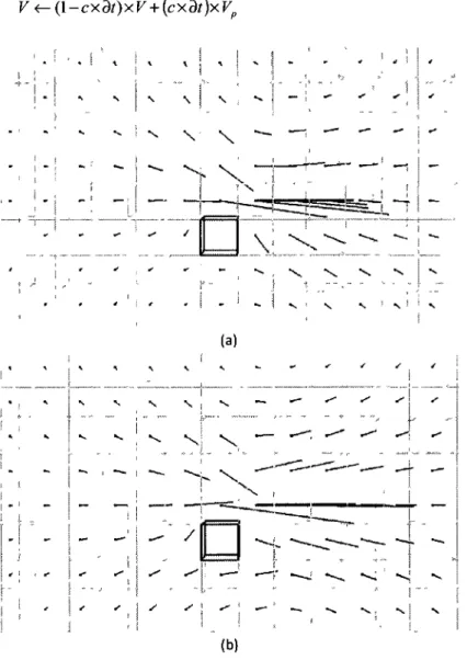
With full calculation, an obstacle like the black box shown m the Figure 2 requires us to
recalculate all quantities (velocities and pressure) in the fluid domain at each time step The
presence of an obstacle in the fluid domain entails a distortion m the velocity field We simplify
the full solver by not computing lines 4 to 11 in Pseudo-code 1 and by setting the number of
iterations for the null divergence step In fact, the divergence minimization process from lines 16
to 29 is m some cases performed more than 10 times when we set s_f E p s i l o n = 0 0001 In
the case of the "obstacle heunstic" we set the number of iterations around 2 to make the process
faster
The new velocity is computed by the interpolation described below Let V be the current velocity
on a face, Vp and the precomputed velocity on the same face, c is a constant that is set to
determine how fast the velocity field is returned to the precomputed state when an obstacle is
removed dt is the time step The interpolation is done by Equation 4
V<-(l-cxdt)xV + (cxdt)xV
Equation 4 i\.
•* N . „ . V N • ^ i>L
V
.
" > \
. —
/
^
,
' >,
(b)Figure 2 Images of the velocity field (a) from the full solver, (b) form the obstacle heuristic
The computation of a null divergence field allows velocity modification around the obstacle
Null divergence means that the fluid flowing in equals the fluid flowing out In fact, the
velocities on the faces of the obstacle are zero, so the null divergence ensures that the fluid on
the neighbonng voxels gets around the obstacle
The "obstacle heunstic" steps are summarized m Listing 0 2
12Listing 0 2 Pseudo-code of the obstacle heuristic
1 SimulateObstacleHeuristic(const float& deltaT) 2 {
3 // Update Velocities using the Precomputation 4 // for each face of each voxel
5 FaceVelocity = (1 OF - cstObstacle * deltaT) * FaceVelocity 6 + (cstObstacle * deltaT) * PreCompFaceVelocity,
7
8 // Null divergence step in Precomputed Version 9 PreCompDivergence(deltaT),
10
11 // Compute Voxel velocities by averaging
12 ComputeVoxelVelocities(), |
13 } j
The main advantage of using the "obstacle heunstic" is that we are able to add and move objects
in the fluid domain, starting from the precomputed velocity field without any obstacle The
results obtained with the heuristic (see Figure 2-(b)) are similar to those of the full Navier-Stokes
solver (see Figure 2-(a)), with the advantage that the process is at least twice as fast
Blower heuristic
In the fluid simulation, any change m the blower velocity direction means all quantities
(velocities and pressure) need to be recalculated m the fluid domain at each time step We
simplify the full solver to be able to simulate a dynamic blower
By observing fluid simulation and changes in velocity, we notice that the velocity is linear with
the norm of the blower velocity This means that if we double the velocity for the blower, the
resultant velocities on the other voxels are also doubled We also notice that when the blower
changes direction, each velocity of a voxel changes direction To be able to simulate the same
effect, we use precomputed velocities by aiming the blower in each direction corresponding to
the axes in the Cartesian coordinate system in the positive and negative directions In this article,
we use blower directions in 2 dimensions along the x and y axes, but we think the method can be
generalized to 3D We have to precompute the velocity field for the blower in directions (1 0,
0 0, 0 0), (-1 0, 0 0, 0 0), (0 0, 1 0, 0 0) and (0 0, -1 0, 0 0) Let 6 be the angle between the new
blower direction and the vector (1 0, 0 0, 0 0) For 6 between 61 and 62 we proceed as follows
• We identify 61 and 62 according to 6 For example 61 =0 and 62 =90 if 6 is between 0
and 90 degrees
• We compute the interpolation weight /Factor = (6 - 6l)/(Ô2 - 6l)
• Vpl the precomputed face velocities for 61
• Vp2 the precomputed face velocities for 62
• Each face velocity Fis computed by V= (1 0-/Factor)* Vpl +/Factor* Vp2
This heunstic is an approximation of the velocities yielded by the full solver version Figure 3
shows a comparison of velocities from the "blower heuristic" and the full solver The simulation
using the heunstic is more than twice as fast as the full solver
""" """•'7/ i '"
-/ -/ -/ I l i ,
y / / t 1 t s *• 1 I (a) (b) Figure 3 Images of the velocity field (a) from the full solver, (b) form the blower heuristicResults and Discussion
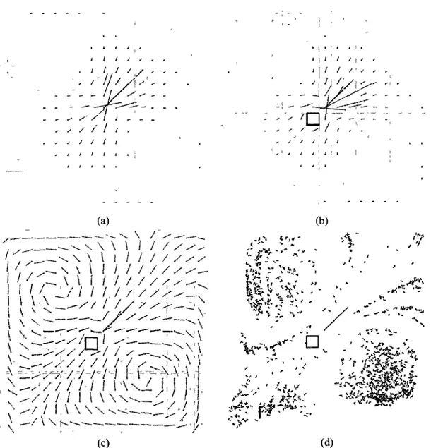
To visualize the fluid velocity field, the velocities on voxels can be displayed as vectors In this
case each velocity is represented by a vector We also able to visualize the velocity field with
unitary vectors for the direction and colors for the amplitude For example, the velocity can be
depicted in blue for a high amplitude or red for a low amplitude It is also possible to visualize
the velocity field with particles moving in the fluid domam The Figure 4 shows examples of
visualization methods
To illustrate how the heunstics work, we provide an implementation with the article The
program is written in C++ and uses OpenGL to display the 3D scene The user must set the
resolution of the fluid domain in terms of number of voxels In the case of Figure 4, the fluid
domain has 17x17x17 voxels and the blower (in blue) is at the voxel (8, 8, 8) We notice that the
14
gnd in Figure 4 represents all voxels with z = 8 in the fluid domam In fact it is not easy to
visualize the velocities with vectors when all 17x17x17 voxels are displayed
The full solver frame rate is around 172fps on a laptop equipped with an Intel CPU T2400 at
1 83GHz (dual core), with no parallelism in the simulation and visualization processes The same
scene usmg "blower heunstic" (see Figure 4-(a)) allows a frame rate around 392fps We get
331fps with the two heuristics (see Figure 4-(b))
Some other optimizations are possible in a game physics context For example, we don't have to
update the velocity field when the blower doesn't change and the obstacle doesn't move for a
certain time The heunstics of this article can be simply added to an existing game physics
engine The velocities can be precomputed at setup or loaded from a file
References
[1] R Bndson (2008) Fluid Simulation far Computer Graphics, A K Peters
[2] N Foster and D Metaxas (1996) "Realistic animation of liquids", Graphical Models and Image
Processing, 58(5) 471^t83
[3] Harlow, F H , and Welch, J E (1965) "Numencal calculation of time-dependent viscous incompressible flow," Phys Fluids, 8 2182-2189
[4] L Quartapelle Numerical solution o/the incompressible Navier-Stokes equations Spnnger 1993
/ / /
•il'A
y.
_ / ,
,
/ 1 , .
/ / i t / t i t *(a) (b)
\ , y^—^\ \ \ I / / / / /
SS
[', , ^ \ \ \ I / / / / / / /
-(<-% \ \ I / / / « / / / / ^
(/ _// / u /*/s>^sr
I \^^
w
cR -f
:
—-"v\
V ^ / / / / / / / ' / . / ^>> \ t
=\ "i_>^ -y-?'-/,
=/ -/- / "-/ hi 1^*7" r> -7 7
- . V / / / I I IAN_/ J, .
. w / t,\ \ \ \ - * , ^ — » _ £ - ' ,-.
. \ ~-/\\s^~ -.. . dl.h
(c) (d)
Figure 4 Images of the velocity field visualization using heuristics (a) with vectors without an obstacle, (b) with vectors with an obstacle, (c) with unity vectors for the direction and color for the amplitude with an obstacle, (d) with an obstacle and particles
\
Chapitre 2
Visualisation d'écoulement d'un fluide
sur un maillage basée sur des particules
Résumé
Cet article présente une nouvelle méthode d'animation de particules sur un
maillage arbitraire triangulaire à partir d'un champ de vitesses de l'écoulement
d'un fluide La visualisation d'un champ de vitesses avec des particules permet
de produire de nouveaux effets spéciaux Une contrainte d'attraction est mise en
place pour corriger la vitesse d'une particule pour que sa trajectoire reste près de
la surface Une contrainte de répulsion est également utilisée pour assurer une
meilleure répartition des particules sur la surface Le champ de vitesses est
cal-culé à l'aide d'heuristiques basées sur la physique mis en oeuvre via un modèle
de chaînes Notre méthode est robuste et donne de bons résultats, en particulier
pour les simulations interactives, même pour les systèmes avec plusieurs milliers
de particules
Commentaires
Cet article porte sur la visualisation d'un champ de vitesses d'un fluide sur une
surface arbitraire Contrairement au premier chapitre dans lequel le champ de
vitesses est calculé dans une grille régulière 3D, ici le champ de vitesses est
C H A P I T R E 2 VISUALISATION D ' É C O U L E M E N T D ' U N FLUIDE
calculé sur un maillage triangulaire d'une surface Une fois le champ de vitesses
obtenu, nous y déposons des particules afin de créer des effets spéciaux de liquide
ou de fumée sur la surface de l'objet La visualisation par plusieurs milliers de
particules du champ de vitesses se fait en temps interactif, mais le rendu des
effets spéciaux pour la fumée ou pour l'eau prend plusieurs dizaines de secondes
par image Cet article a été présenté à 6th International Conference on Computer
Graphics, Virtual Reality, Visualisation and Interaction in Africa et publié dans
l'acte de conférence
Dans cet article, nous voulons obtenir un champ de vitesses sur un maillage
simulant la dynamique des fluides Pour obtenir le champ de vitesses, nous
uti-lisons des heuristiques décrivant la dynamique des fluides sur un maillage
trian-gulaire Ces heunstiques ont été introduites par Egh et Stewart [4] et utilisées
comme applications dans un cadre de programmation unifié d'une méthode
utili-sant le modèle des chaînes Dans [4], le champ de vitesses est calculé uniquement
sur une surface plane (en 2D) Nous avons modifié ces heunstiques pour une
sur-face à topologie arbitraire Cet article est également une suite de la méthode 2D
proposée dans [4]
Les contributions sont d'abord l'extension du générateur du champ de
vi-tesses d'une surface 2D à une surface à topologie arbitraire Ensuite, il y a la
génération d'effets spéciaux de fluide (avec la fumée et les liquides) sur une
sur-face par une méthode de visualisation du champ de vitesses avec des particules
Contrairement à tous les travaux ayant abordé la simulation de fluide sur une
surface, la méthode que nous proposons est la première à utiliser les particules
afin de visualiser le fluide Les résultats obtenus permettent de conclure que la
résolution du maillage de la surface ne semble pas beaucoup influencer la
visua-lisation du champ de vitesses II est aussi important de noter que les distances
géodésiques entre les sommets des tnangles du maillage de la surface pourraient
être pré-calculées pour la contrainte de répulsion entre les particules Mais il est
possible que cela n'ait pas un impact majeur sur la qualité du résultat final L'idée
de la simulation de fluide sur une surface avec des particules a été proposée par
le professeur Richard Egh J'ai implémenté le code, validé la méthode proposée
et rédigé l'article sous sa supervision
Particle-based Fluid Flow Visualization on Meshes
Khahd Djado * Richard Egh + Centre MOIVRE, Département d'Informatique Université de Sherbrooke, Sherbrooke, Québec, CANADA
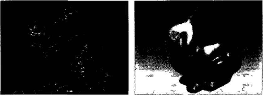
Figure 1 Fluid on the Bunny s surface liquid and smoke
Abstract
This paper presents a new method for animating particles on an arbitrary triangular mesh starting from a fluid flow velocity field The velocity field visualization with particles allows the produc-tion of new special effects An attracproduc-tion constraint is introduced to correct a particle s velocity so that its trajectory remains near the surface A repulsion constraint is also used to ensure a better distn bution of particles on the surface Our velocity field is obtained by physically-based heunstics implemented using a chain model Our method is robust and yields good results, in particular for interactive simulations, even for systems with several thousand particles CR Categories 13 7 [Computer Graphics] Three-Dimensional Graphics and Realism—Animation
Keywords fluid animation, flow on surface particles velocity field, visualization
1 Introduction
Fluid animation methods generally consist of two parts the simu-lation model that governs the movement of the fluid and the visu-alization of the created velocity field Simulation models fall into two broad categones those using Eulenan grids and those using Lagrangian particles For visualization, there are two popular ap-proaches texture deformation or synthesis and the particle system In this paper, we visualize a fluid flow velocity field (created on a triangular grid by a Eulenan method) with particles
The first work on animation of a fluid on a surface was done by Stam [Stam 2003] followed by Shi and Yu [Shi and Yu 2004] The
* Khahd Djado@USherbrooke ca t Richard Egh@USherbrooke ca
simulation model in [Stam 2003] is an extension of a 2D Navier Stokes fluid solver to curvilinear coordinates over Catmull-Clark surfaces, by using global surface parametnzation In [Shi and Yu 2004], the simulation model is built directly on the mesh space for inviscid and incompressible flow Fan et al [Fan et al 2005] also tackled fluid simulation on a surface by using an unstructured Lattice Boltzmann Model (LBM) from 2D meshes to 3D surface meshes Lui et al [Lui et al 2005] present a method for solv ing Navier-Stokes equations on manifolds using a global conformai parametnzation Recently Elcott et al [Elcott et al 2007] used an arbitrary simplicial mesh to define a fluid domam and simulate a fluid on a surface by using differential forms to solve the Navier-Stokes equations All of these methods use texture deformation or synthesis to visualize the velocity field on the surface
A common way to visualize a velocity field is by deforming or syn thesizmg a texture under the effect of the field [van Wijk 2002, Weiskopf et al 2003, Li et al 2003, Laramee et al 2004, Weiskopf and Ertl 2004, Li et al 2008] Flow visualization with particles has been the subject of much work, including [Bauer et al 2002 Kruger et al 2005] Certain authors have considered 3D flow visualization near a surface [van Wijk 1993, Max et al 1994] These studies [Bauer et al 2002, Kruger et al 2005 van Wijk 1993, Max et al 1994] have been pnmanly interested in the interaction between par-ticles and the surface of an object in the velocity field The object is an obstacle in the 3D velocity field The specific case of flow-on-surface visualization using particles has not been explored The pnncipal contnbution of this paper is to visualize fluid flow on sur-face with particles
Particles are commonly used in computer animation The mam rea-son for using a particle system for velocity field visualization is to obtain other classes of special effects for fluid flow on a surface which are difficult to realize with texture deformation or synthe-sis (see Figure 1) Our visualization method with a particle sys-tem uses a simple velocity interpolation technique and an attraction constraint to keep the particles near the surface We also use a re-pulsion, as in [Witkin and Heckbert 1994] but for arbitrary meshes, to ensure a better distnbution of particles on the surface
Like the studies descnbed in [Shi and Yu 2004 Fan et al 2005, Elcott et al 2007] our method works directly on an arbitrary mesh Our velocity field is obtained by very simple
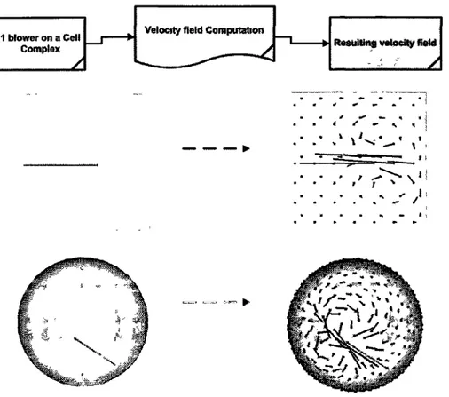
1 blower on a Cell Complex
à
Velocity field Computation
Resulting velocity field
^_-
ê
Figure 2 Summary of the velocity field computation Form left to nght we first add a blower in red (fluid velocity source), then we compute the velocity field by simulation The result of the simulation is a 2-chain (velocities inside 2-cells)
based heuristics But the particle-based visualization method pro-posed m this paper can work with any velocity field on arbitrary meshes using other fluid simulation techniques The physically-based heunstics used here are an extension of a 2D fluid simula-tion work descnbed in [Egli and Stewart 2004] We modify these heunstics for an arbitrary surface in 3D The 2D simulation method in [Egli and Stewart 2004] is written in a high-level topological and algebraic data structure we have called C3 (Chain and Cell Com-plexes) We use the same C3 formulation C3 is defined with the aim of finding neighbor and adjacency information easily In fact, the management of a transferred fluid mass from a tnangle to its neighbors is very simple to wnte in the C3 formalism
In this paper we propose a new approach to animate a fluid on a surface with arbitrary topology Our specific contnbutions are • a visualization of a flow on a surface using particles, in contrast to all related work m computer animation [Stam 2003 Shi and Yu 2004, Fan et al 2005, Lui et al 2005, Elcott et al 2007], • an attraction constraint toward the surface and a repulsion be-tween particles in the context of a flow on surface
» other classes of special effects such as volumetric smoke and
liq-uid flows,
The rest of this paper is organized as follows in section 2, we give a basic overview of the C3 formulation, with some definitions and a summary of the velocity field computation process by simulation
Section 3 describes the velocity field visualization method Then we give our results with some details on the implementation in sec-tion 4 Secsec-tion 5 presents our conclusion
2 Fluid Velocity Field
2 1 Basic Overview of C3
In computer graphics, the implementation of a surface subdivision program like the Catmull Clark surface subdivision [Catmull and Clark 1978] or mesh simplification [Hoppe 1996] requires informa-tion on the neighbor and adjacency relainforma-tionships between tnangles edges and vertices The cell complex concept was developed as a way of finding neighbor and adjacency information easily A cell complex is the descnption of a system in tenus of cells of differ-ent dimensions For example a surface mesh of a 3D object is a 2-complex and the 0-cells, 1 -cells and 2-cells are respectively, the vertices edges and faces of the polygons (0-cell = vertex 1-cell = edge and 2-cell = face) The concept of chain is used to manipulate quantities on a cell complex
A p-chain is defined over a cell complex and assigns a coefficient to each p-cell in this cell complex For example the fluid mass on each 2-cell can be stored in a 2-chain of reals In certain applications coefficients may be associated with cells of different dimensions A complete fluid ammation on a plane based on heunstics and
plemented in C3 formulation is presented in [Egli 2000, Egli and Stewart 2000b, Egli and Stewart 2004] We use the same frame-work and its application programming interface (API) here More details about the C3 framework and its API can be found in [Egli and Stewart 2000b, Egli and Stewart 2000a, Egli 2000, Egli and Stewart 2004]
One of the major advantages of chains is their use for the descnp-tion of models We first define and initialize all chains which can be used in the simulaUon model Formulas and laws are then applied directly to the chains This allows for global, unified treatment of the cell complex, simply as a transfer between cells inside the com-plex (fluid mass for example) The implementation of a fluid flow on an arbitrary surface becomes very simple by using the C3 API
2 2 Velocity Field Computation
The velocity field used in this paper is obtained by a fluid simula-tion on the cell complex At first we place flow sources (velocity sources) on selected 2-cells that we call the blower For example in the left image of Figure 2, we place only one blower, then we simulate the fluid after few time by using heunstics (four pnnciples that we call the Neighbour, Pressure, Friction and Border m the Appendix) Figure 2 shows the steps of the velocity field compu-tation process More details about these heunstics are presented in the Appendix section The result of the simulation is a 2-cham of the average velocity inside the cell complex
The goal of this paper is to visualize a fluid flow on surface with particles The input of our visualization method is a velocity field This velocity field can be obtained by the method descnbed in the appendix or other fluid simulation method
3 Fluid Visualization Method
In flow-on-surface visualization with textures it is sufficient to know the velocity of the fluid anywhere on the surface An in-terpolation from the velocities on 0-cells allows one to obtain the fluid velocity anywhere inside a 2-cell In the case of particles it should be noted that they do not necessanly remain on the surface Without any attraction, we note that the particles will eventually get away from the surface This is more obvious when the parti-cle s velocity is large and when the partiparti-cle is located in places with high curvature of the surface We use an attraction-like constraint to keep particles near the surface Once we ensure that the particles remain near the surface we see that after some time the particles concentrate in certain areas like in area with low velocity field (see Figure 6(c)) To prevent this we use repulsion between particles
31 Particle Velocity Interpolation
Our velocity field is summanzed by the average fluid velocity on each 2-cell on the surface (cell complex), stored in the 2-cham
ch2.va But we need the velocities on the 0-cells for the
inter-polation of each particle's velocity These velocities on the 0-cells are computed in a 0-chain chOjva We note that velocity averaging starting from ch2jva and moving to ch0-va is not a valid approach For example as shown in Figure 3(a) we obtain a velocity near zero by using ( K + Vb)/2 This problem is mentioned m [Shi and Yu 2004] The solution proposed in [Shi and Yu 2004] is to apply a local flattening, achieved by parametenzations Rather than this solution, we use a simpler approach by interpolating the velocity directions and velocity norms separately Although this is not justi-fied mathematically, we obtain good results with this approach (see Figure 3(b)) Since we have the velocities on the 0-cells, they are used to compute the velocity of each particle by interpolation
Figure 3 The velocity on a 0-cell (1 and 2) (a) by averaging veloc-ities on 2-cells (a and b), (b) by averaging velocity directions and averaging velocity norms on the same 2-cells (a and b)
Let P be a particle position on the 2-cell ABC of Figure 4 The velocity Vt at point P at time t is determined by a quasi-barycentnc velocity interpolation VA VB and Vc with weights (SA/(SA +
SB + Sc)) for vertex A (SB/(SA + SB + Sc)) for vertex B
and (SC/(SA + SB + Sc)) for vertex C SA, SB and Sc are the areas of the three tnangles of the tetrahedron PABC, as shown in Figure 4 We used quasi quasi-barycentnc velocity interpolation because the projection of P on 2-cell ABC is not always inside of it, so barycentnc couldn't be used Now, we just need to find the 2-cell associated with each particle
Figure 4 Velocity interpolation method for a particle at position P above the 2-cell composed of the A, B and C vertices
Each particle is associated with a 2-cell at each time step This localization of the nearest 2-cell to a particle is a problem similar to collision detection We must find the index of the 2-cell nearest to the particle at each time step To find this index, we use a Proximity
Query Package (PQP) [Gottschalk et al 1996, Larsen et al 1 The index returned by the PQP is updated in the particle attnbutes The velocity of the particle is interpolated from the velocities of 0-cells which constitute the returned 2-cell
3 2 Attraction Constraint
Let M be the middle point of the 2-cell shown in Figure 4 and TV the normal vector of the 2-cell An attraction-like constraint is used to conect each particle's velocity Let Ka be the attraction factor For the particle P in Figure 4 the attraction is given by
jtt = -Ka*{Mp N) N (1) The distance between each particle and the 2-cell is given by (MP
N) The particle velocity is changed by adding the attraction term At The (MP jv ) value changes sign depending on whether the
particle is above or below the point M The new particle velocity is expressed by Vt <— Vt + At
We allow the user to control the proximity of the particles to the surface via the constant parameter Ka and another constant param-eter Km Km moves point M along the normal vector to the 2-cell
In this way particles can be kept closer or farther to the surface
3 3 Repulsion Technique
For repulsion we use a Gaussian function of the type descnbed in [Witkin and Heckbert 1994] The repulsion of particle i on particle
j at respective positions P, and P} is expressed by
• a. e x p ( -HÎV^ii ) x
HHKH (2)
In Equation 2 a is an attenuation factor for the repulsion between particles and a is the standard deviation making it possible to con-trol the distnbution of particles On the surface of a 3D object, it is more appropnate to use the geodesic distance rather than Euclidian distance to compute the repulsion between particles i and j But for reasons of performance and complexity, we use Euclidian distance between particles in a same area The obtained results are stable An index of a 2-cell is associated with each particle Starting from this index, we use C3 to find 2-cells around a particle It is thus easy starting from a given particle i to find all particles j close to it (within a radius r) on the 2-cells around it The user specifies the size of the neighborhood by indicating the number of implied neighbors n and the radius r For example, n is 1 for the 2-cells neighbors to the cunent 2-cell n is 2 for the neighbors of the neigh-bors (including 2-cells for n — 1) The repulsion depends on the distance of the nearby particles For each particle i the repulsion is expressed as a velocity conection Vt *- Vt — Yl £s ^«J- w n e r e
S% is a set of particles around % according to r and n In this way particles are better distnbuted on the surface
2-chain ch2jva Steps 8 to 14 contain the particle-based velocity field visualization process Step 8 finds the fluid velocity for each 0-cell of the complex in the 0-chain chQjva The velocity field is obtained starting from this 0-chain After step 14 we display the result particles move on the surface according to the velocity field
1 Load the 3D object mesh,
2 Build the cell complex o-ceiis 1 -ceils
2-cells, border and cell relationships,
3 Initialize chains, number of particles, Ka,
Km, alpha and sigma
*
V
4 Neighbour principle, 5 Pressure principle, 6 Friction pnnciple, 7 Border pnnciple,( 8 Compute velocities at 0-cells )
Static velocity
field
For each particle
9 Return 2-cell index near the current particle using PQP,
10 Use 3 velocities on 0-cells from the returned 2-cell index to compute the current particle velocity by barycentnc Interpolation,
11 Compute repulsion between the current particle and particles around it, 12 Correct the current particle's velocity to
keep it near the surface,
Update the current particle velocity, Update the current particle position
13 14
V _
Display
Figure 5 Summary of our flow model
We use two approaches in our flow method depending on whether the velocity field is static or dynamic In the static case, we fix the number of blowers, and we compute the velocity field dunng few time in order to allow the expansion of the fluid over the entire surface Then we carry out the velocity field visualization process The static approach saves a lot of time, because the velocity field resulting from the simulation model is pre calculated in the 0-chain
chOjva In the dynamic case the blowers are dynamic so the steps
from 4 to the display are repeated at each time step
4 Results and Discussion
4 1 Summary of the Animation Method
Our complete flow method (simulation and visualization) is sum-manzed by the diagram in Figure 5 Steps 1 to 3 are for the con-struction and initialization of C3 Steps 4 to 7 compnse the simu-lation process and return the average velocity on each 2-cell in the
4 2 Experimental Results
Our flow model has been tested on a sphere, a brezel model (from Javaview) and the Stanford bunny The code is implemented in C++, using OpenGL for the rendenng, and our program runs on a laptop equipped with an ATI Mobility Radeon XI300 graphics card and an Intel CPU T2400 at 1 83GHz (dual core), with no par-allelism in the simulation and the visualization process
As opposed to texture, particles offer the possibility of different effects such as smoke and liquid flows For instance, with particles it is possible to produce
• real-time fire or smoke by using spntes, • liquids by using implicit surfaces
• volumetric smoke by using volumetnc spheres
We present two examples of special effects produced by our flow visualization method a liquid and a volumetnc smoke (using vol-umetnc spheres) Some images resultmg from animation of the tested models are given in Figure 1 Figure 6 illustrates the move-ment of the particles more clearly, as they are represented by small black spheres These results are for a static velocity field built after 400 time steps (where one time step = 0 005) The tested mod-els contain 362 vertices (0-cells) and 720 tnangles (2-cells) for the sphere 958 and 1920 for the brezel and 793 and 1561 for the bunny To use our application, the users set blowers on selected 2-cells After the velocity field is computed particles are launched on the surface At t = 0, particles can be randomly placed on the surface as shown in Figure 6 (a), or placed on a selected 2-cell as in Figure 6 (f)
For the images in Figure 6 (0, (g) and (h), 500 particles are placed on one 2-cell on the bunny model This yields the volumetnc smoke effects shown in nght image of Figure 1 To obtain this effect we initialize a = 0 0 then set a = a + 0 005 at each time step for a few seconds This avoids a strong repulsion of particles For the brezel model in Figure 6 (l) (j) a r |d (k), 3000 particles are used
In Figure 6 (a) 3000 particles are randomly placed on the sphere with null velocity field Using repulsion alone, we obtain the image in Figure 6 (b) after a few frames In Figure 6 (c), we compute a velocity field with 3 blowers and no repulsion The particles are grouped together after a few seconds In Figure 6 (d) we add a slight repulsion and in Figure 6 (e) we use more repulsion The frame rate for the sphere with 1000 particles is 31 fps For the brezel and the bunny with 1000 particles we obtain 22 fps and 32 fps, respectively For the same sphere with 3000 particles, we ob-tain 5 fps and 0 9 fps with 10000 particles In the case of a dynamic velocity field each blower has random direction and magnitude Thus the velocity field changes at each time step We apply a dy-namic velocity field to the bunny with 1000 particles and the frame rate is 5 fps
We use data from particle positions to render liquid and volumetnc smoke effects For the liquid, we use a blobby system to produce implicit surfaces and the results are produced by a ray tracing with reflective and refractive matenals (see left image of Figure 1) The rendenng time for the tested models varies from around 1 minute to 4 minutes per image For the smoke we use spheres with trans-parency, and noised and animated textures (nght image of Figure 1 ) The rendering time is around 3 to 7 minutes per image The Fig-ure 7 shows smoke and liquid effects on the sphere
The particle s velocity modified by the attraction and the repulsion constraints can cause a certain distortion of visualization compared to the methods of scientific visualization using textures, for exam-ple This distortion is more important when there is high repulsion between particles Our velocity field visualization method with par-ticles is not necessanly intended for scientific purposes, but rather for special effects in computer ammation The attraction and repul-sion allow the user (an artist) to produce the effects he wants
5 Conclusion
In this paper, we have presented a new approach for animating particles on an arbitrary triangular mesh Unlike previous meth-ods which simulate fluid flow on surfaces we use particles instead of texture to visualize the velocity field We add a repulsion be-tween particles and an attraction on the surface Our method allows the production of new classes of special effects such as liquid and smoke flows Our approach uses no parametnzation m either the simulation or the visualization process
Acknowledgements
This research was supported in part by grants from the Natural Sciences and Engmeenng Research Council of Canada The au-thors would like to thank Jean François Le Fillâtre Gilles-Philippe Paille Piene-Marc Jodoin Lon Krung and Chnstian Preciado Castelo for their comments
References
BAUER D , PEIKERT, R , SATO M AND SICK M 2002 A
case study in selective visualization of unsteady 3d flow In VIS
02 Proceedings of the conference on Visualization 02 IEEE
Computer Society, Washington DC, USA 525-528
CATMULL E , AND CLARK, J 1978 Recursively generated
B-spline surfaces on arbitrary topological meshes Computer Aided
Design 10 (Sept ), 350-355
EGLI R AND STEWART N F 2000 A framework for system specification using chains on cell complexes Computer-Aided
Design 32 447-459
EGLI R , AND STEWART, N F 2000 Graphical simulation using chain models In Technical Report 1174 Département informa
tique et de recherche opratwnnelle Université de Montreal July
EGLI R , AND STEWART N F 2004 Cham models in computer simulation Math Comput Simul 66 6 449-468
EGLI R 2000 Cadre de travail pour la specification de systèmes avec des chaînes sur un complexe cellulaire Phd thesis, Départe-ment informatique et de recherche oprationnelle, Université de Montreal, May
ELCOTT, S , TONG, Y , K A N S O E , SCHRODER P , AND D E S
-BRUN, M 2007 Stable, circulation-preserving, simplicial flu-ids ACM Trans Graph 26, 1 4
FAN, Z ZHAO, Y , KAUFMAN, A , AND H E Y 2005 Adapted
unstructured lbm for flow simulation on curved surfaces In SCA
05 Proceedings of the 2005 ACM SIGGRAPH/Eurographws symposium on Computer animation, 245-254
FOSTER N , AND METAXAS, D 1996 Realistic animation of liq-uids In GI 96 Proceedings of the conference on Graphics in
terface 96 Canadian Information Processing Society Toronto
Ont, Canada, Canada 204-212
GOTTSCHALK, S , LIN, M C , AND MANOCHA, D 1996
Obb-tree a hierarchical structure for rapid interference detection In
SIGGRAPH 96 Proceedings of the 23rd annual conference on Computer graphics and interactive techniques 171-180
HOPPE, H 1996 Progressive meshes In SIGGRAPH 96 Pro
ceedings of the 23rd annual conference on Computer graphics and interactive techniques, 99-108
K R U G E R , J , K I P F E R , P , K O N D R A T I E V A , P , A N D W E S T E R
-MANN, R 2005 A particle system for interactive visuahzaUon of 3d flows IEEE Transactions on Visualization and Computer
Graphics 11 6 7 4 4 - 7 5 6
L A R A M E E , R S , H A U S E R , H D O L E I S C H H , V R O L I J K , B ,
P O S T F H , A N D W E I S K O P F D 2004 The state of the art in flow visualization Dense and texture-based techniques Com
puter Graphics Forum 23 2004
L A R S E N , E , G O T T S C H A L K , S L I N , M C , A N D M A N O C H A , D
Fast proximity q u e n e s with swept sphere volumes In Technical
report TR99-018 Department of Computer Science University ofN Carolina Chapel Hill
L i , G -S , B O R D O L O I , U D , A N D S H E N , H - W 2003
Chameleon An interactive texture-based rendenng framework for visualizing three-dimensional vector fields In VIS '03 Pro
ceedings of the 14th IEEE Visualization 2003 (VIS 03), 32
L i , G - S , T R I C O C H E , X , W E I S K O P F , D , A N D H A N S E N , C D
2008 H o w charts Visualization of vector fields on arbitrary sur-faces IEEE Transactions on Visualization and Computer Graph
ics 14, 5, 1067-1080
L U I , L , W A N G , Y , A N D C H A N T F 2005 Solving pdes on man-ifold using global conformai parametenzation In Variational
Geometric and Level Set Methods in Computer Vision Third International Workshop VLSM 2005 3 0 7 - 3 1 9
M A X , N C R A W F I S R A N D G R A N T C 1994 Visualizing 3d
velocity fields near contour surfaces In VIS 94 Proceedings
of the conference on Visualization 94, IEEE Computer Society
Press, Los Alamitos, C A U S A 248-255
S H I , L A N D Y U , Y 2004 Inviscid and incompressible fluid simulation on tnangle meshes Comput Animât Virtual Worlds
15 3-4 173-181
S T A M , J 2003 Flows on surfaces of arbitrary topology In SIG
GRAPH 03 ACM SIGGRAPH 2003 Papers IIA-IIX
VAN WIJK, J J 1993 Flow visualization with surface particles
IEEE Comput Graph Appl 7 3 , 4 , 1 8 - 2 4
VAN W I J K , J J 2002 Image based flow visualization In SIG
GRAPH 02 Proceedings of the 29th annual conference on Computer graphics and interactive techniques 7 4 5 - 7 5 4
W E I S K O P F , D , A N D E R T L T 2004 A hybnd physical/device-space approach for spatio-temporally coherent interactive tex-ture advection on curved surfaces In GI 04 Proceedings of
Graphics Interface 2004, Canadian Human-Computer
Commu-nications Society School of Computer Science University of Waterloo, Waterloo, Ontano, Canada, 2 6 3 - 2 7 0
W E I S K O P F , D , E R L E B A C H E R G , A N D E R T L T 2 0 0 3 A
texture-based framework for spacetime-coherent visualization of time-dependent vector fields In VIS 03 Proceedings of the 14th
IEEE Visualization 2003 (VIS 03), 15
W I T K I N A P , A N D H E C K B E R T , P S 1994 Using particles to sample and control implicit surfaces In SIGGRAPH 94 Pro
ceedings of the 21st annual conference on Computer graphics and interactse techniques 269-211
6 Appendix
The velocity field used in this paper is obtained by a fluid simulation on the cell complex by based heunstics This physically-based heuristics, is an extension of a 2D fluid simulation work de-scnbed by Egli and Stewart in [Egli and Stewart 2000b, Egli and Stewart 2004] The 2D results produced are visually comparable to those of more classical methods based on the Navier-Stokes equa-tions [Foster and Metaxas 1996]
The simulation model is based on the model suggested by Egli and Stewart in which fluid advances on each 2-cell between time t and
t + dt according to four pnnciples that we call the Neighbour, Pres-sure, Friction and Border pnnciples
The quantities associated with each 2-cell at time t are the fluid mass m, the average velocity vt and the density p (p = m/s where s is the area of the 2-cell)
Neighbour principle The fluid mass in a 2-cell moves in the
direc-tion of the velocity vt, and part of it is transferred to neighbounng cells
Let m„out, be the outgoing fluid mass from the current 2 cell to its adjacent 2-cell i impelled by velocity vt Let m, be the initial fluid mass on the 2-cell i The fluid velocity UaX on the 2-cell i is computed as follows
m Vaz + mvout Va
(3)
The fluid masses are updated by m <— m — ] P mt o ut and
where kf is a fnction constant with 0 < kj < •£- (the value 0 conesponds to no fnction)
inter-cellular fnction
There is a similar effect related to
Border principle The direction of the average velocity vt within a
2-cell tends to follow the border of the object
The Border principle leads to a heunstic to ensure that the di-rections of the average velocities vt m each 2-cell touching the boundary of the geometnc object will have a tendency to follow the boundary Every 1-cell that has only one adjacent 2-cell forms part of the boundary of the object The conection applied, in order to implement our Border principle, is this
(1 - khAt)vt + kbAtvt (7)
Here fcj, is a constant that determines to what extent the velocity will have a tendency to follow the boundary (the higher the value of the constant, the larger the influence of the boundary on the veloc-ity but the value of the constant must satisfy 0 < fct At < 1), and
vt is the projection of the velocity vt on the boundary
vt = (vt I I " ^ ! ! ' (8)
where 1* is the difference between the geometnc positions of the 0-cells adjacent to the relevant 1-cell
The fluid simulation model using these four pnnciples as descnbed below, is only valid m the case of a planar tnangular mesh A complete descnptions of these principles are given in [Egli 2000, Egh and Stewart 2000b, Egli and Stewart 2004]
Pressure principle A part of the fluid mass in a 2-cell is displaced
towards neighbounng 2-cells with lower pressure
Let mp0utt, the outgoing fluid mass from the current 2-cell to its
adjacent 2-cell i due to the pressure difference Let Vp\ the velocity of the fluid mass acquired due to the pressure difference As in the Neighbour pnnciple the fluid mass velocity Uat on a 2-cell i is updated as follows
Extension to a 3D Surface
™iVai+™Po<Lt,Vpz
m,+mpout (4)
The fluid velocity vt on the current 2-cell changes according to
. mVa + } J "ipout.%
và< T¥*
m1+2^ "ipoutj
(5)
As in the Neighbour principle, the fluid masses on the cunent 2-cell and its neighbour 2-cell i are updated by m <— m — ^2 mpout,
and nil <— m, + mp0ut.
Fnction principle There is fnction between a 2-cell and its
neigh-bonng 2-cells, as well as internal fnction within a 2-cell We begin the calculations by using the updated values of the veloc-ities obtained by application of the first two pnnciples Due to the posited effect of internal fnction, the velocity vt of the fluid mass in a 2-cell decreases with time To model this phenomenon we use the following formula
Figure 8 Transfer of fluid direction from a 2-cell to an adjacent 2-cell
To extend the model to surfaces with an arbitrary tnangular mesh we mainly modify the Neighbour and Pressure pnnciples In the arbitrary surface case (mesh in 3D), the vectors m ^ o u i , ^ in Equation 3 and mp 0t i t , ^ t in Equation 5 in the TVeighbour and
Pressure pnnciples must be transfened to the appropnate planes
(2-cells are not necessanly in the same plane) To address this prob-lem, we add a rotation operator in the C3 API to make sure that the vectors are brought back onto the plane The Figure 8 illustrate the rotation of a vector from a 2-cell to an adjacent 2-cell
(l-kfAt)vt (6)