HAL Id: tel-02127058
https://pastel.archives-ouvertes.fr/tel-02127058
Submitted on 13 May 2019HAL is a multi-disciplinary open access archive for the deposit and dissemination of sci-entific research documents, whether they are pub-lished or not. The documents may come from teaching and research institutions in France or abroad, or from public or private research centers.
L’archive ouverte pluridisciplinaire HAL, est destinée au dépôt et à la diffusion de documents scientifiques de niveau recherche, publiés ou non, émanant des établissements d’enseignement et de recherche français ou étrangers, des laboratoires publics ou privés.
aortic valve tissues
Colin Laville
To cite this version:
Colin Laville. Mechanical characterization and numerical modeling of aortic valve tissues. Materials. Université Paris sciences et lettres, 2017. English. �NNT : 2017PSLEM069�. �tel-02127058�
de l’Université de recherche Paris Sciences et Lettres
PSL Research University
Préparée à MINES ParisTech
MECHANICAL CHARACTERIZATION AND NUMERICAL MODELING
OF AORTIC VALVE TISSUES
CARACTÉRISATION MÉCANIQUE ET MODÉLISATION NUMÉRIQUE
DES TISSUS DE VALVE AORTIQUE
École doctorale n
o364
SCIENCES FONDAMENTALES ET APPLIQUÉES
SPÉCIALITÉ MÉCANIQUE NUMÉRIQUE ET MATÉRIAUX
Soutenue par Colin Laville
le 13 septembre 2017
Dirigée par Yannick Tillier
COMPOSITION DU JURY :
M. Stéphane Avril
MINES Saint–Étienne, Président du jury Mme Valérie Deplano
Université Aix–Marseille II, Rapporteur M. Laurent Delannay
Université catholique de Louvain, Rapporteur M. François Bay
MINES ParisTech, Examinateur M. Yannick Tillier
CNRS UMR 7635
1 rue Claude Daunesse, CS 10207, 06904 Sophia Antipolis Cedex, France http://cemef.mines-paristech.fr
Mes premiers remerciements vont aux différents membres de mon jury qui ont accepté de relire et d’examiner mon travail. Je remercie Stéphane Avril d’avoir bien voulu présider ce jury. Un grand merci également aux rapporteurs, Valérie Deplano et Laurent De-lannay, ainsi qu’aux examinateurs, François Bay et Yannick Tillier, pour l’intérêt qu’ils ont manifesté et la discussion pertinente qu’ils ont su apporter à mes travaux. Je tiens tout particulièrement à remercier Yannick, mon directeur de thèse, pour m’avoir accordé sa confiance à travers une grande liberté de travail, mais aussi pour son soutien et sa disponibilité.
Je tiens ensuite à exprimer mes remerciements envers Christophe Pradille pour avoir rendu possible la réalisation de cette machine de traction indispensable à ma thèse, ainsi que pour ses conseils et son aide notamment en corrélation d’images et en analyse in-verse. J’aimerais également remercier les différents membres du groupe MEA, Christelle Combeaud pour s’être impliquée dans le développement de la machine, Francis Fournier pour en avoir réalisé la conception, Arnaud Pignolet pour le développement du logiciel de contrôle et Marc Bouyssou pour l’usinage des différentes pièces. Merci aussi à Sélim, Carole et Hallen du groupe SCS pour le temps qu’ils ont consacré à la résolution de mes problèmes informatiques, et à Thomas Olivier du laboratoire Hubert Curien à Saint– Étienne, pour m’avoir permis d’utiliser le microscope confocal et pour son aide précieuse lors de la campagne expérimentale. Je tiens également à remercier chaleureusement le personnel administratif du laboratoire, Marie–Françoise et Sylvie, toujours de bonne humeur et disponibles pour aider les étudiants.
Je me dois enfin de remercier mes collègues doctorants et post–doctorants sans qui ces années de thèse auraient été beaucoup moins enrichissantes. Merci à Florian et Daniel pour avoir patiemment répondu à mes questions parfois naïves, à Xavier pour avoir pris le temps de me guider dans la découverte du code source de FORGE®, à Modesar pour son aide très précieuse notamment en algorithmique, à mes collègues de bureau Fabien et Christophe pour nos discussions et le soutien mutuel, mais aussi à Ziad, Ali, Mehdi, Antoine, Luis, Romain, Grégoire, Pierrick, Abdel, Stéphanie, Benjamin, Danai et les autres. Un grand merci à tous pour les bons moments passés ensemble.
Pour finir, je voudrais remercier mes proches et tout particulièrement mes parents, pour leur soutien sans faille pendant toutes ces années.
General Introduction 1
1 Aortic valve tissues 7
1.1 Introduction . . . 8
1.2 Mechanical characterization . . . 11
1.2.1 Specimen preparation . . . 11
1.2.2 Biaxial device . . . 11
1.2.3 Digital image correlation method . . . 13
1.2.4 Experimental protocol . . . 13
1.3 Fibers orientation measurement . . . 15
1.3.1 Specimen preparation . . . 15
1.3.2 Confocal laser scanning microscopy and experimental setup . . . . 16
1.3.3 Experimental protocol . . . 17
1.4 Experimental results . . . 18
1.4.1 Biaxial tensile tests results and discussion . . . 18
1.4.2 Confocal laser scanning microscopy results and discussion . . . 29
1.5 Summary of Chapter 1 . . . 34
1.6 Résumé en français . . . 35
2 Mechanical framework and models 37 2.1 Introduction . . . 38
2.2 Continuum mechanical framework . . . 39
2.2.1 Kinematics . . . 39
2.2.2 Stress and objectivity . . . 43
2.2.3 Hyperelastic framework . . . 45
2.3 Lagrangian variational formulations of the problem . . . 48
2.3.1 Boundary conditions . . . 49
2.3.2 Weak formulation of balance equations . . . 50
2.3.3 Total Lagrangian formulation . . . 52
2.3.4 Updated Lagrangian formulation . . . 52
2.4 Finite element discretization . . . 56 2.4.1 Spatial discretization . . . 56 2.4.2 Temporal discretization . . . 62 2.5 Material models . . . 65 2.5.1 Fiber distribution . . . 65 2.5.2 Strain–energy functions . . . 68 2.5.3 Polyconvexity . . . 76 2.5.4 Fibers orientation . . . 76 2.6 Solver validation . . . 79
2.6.1 Convergence and stability . . . 79
2.6.2 Models implementation . . . 81
2.6.3 Fibers orientation algorithm . . . 85
2.7 Summary of Chapter 2 . . . 87
2.8 Résumé en français . . . 88
3 Inverse analysis procedure 89 3.1 Introduction . . . 90
3.2 Inverse analysis approach . . . 91
3.2.1 Generalities on inverse analysis . . . 91
3.2.2 Inverse analysis method . . . 93
3.2.3 Fibers dispersion and concentration parameters . . . 93
3.2.4 Numerical setup and inverse analysis procedure . . . 94
3.3 Inverse analysis results . . . 99
3.3.1 Models comparison . . . 99
3.3.2 Influence of input data . . . 101
3.3.3 Limitations of the inverse analysis procedure . . . 105
3.4 Summary of Chapter 3 . . . 105
3.5 Résumé en français . . . 106
4 Toward fluid–structure interaction 107 4.1 Introduction . . . 108
4.2 Governing equations . . . 109
4.2.1 Navier–Stokes equations for incompressible flows . . . 109
4.2.2 Boundary conditions . . . 110
4.3 SPH : method and implementation . . . 111
4.3.1 Generalities on SPH . . . 111
4.3.2 SPH interpolation . . . 112
4.3.3 First order differential operators . . . 114
4.3.4 Second order differential operator . . . 116
4.3.5 Accuracy of SPH differential operators . . . 116
4.3.7 Fluid discretization . . . 120
4.3.8 Incompressible SPH . . . 122
4.3.9 Boundary conditions treatment . . . 125
4.3.10 Time–stepping and numerical stability . . . 127
4.3.11 Reduction of the computational time . . . 127
4.4 SPH–FE coupling . . . 129
4.4.1 FSI algorithm . . . 129
4.4.2 Interface coupling . . . 130
4.5 Solver validation . . . 131
4.5.1 SPH implementation validation . . . 131
4.5.2 SPH–FE coupling validation . . . 134
4.6 Summary of Chapter 4 . . . 137
4.7 Résumé en français . . . 137
Conclusions and outlook 139 Appendix A Device protocol 143 A.1 Introduction . . . 143
A.2 Protocol . . . 143
Appendix B Material models derivatives 145 B.1 Introduction . . . 145
B.2 Weisbecker model . . . 145
B.3 Holzapfel Gasser Ogden model . . . 146
B.4 Modified Holzapfel Gasser Ogden model . . . 147
1 Heart circulation diagram . . . 2
2 Examples of prosthetic AVs . . . 3
3 AV replacement surgery with a mechanical prosthesis . . . 4
1.1 Microscopy images of some constituents . . . 8
1.2 Illustration of the AV displaying the leaflet structure . . . 9
1.3 Porcine AV leaflet excised . . . 11
1.4 The biaxial tensile device . . . 12
1.5 Example of subset tracking during deformation . . . 13
1.6 Sample mounted on the biaxial tensile devise . . . 14
1.7 Example of subset choice on 3D–VIC™ . . . 15
1.8 Confocal microscope Leica TCS SP2 SE form Hubert Curien Laboratory (Saint–Étienne, France) . . . 16
1.9 Optical system and objective . . . 17
1.10 Scheme of the observation areas positions (mm) on both samples . . . 17
1.11 Scheme of an excised AV leaflet . . . 18
1.12 Averaged thickness of the samples with dispersion for each valve . . . 19
1.13 (1 : 1) curves at be beginning and at the end of a complete loading protocol on a sample . . . 19
1.14 3D–DIC error measurement on an immersed plate submitted to a rigid body motion . . . 20
1.15 Example of nominal strain evolution function of the smoothing area for a subset size of 21 px . . . 21
1.16 Example of averaged strain on a frozen sample on three different areas . . 24
1.17 Example of averaged strain on a fresh sample on three different areas . . . 24
1.18 Tension–strain results for the (1 : 1) loading condition on six frozen sam-ples for both circumferential and radial axes . . . 25
1.19 Tension–strain results for the (1 : 1) loading condition on six fresh samples for both circumferential and radial axes . . . 25
1.20 Example of superposition of the tension–strain results for a representative frozen (blue) and fresh (red) sample using (1 : 1) loading condition . . . . 25
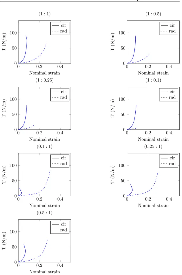
1.21 Tension curves on one representative frozen sample for the seven loading conditions of the experimental protocol . . . 26 1.22 Tension curves on one representative fresh sample for the seven loading
conditions of the experimental protocol . . . 27 1.23 Collagen fibers (channel 1) and elastin fibers and cells (channel 2) in the
arterialis . . . 30 1.24 Superposition of channel 1 and channel 2 . . . 30 1.25 Pictures of collagen fibers . . . 31 1.26 Four pictures of collagen fibers from a total stack of 140 µm depth . . . . 31 1.27 Illustration of angles measurements with respect to the picture frame . . . 32 1.28 Examples of principal orientation identification issues encountered while
processing confocal images . . . 32 1.29 Angles (°) interpolated on a real scale grid (mm) for the square sample . . 33 1.30 Angles (°) interpolated on a real scale grid (mm) for the whole leaflet . . 33
2.1 Lagrangian description of the motion . . . 40 2.2 Traction vectors acting on infinitesimal surface elements . . . 45 2.3 Illustration of the different types of boundary conditions . . . 49 2.4 P 1+/P 1 tetrahedron element with velocity (left) and pressure (right)
de-gree of freedom . . . 58 2.5 Decomposition of the P 1+/P 1 element into 4 sub–tetrahedrons . . . 59
2.6 Illustration of the Newton–Raphson algorithm where x0= xnis the initial (known) solution at t and xk = xn+1 is the converged solution at t + ∆t . 63 2.7 Characterization of the fiber direction vector in the tree–dimensional
Carte-sian coordinate system {E1, E2, E3} . . . 66
2.8 Examples of probability density functions ρr for 1 < λr< 1.5 . . . . 71 2.9 Relation between κ and b according to equation (2.135) . . . 74 2.10 Three–dimensional graphical representation of the collagen fibers
orienta-tion for several κ values . . . 74 2.11 Two–dimensional representation of the distribution ρ(θ) of the collagen
fibers for several κ values . . . 75 2.12 Illustration of the projection of a fiber direction (in red) from a 2D
mea-surement to a 3D geometry . . . 76 2.13 Illustration of the Djikstra’s algorithm on a 2D mesh to compute a
mini-mum distance d between the reference and current elements . . . . 77 2.14 Illustration of the projection method from a 3D geometry into a plane . . 78 2.15 Pressure applied on one–fourth of the geometry . . . 79 2.16 Pressure field in the quasi–incompressible case without and with stabilization 80 2.17 Pressure field in the incompressible case without and with stabilization . . 80 2.18 Evolution of the normalized volume with compression in incompressible
2.19 Isotropic models validation on uniaxial tension tests . . . 81 2.20 Circular fiber arrangement on one–eighth of a spherical balloon (arrows
indicate the orientation of the fibers) . . . 82 2.21 Inflation of the spherical balloon submitted to internal pressure with κ =
0.333, κ = 0.2 and κ = 0 from top to bottom (the norm of the displacement field kdk is shown) . . . 83 2.22 Energy conservation on a bending test (the norm of the displacement field
kdk is shown) . . . 84 2.23 Energy conservation during an indentation test on one–fourth of the
de-formable cube (the norm of the displacement field kdk is shown) . . . 85 2.24 Example of sinusoidal θ (°) interpolation and projection corresponding to
fiber orientation vectors . . . 85 2.25 Orientation projection on a complex 3D geometry of prosthetic valve (from
left to right : top, side and bottom views) . . . 86 2.26 Example of random κ interpolation and projection . . . 86 2.27 κ on a complex 3D geometry of prosthetic valve (from left to right : top,
side and bottom views) . . . 87
3.1 Evolutionary algorithm diagram . . . 92 3.2 Interpolation of measured fibers directions on the undeformed finite
ele-ment mesh . . . 94 3.3 Interpolation on the sample of the local concentration and dispersion
parameters . . . 95 3.4 Illustration of the modeled area at the initial and deformed states . . . 95 3.5 Scheme of an excised AV leaflet with radial and circumferential axes definition 96 3.6 Superposition of displacements from all the experimental loading
condi-tions on a representative fresh sample (DIC measurements) . . . 96 3.7 Superposition of forces from all the experimental loading conditions on a
representative fresh sample . . . 96 3.8 Displacements from DIC measurements imposed on the modeled geometry 97 3.9 Forces from experimental measurements to be compered to computed results 98 3.10 Forces from experimental (1 : 1) result (blue) and inverse analysis results
(red) for each model . . . 100 3.11 Forces from experimental (blue) and inverse analysis (red) results with
fixed angles . . . 102 3.12 Forces from experimental results (blue), 7 loadings identification (red),
5 loadings identification (green), 3 loadings identification (cyan) and 1 loading identification (magenta) . . . 103 3.13 Forces from experimental (blue) and inverse analysis (red) results with
3.14 Comparison of the experimental (blue) and numerical (red) tension curves
for a (1 : 1) loading condition . . . 105
4.1 Illustration of the different boundary conditions . . . 111
4.2 Example of bell–shaped function . . . 117
4.3 Neighbors of a particle i with its kernel support . . . 118
4.4 Plot of the non–normalized 5th order Wendland kernel and its derivative . 120 4.5 Illustration of three classic wall boundary conditions with from left to right : ghost particles, repulsive force and dynamic particles boundaries . 125 4.6 No–slip and free–slip wall boundary conditions from left to right . . . 126
4.7 Illustration of k–d tree algorithm functioning in 2D where li represents the splitting lines and pi the particles . . . 128
4.8 2D illustration of FSI interface with fluid particles (blue) and dynamic boundary particles generated from finite element nodes (gray) . . . 130
4.9 Illustration of the hydrostatic pressure in a water column (dynamic bound-ary particles are represented in transparent gray) . . . 131
4.10 Evolution of the hydrostatic pressure versus time for z = 10 mm . . . 132
4.11 Evolution of the pressure along the vertical direction . . . 132
4.12 Illustration of a Poiseuille flow for Re = 0.5 (dynamic boundary particles are represented in transparent gray) . . . 133
4.13 Evolution of the maximum Poiseuille velocity flow along E3 versus time for Re = 0.5 . . . 133
4.14 Velocity profiles for a Poiseuille flow at several Re and comparison with the theoretical solution . . . 134
4.15 Representation of the initial configuration with blood particles in blue and dynamic boundary particles in transparent gray . . . 135
4.16 FSI illustration at t = 0.4 s (longitudinal cutting plane view) . . . 135
4.17 FSI illustration at t = 0.6 s (longitudinal cutting plane view) . . . 136
4.18 Fluid–structure interface issues . . . 136
A.1 Leaflet excision and application of the ink . . . 143
A.2 Positioning of the sample on the support device . . . 144
A.3 Mounting of the sample on the biaxial device . . . 144
1.1 Nominal strain and norm of the planar displacement field at the end of several loading conditions on a frozen leaflet . . . 22 1.2 Nominal strain and norm of the planar displacement field at the end of
several loading conditions on a fresh leaflet . . . 23
2.1 Some penalty functions of the literature . . . 55
3.1 Sets of parameters identified by inverse analysis on the (1 : 1) experiment 100 3.2 Modified HGO model parameters identification depending on the number
of experimental loading conditions used . . . 101 3.3 Modified HGO model parameters identification with unknown fibers
1 FE implementation of the Weisbecker model . . . 72
2 Initial anisotropy directions from experimental data . . . 78
3 ISPH solver at increment n . . . 122
4 EISPH solver at increment n . . . 124
Abbreviations
AI Angular Integration
ALE Arbitrary Lagrangian–Eulerian
ASGS Algebraic Subgrid Scale
AV Aortic Valve
CPU Central Processing Unit
DIC Digital Image Correlation
EISPH Explicit Incompressible SPH
FE Finite Element
FSI Fluid—Structure Interaction
GAG Glycosaminoglycan
GST Generalized Structure Tensors
HGO Holzapfel Gasser Ogden
IBM Immersed Boundary Method
IPM Immersed Particle Method
ISPH Incompressible SPH
MOOPI MOdular software dedicated to Optimization and Parameters Identification
OSGS Orthogonal Subgrid Scale
PG Proteoglycan
SPH Smoothed Particle Hydrodynamic
SUPG Streamline–Upwind Petrov–Galerkin
Notations
A, a Scalar values
A Vector defined in the material description
a Vector defined in the spatial description
A Second order tensor defined in the material description a Second order tensor defined in the spatial description A Fourth order tensor defined in the material description a Fourth order tensor defined in the spatial description
Scientific background and motivation
The heart has four chambers, the left atrium, the left ventricle, the right atrium and the right ventricle, and four valves that ensure unidirectional blood flow during the cardiac cycle. A cardiac cycle consists of two phases : diastole and systole. In the diastole phase, heart ventricles are relaxed and atria and ventricles fill with blood. In the systole phase, the ventricles contract and eject blood into the arteries. Throughout the cardiac cycle, blood pressure increases and decreases.
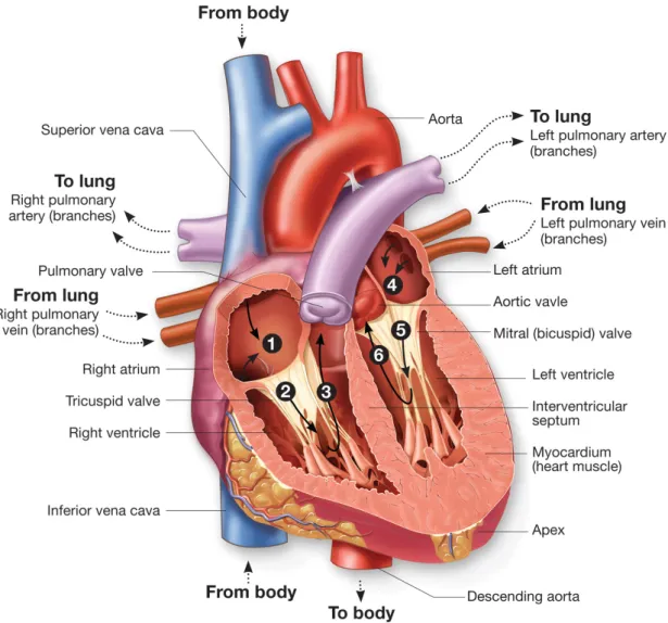
Valves are passive tissues that open and close under blood pressure forces. Anatomically, they are divided into two types, the semilunar (pulmonary and aortic) and the atrio– ventricular (mitral or bicuspid and tricuspid) valves. The semilunar valves are circular and composed of three similarly sized leaflets. Leaflets are attached to the wall at the so–called basal attachment and move freely on their opposite edge. The highest points of the basal attachment meet the other leaflets to form commissures. The atrio–ventricular valves are more complex from a morphological point of view, with unsymmetrical geome-tries. The mitral valve is composed of two leaflets whereas tricuspid valve is composed of three leaflets, all with different shapes and sizes and continuous basal attachment all around the valves. To prevent the valves from turning over, leaflets are attached to the inner walls of the ventricles by wired structures called chordae tendineae. Semilu-nar valves prevent the reverse blood flow into the ventricles during diastole while the atrio–ventricular valves prevent the reverse blood flow from ventricles to the atria during systole. The loading cycle of the valves is repeated every second so that, during a lifetime period, they will open and close nearly three billion times [Sacks et al. 2009]. A heart blood flow diagram is shown on fig. 1.
In the USA in 2010, the number of deaths directly attributable to valvular heart diseases was 23 141[Roger et al. 2012]. Taking into account valvular diseases as underlying cause of the death or being otherwise mentioned on the death certificate, the mortality number increases to 47 830. From two studies on 16 501 and 11 911 participants, the prevalence of any valve diseases adjusted to the entire US population range from 1.8 to 2.5%. This
prevalence also increases with ages : 0.3–0.7% from 18 to 44 years, 0.4–0.7% from 45 to 54 years, 1.6–0.9% from 55 to 64 years, 4.4–8.5% from 65 to 74 years and 11.7–13.3% over 75 years.
Fig. 1 – Heart circulation diagram : ¶ deoxygenated blood returns from the body to fill the
right atrium of the heart creating a pressure against the tricuspid valve ;· contracting the right atrium blood pressure forces the ticuspid valve to open filling the right ventricle ; ¸ contracting the right ventricle the pressure forces the tricuspid valve to close and the pulmonary valve to open sending deoxygenated blood toward the lungs ; ¹ oxygenated blood returns from the lungs and fills the left atrium creating a pressure against the mitral valve ; º contracting the left atrium blood pressure forces the mitral valve to open filling the left ventricle ;» contracting the left ventricle the pressure forces the mitral valve to close and the aortic valve to open sending oxygenated blood toward the body (retrieved fromhttp://biology-forums.com)
Two kinds of diseases can affect heart valves : insufficiency (or regurgitation) when the valve does not close completely, allowing a blood leak backward, and stenosis, which is more dangerous, when the tissues become stiffer (due to calcification for instance) preventing the complete opening of the valve. Depending on the severity, treatment
may be with medication but often involves valve repair or replacement with an artificial valve. More than 280 000 prosthetic valves are implanted annually worldwide [Pibarot et al. 2009] and this number will drastically increase in the next decades with population growth and aging.
We subsequently focus on the Aortic Valve (AV). Among the different valves, AV presents indeed the highest mortality. Aortic valvular diseases were directly responsible of 15 576 deaths in 2010 in the USA and considered as an underlying cause of death in 31 746 cases [Roger et al. 2012]. When valvular replacement is needed, two artificial solutions are currently available : the mechanical and the biological prostheses (fig.2). They are designed to mimic the function of natural valves.
(a) Mechanical model (b) Biological model
Fig. 2 – Examples of prosthetic AVs (retrieved fromhttp://ctsurgerypatients.org)
Mechanical prostheses Three basic types of mechanical valve design exist : bileaflet, monoleaflet and caged ball (no longer implanted) valves. They are entirely manufactured from artificial materials. Modern prostheses are made of pyrolytic carbon or titanium coated with pyrolytic carbon. The sewing ring used to suture the valve to the walls is usually made of Teflon (polytetrafluoroethylene) or polyester. Mechanical prostheses have a good durability (usually much greater than 20 years). However, they suffer from major issues. They produce a unphysiological flow that requires a lifelong anticoagulation treatment. Their rigid leaflet structure can also be responsible of cavitation leading sometimes to failure. Finally, the implantation requires an open–heart surgery. A picture of the suture of a mechanical prosthesis is shown on fig. 3.
Biological prostheses Unlike mechanical prostheses, bioprostheses mimic the anatomy of the native valves. They are made of treated (glutaraldehyde) porcine valvular tissues or bovine pericardium mounted on a supporting structure or stent. Biological prostheses of-fer a better biocompatibility. Due to their improved hemodynamics, the risk of thrombus formation is low and usually does not require the use of anticoagulant drugs. However, their durability is limited. They last between 10 to 15 years, sometimes less, and clinical follow–ups indicate that more than 50% of patients develop complications within 10 years
[Mohammadi et al. 2011]. Indeed, as bioprostheses lack living cells, degenerative processes induced by mechanical fatigue, enzymes, and calcium deposition slowly deteriorate the structural components and lead to progressive valve degeneration[Simionescu 2004]. The implantation often requires an open–heart surgery but percutaneous implantation also exists when the patient is considered to be at high or prohibitive operative risk. In that case, a percutaneous transfemoral approach is usually chosen. Nowadays, approximately 55% of the implanted prostheses are mechanical and 45% are biological [Bezuidenhout et al. 2013]. Autografts and allografts which are natural valves respectively obtained from the patient or a cadaver donor, represent together a small percentage due to their limited availability and specific surgical skills. In order to prevent or minimize the impact of the implantation, Pibarot et al. [2009] worked on a patient specific optimal selection method of the prosthesis.
Fig. 3 – AV replacement surgery with a mechanical prosthesis (retrieved from http:// biology-forums.com)
Context
The heart valves research and development area is of particular importance and currently, none of the mechanical or biological solutions are optimal. Thus, for several decades soft tissues biomechanical research has been focused on tissues mechanical characterization and numerical modeling for a better understanding of their physiological and patholog-ical behaviors. One of the main purpose of these studies was the design of engineered soft tissues with mechanical properties as close as possible to those of natural ones. Readers can refer for instance to Mohammadi et al. [2011] for a review on the model-ing and design of prosthetic aortic heart valves. Among others, Amoroso et al. [2012],
Rong Fan et al. [2013]andCourtney et al. [2006]worked on scaffold for tissue engineering.
Polymeric prostheses represent a promising alternative. They can have a similar geometry to natural valves since they are made of flexible polymer films. This design ensure the ability to closely reproduce natural hemodynamics and generally do not require anti-coagulant treatment. It is also expected that polymeric biomaterials can be treated to improve their biocompatibility, mainly hemocompatibility (minimum of inflammation and thrombogenicity) and biostability (resistance to oxidation and hydrolysis). However, polymeric prostheses currently suffer from insufficient material properties to be suitable for long–lasting implantation. After 40 years of development, results are still unsatisfac-tory. No polymeric valve has been clinically successful yet to be permanently implanted. They remain relegated to use in temporary ventricular assist devices for bridging heart failure to transplantation[Bezuidenhout et al. 2013]. Improving durability while keeping a good biocompatibility would allow polymeric prosthetic valves to become a clinical reality for surgical implantation and suitable for minimally invasive use (transfemoral ap-proach for instance).Bezuidenhout et al. [2013]propose a review of the different types of polymeric replacement heart valves currently available and identify the needs to provide longterm durability and biocompatibility. A vast literature exists on biocompatibility of polymeric materials. Reader can refer for instance to Ghanbari et al. [2009] and Ki-dane et al. [2009] for recent advances and emerging hopes in polymers, nanomaterials and surface modification techniques that can lead together to the emergence of novel biomaterials for prosthetic heart valves with improved biocompatibility and biostability. In addition, progresses in manufacturing techniques can be expected and could lead to acceptable material durability.
Objectives and outlines of the document
The design of polymeric valves may be split into a structural design and material prob-lem. This work is part of a Carnot M.I.N.E.S (Méthodes InNovantes pour l’Entreprise et la Société) project which aims to develop polymeric biomaterials for prosthetic heart
valves following a biomimetic approach. Biomimetism is a promising approach in the field of tissue engineering in order to obtain better mechanical properties from complex polymeric materials inspired from real valvular tissues. Engineered polymer materials should tend toward natural tissues mechanical properties. Thus, the objectives of this PhD thesis were essentially focused on the material problem, namely the mechanical characterization of reference natural tissues and their finite element modeling at the tissue level using relevant material models, since the development of new implants can greatly benefit from finite element modeling coupled with relevant experimental results. Due to the difficulty to obtain healthy human AV, we worked on porcine tissues.
This document consists of four chapters. Chapter 1 is dedicated to the mechanical characterization of porcine valvular tissues through biaxial tensile tests. For the purpose of this study, a custom biaxial tensile device has been designed and built at Cemef MINES ParisTech (Centre de Mise en Forme des Matériaux). The device is coupled with a digital image correlation system. Mechanical tests are performed on both frozen and fresh samples. The microstructure which is responsible for the mechanical behavior of the tissues is also studied using confocal microscopy. Chapter 2 is devoted to the numerical modeling and the implementation of three material models of the literature in a custom laboratory version of the finite element software FORGE® NXT1. A phenomenological approach is chosen in order to represent the tissue at the macroscopic level. However, selected models are able to take into account some structural information through angular integration or generalized structure tensor approaches. Hence, an algorithm is developed in order to transpose experimentally observed microstructural information into finite element models. From numerical models of chapter2and experimental results of chapter 1, a material model parameters identification is carried out in chapter 3. An inverse analysis approach using a metamodel–assited evolutionary algorithm developed at Cemef MINES ParisTech is chosen. This allows to select the most accurate model for predicting the mechanical behavior of the tissues with its associated set of material parameters. Finally, in chapter 4, firsts elements of a fluid–structure interaction model in FORGE® are introduced. The fluid part is intended to model bloodstream and interactions between blood and valvular tissues. A smoothed particle hydrodynamic method is chosen for its relative simplicity and its Lagrangian formulation. The implemented fluid solver is then weakly coupled with the finite element solver used for the solid material. The last part of the document summarizes the main developments and achievements of the current work. Suggestions of improvement and future work are also presented.
C h a p t e r
1
Aortic valve tissues
Contents
1.1 Introduction . . . . 8 1.2 Mechanical characterization . . . . 11
1.2.1 Specimen preparation . . . 11 1.2.2 Biaxial device . . . 11 1.2.3 Digital image correlation method . . . 13 1.2.4 Experimental protocol . . . 13
1.3 Fibers orientation measurement . . . 15
1.3.1 Specimen preparation . . . 15 1.3.2 Confocal laser scanning microscopy and experimental setup . . 16 1.3.3 Experimental protocol . . . 17
1.4 Experimental results . . . 18
1.4.1 Biaxial tensile tests results and discussion . . . 18 1.4.2 Confocal laser scanning microscopy results and discussion . . . 29
1.5 Summary of Chapter 1 . . . 34 1.6 Résumé en français . . . 35
1.1
Introduction
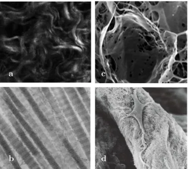
Soft tissues consist of protein fiber networks and cells immersed into a ground substance. They can grow and remodel reacting to their environment (i.e. chemical and mechanical changes). Protein fibers refer to collagen and elastin while the ground substance includes all the other components of the extracellular matrix, mainly water and glycosaminoglycans (GAGs). Collagen is the main structural protein, responsible for the tissue stiffness and cohesion. It consists of multiple tropocollagen molecules that form collagen fibrils via crosslinks. Multiple fibrils form fibers, which create a network. Several types of collagen can be defined depending on the arrangement of the protein molecules. Elastin is a highly elastic protein that contributes to the tissue cohesion and confer its elasticity. These elastic properties result from the ability of proteins to unfold reversibly allowing the tissue to go back to its original shape after stretching or contracting. Elastin is synthesized and secreted in the extracellular matrix during the growth period. With aging, the amount of available elastin decreases and is gradually replaced by collagen, making the tissue stiffer. Glycosaminoglycans consist of long unbranched polysaccharides, usually attached to a protein to form proteoglycans (PGs). Highly hydrated, they may facilitate the diffusion of nutrients and oxygen across tissues. Microscopy images of some constituents that can be found in soft tissues are shown on fig. 1.1.
a
b
c
d
Fig. 1.1 – Microscopy images of some constituents : (a) confocal image of wavy collagen fiber
bundles ; scanning electron microscopy images of (b) individual type I collagen fibers (c) elastin structure isolated from AVs using NaOH digestion[Vesely 1997](d) AV interstitial cell on collagen fiber showing long cellular extensions [Taylor et al. 2003]
AV leaflets are tri–layered structures mostly composed of wavy type I collagen, elastin and GAGs [Sacks et al. 2009]. They contain about 50% of collagen and 13% elastin on
a dry weight basis. Stella and Sacks worked on the characterization of the mechanical properties of the layers[Stella and Sacks 2007]and Buchanan and Sacks on the interlayer micromechanics[Buchanan et al. 2013]. From these studies, the fibrosa which constitutes the upper part of the leaflet, appears to be the main layer regarding the mechanical behavior. The fibrosa is the thickest layer (∼ 40% of the total thickness) and is essentially composed of undulated and strongly oriented collagen fibers. This layer is composed of 50% collagen (from which 90% of type I collagen) and 10% elastin on a dry weight basis [Mohammadi et al. 2011]. The fibrosa is considered to be the primary structural layer due to its amount of collagen organized into large fibers. The bottom layer (∼ 30% of the total thickness) is called ventricularis. Mainly composed of elastin (20%) and collagen fibers (almost 50%) this layer is highly elastic and appears to assist in reducing large radial strains [T. C. Lee et al. 2001; Vesely 1997]. Because of its high elastin concentration, the ventricularis carries slight compressive preload on the fibrosa layer at rest [Vesely 1997]. The central spongiosa layer contains a high concentration of GAGs. Its physiological function is believed to be a damping of the leaflet structure and to lubricate the fibrosa and ventricularis as they shear and deform [Eckert et al. 2013;
Lovekamp et al. 2006]. The presence of collagen and elastin fibers confer to the spongiosa a good resistance to delamination through collagen fiber interconnections between the fibrosa and the ventricularis layers. Some authors distinguish a fourth layer, the lamina arterialis, closely related to the fibrosa and located on the outflow side of the leaflet (fig. 1.2). A population of interstitial cells with characteristics of myofibroblasts also resides in AV tissues[Mulholland et al. 1997]. Their role is to maintain tissue structural integrity through protein synthesis and enzymatic degradation. Being attached to the surrounding matrix, they transmit load at the cellular level but does not contribute significantly to the leaflet mechanical behavior [Merryman et al. 2006].
1 2 3 4 1 – leaflet 2 – muscle 3 – sinus wall 4 – aortic trunk arterialis fibrosa spongiosa ventricularis
During a cardiac cycle AV cusps are submitted to three physiological loading modes : tension, shear and flexure. However, for feasibility issues, most of the characterization work that can be found in the literature are carried out on tension testing. Biaxial ten-sile tests are usually performed for valve leaflets because uniaxial loadings are known to lead to non–physiologic deformation due to fibers rotations allowed by the uncon-strained specimen edges. Also, the small strain domain of uniaxial tensile tests may lead to non–unique solutions during inverse analysis procedure. In order to estimate relevant material parameters numerous experiments over a wide range of mechanical solicitations are commonly made [Sacks 1999].Billiar et al. [2000b] have studied the multi–protocol biaxial mechanical behavior of AV fresh and glutaraldehyde–treated cusps (chemical treatment of biological tissues widely used for bioprosthetic heart valves). The leaflets time–dependent mechanical properties were investigated byStella, Liao, et al. [2007]and
Borghi et al. [2013]. AV tissues appears to be quasi–elastic materials under physiological planar biaxial loading states, with negligible time-dependent effects, unlike most of soft tissues that exhibit vicoelastic behavior. The authors speculate that this specific behavior results from the interactions between the collagen fibers and the surrounding matrix at the molecular level, especially the stabilizing effect of glycosaminoglycans. However, as the study of soft biological materials presents many theoretical and practical difficulties especially due to their highly heterogeneous structure, optical techniques are occasionally used to measure two– or three–dimensional angular fiber distributions. For instance, Billiar and Sacks developed a method using Small Angle Light Scattering (SALS) on a tensile device to quantify the fiber kinematics of tissues under biaxial stretching [Billiar et al. 1997;Billiar et al. 2000b].
As biological soft tissues usually present significant regional heterogeneity due to their local fibers arrangement, local composition and their geometrical non–uniformity, they remain challenging to be accurately characterized. Thus, the use of non–invasive video analysis systems for local full–field surface measurements, widely used in engineering re-search, seems to have a great potential. However, the reported biomechanical applications of these methods are still rather limited. Among them, the most popular technique is the Digital Image Correlation (DIC). This is an optical method which uses high resolution cameras to measure surface strain fields and displacements by tracking grey level intensity values on the sample surface during the deformation.D. Zhang et al. [2004]present the fundamentals of DIC with advanced applications to biological materials. Among exam-ples of DIC use for biomechanical applications Deplano et al. [2016], for instance, used biaxial tensile tests and three–dimensional DIC (3D–DIC or stereoscopic DIC) on porcine ascending aorta. Badel et al. [2012] used 3D–DIC coupled with a material model for the mechanical identification of layer–specific properties of mouse carotid arteries. Sutton, Ke, et al. [2008] used a microscopic 3D–DIC system for strain field measurements on mouse carotid arteries. Luyckx et al. [2014]studied human tendon tissue using 3D–DIC,
and Boyce et al. [2008], bovine cornea through inflation tests.
In this chapter a mechanical characterization of porcine AV leaflet tissues was performed using biaxial tensile experiments coupled with DIC measurements. The mechanical behav-ior of soft tissues being closely related to their fibrous architecture, confocal microscopy was also used to obtain local planar angular collagen fiber distributions in the fibrosa layer. These material and structural information will allow to accurately calibrate valvu-lar tissue models through inverse analysis procedures (see chapters 2and 3). In section 1.2we introduce the biaxial device and the experimental protocol used for the mechanical characterization of the tissues. The structural characterization, with local collagen fiber orientations measurements using confocal microscopy is detailed in section 1.3. Finally, results are presented and discussed in section 1.4. A summary concludes the chapter (section1.5).
1.2
Mechanical characterization
In this section we present the mechanical characterization of AVs through biaxial tensile tests coupled with full–field surface measurements. Due to the difficulty to obtain healthy human AV samples, we have worked on porcine tissues.
1.2.1 Specimen preparation
Two frozen (stored at −20 °C) and two fresh porcine hearts (about 5 months, 80 kg) were obtained from a local provider. AV leaflets were excised using a bistoury (fig.1.3). For each specimen, one square sample of about 10 mm side length was isolated from the central (lower belly) region of the leaflet. Similarly toBilliar et al. [2000b], samples were stored into 0.9% isotonic saline (NaCl) at room temperature during the preparation of the experiment.
Fig. 1.3 – Porcine AV leaflet excised
1.2.2 Biaxial device
A custom biaxial tensile test device, funded by MAT XPER1 company, was designed and built in our laboratory for the purpose of this study (fig. 1.4). The device is equipped
with four synchronized motorized arms, allowing a maximum displacement of 25 mm each and a minimum step of 0.05 µm. Speed ranges from 0.07 µm/s to 26 mm/s. Each arm comprise a 50 N load cell with a sensitivity of 0.001 N. Following Sun et al. [2005]
who studied the effect of boundary conditions on the estimation of the planar biaxial mechanical properties of soft tissues, specimens are maintained with a rake of five hooks on each side (at initial distance of 1 mm from each other). These boundary conditions appear to provide a better stress uniformity than clamps. The minimum area between the hooks is 7 × 7 mm2. Two cameras are placed above the specimen in order to measure full– field surface strain using a high contrast speckle pattern and 3D–DIC software. It consists of 5 Mp resolution PIKE® cameras from Allied Vision Technologies1, with a maximum
acquisition frequency of 14 fps. Low distortion fifty millimeter Schneider–Kreuznach2 photographic lenses are mounted. In order to constantly and uniformly illuminate the sample’s surface, two coherent light sources are placed above. Arms are controlled in displacement with a custom LabVIEW software (National Instruments3). Each axis stops independently when imposed force threshold is reached in order to prevent tissue degradation. During the experiment, samples are immersed into a bath of 0.9% isotonic saline at room temperature. See appendix A for further information.
Fig. 1.4 – The biaxial tensile device
1http://alliedvision.com 2http://schneiderkreuznach.com 3http://ni.com
1.2.3 Digital image correlation method
As stated in the introduction, DIC is an non–invasive optical technique that uses im-age recognition to analyze and compare grey levels of pixels from digital imim-ages of the sample’s surface. The basic principle is to build a displacement field from pictures in the initial and a deformed configurations by tracking similar points in both images (fig. 1.5). In practice, its a local collection of pixel values (called “subset”) with a signature that maximizes a similarity function which is tracked. The subset displacements and deformations are tracked by checking possible matches at several locations. Each location is graded depending on a similarity score calculated using a correlation function (clas-sically a sum of squared differences of the pixel values). High resolution and low noise cameras need to be used to take pictures of the sample during deformation. In order to make the tracking procedure possible, the surface of the sample has to be randomly and highly contrasted. If the surface does not naturally allow tracking, a high contrast speckle pattern (paint, ink, powder, . . . ) is usually applied. The method has a large number of applications for two– and three–dimensional deformation measurements for a large size of scales and a large range of time scales. To have more detailed information, the reader is highly encouraged to refer to the book written bySutton, Orteu, et al. [2009].
Fig. 1.5 – Example of subset tracking during deformation
1.2.4 Experimental protocol
First of all, the 3D–DIC system was set up. The focus of each camera was made using the maximum aperture size. Then the opening of the aperture was reduced in order to increase the depth of field during image recording. The depth of field is important to maintain focus in case of out–of–plane displacements. The system was calibrated using a standard calibration grid (a panel with a regular points grid) provided with the DIC system. The accuracy of the whole procedure is highly dependent of the qual-ity of the calibration which ensures the dimensional coherence of the system. During this process the distance from the system to the sample and the orientation of the cameras are determined. We used the VIC–3D™ software from Correlated Solutions1 for the image acquisition and the DIC processing over a selected finite area of observation.
In order to capture local strain using full–field surface measurement, a speckle pattern was made on the samples surfaces. We experienced many difficulties to find a paint
or ink able to adhere to the tissue ones immersed into the isotonic saline. In order to preserve there mechanical properties, AV tissues, which contain a lot of water, have to remain moist during the application time of the paint. However, the moisture of the leaflet surface prevents a fast drying of the paint.
After several attempts, we selected the black “Bombay India ink”, suggested inGenovese et al. [2011], which is a waterproof and quick–drying ink. Moreover, following the same authors, this ink appears to not affect the tissue mechanical behavior. To facilitate the application of the ink, the surface of the sample was quickly dried with a jet of compressed air at room temperature. Then, the ink was sprayed over the sample using an airbrush at low pressure (0.5 bar with a 0.5 mm pipe) until the speckle pattern uniformly covers the surface. The specimen dried for less than five minutes at ambient air before being mounted on the biaxial device and immersed into isotonic saline (fig. 1.6).
(a) Sample immersed (b) Speckle pattern
Fig. 1.6 – Sample mounted on the biaxial tensile devise
A small pre–load of 0.01 N was initially applied to slightly stretch the samples. From this loading state, specimens were preconditioned1 for three monotonic loadings at 0.01 mm/s with a force threshold of 0.5 N on each axis. Samples were submitted to seven loading conditions (Fx : Fy) = {(1 : 1), (1 : 0.5), (1 : 0.25), (1 : 0.1), (0.1 : 1), (0.25 : 1), (0.5 : 1)}
at 0.01 mm/s, where the couple (Fx: Fy) represents the force threshold ratio on each axis depending on the loading protocol. The maximum force threshold is fixed to 0.5 N. This value was chosen to correspond to the in vivo membrane tension peak of 60–80 N/m which occurs during diastole[Sacks et al. 2009]. This means for instance that for a (1 : 0.5) loading Fx = 0.5 N and Fy= 0.25 N. Thus, each axis stops independently when
it reaches its own force threshold. As aortic leaflet tissues showed negligible sensitivity to strain rates ranging from quasi–static to physiologic [Stella, Liao, et al. 2007], only one displacement velocity was used for the experiments. Finally, once the sample has been
1Preconditioning is usually essential in biomechanics is order to stabilize the mechanical response of
removed five thickness measurements at different locations were made using a micrometer (with a resolution of 2 µm) and averaged. Thickness measurements were made after the experiment in order to avoid damaging of the tissues and to take into account the loss of water induced by the deformation.
For the post–processing on the 3D–VIC™ software, subset size and subset overlapping (in px) were chosen with respect to the speckle pattern size, distribution and contrast (fig. 1.7) in order to obtain the best compromise between accuracy and analysis time
[Candau et al. 2016]. Note that the equivalence is of about 73 px for 1 mm. Three virtual extensometers were placed and averaged on each axis in order to measure real displacements of the sample’s boundaries. Strain was averaged in the central area of the specimen. The preconditioned state was used as reference state for strain computation.
(a) Selection of the area of interest (b) Subset grid size (29 px) Fig. 1.7 – Example of subset choice on 3D–VIC™
1.3
Fibers orientation measurement
In this section we study the collagen network structure in the fibrosa layer of porcine AVs. The objective was to get information on local fibers orientation.
1.3.1 Specimen preparation
Two fresh samples were observed using confocal laser scanning microscopy. The first sample was a square excised from the central (lower belly) region and previously tested on the biaxial tensile device. The second sample was a whole leaflet which did not undergo any ex vivo mechanical loading. The surface of the samples was carefully dried with a fabric in order to stuck them in a Petri dish, in their undeformed state, using a cyanoacrylate adhesive. The glue was applied on the ventricularis side so that the fibrosa
layer can be observed. Finally, the Petri dish was filled with 0.9% isotonic saline and fixed on the microscope stage. After a few minutes, the tissue was rehydrated and stabilized.
1.3.2 Confocal laser scanning microscopy and experimental setup
Confocal microscopy is based on the fluorescence principle, usually with a laser as light source. The laser beam goes through a pinhole, is reflected by a mirror and is finally focused on the specimen thanks to an objective lens. The surface of the specimen is scanned by moving the pinhole in an optically conjugate plane in front of a detector. Thus, only light produced by fluorescence coming from the focal plane can be detected and participates to the image formation. Out–of–focus light is optically eliminated by the confocal pinhole. Moreover, confocal microscopy allows to reconstruct three–dimensional data by recording a stack of two–dimensional images taken at successive focal planes through the sample. This is called “optical sectioning”. Readers may refer for instance to the work of Laurent et al. [1992] for further information on the working principle of confocal microscopes.
The experiments were made at the Hubert Curien laboratory (Saint–Étienne, France) on a Leica TCS SP2 SE confocal microscope (fig.1.8). The laser used was a Chameleon Vision from COHERENT®. A ×40 water immersion objective was mounted on the microscope and the zoom was set to ×1.7 to get closer to the optimal pixel size (fig. 1.9). Resulting images were 12–bit images with a total size of 220 × 220 µm2 and a pixel resolution of 1024 × 1024. In order to excite collagen fibers in all directions, a laser beam of circularly polarized light at 830 nm was used.
Fig. 1.8 – Confocal microscope Leica TCS SP2 SE form Hubert Curien Laboratory (Saint–
(a) Laser and optical system (b) Water immersion objective (×40) Fig. 1.9 – Optical system and objective
1.3.3 Experimental protocol
For both samples, the reference point was taken on a grid placed below the Petri dish aside from the sample. From this point, a series of images were made knowing the planar coordinates of each measurement and displacements were applied using a micrometric
xy travel stage. Due to the waviness of the samples’ surfaces and the spacing between
successive acquisitions, the focus had often to be made manually making the overall protocol time consuming.
On the squared sample, images acquisitions were made each millimeter in the circumfer-ential direction and half millimeter in the radial direction (fig. 1.10). An area of 5 × 5 mm2 located at the center of the sample was scanned. On the leaflet sample, images acquisitions were made with a measuring interval of 2 millimeters in both directions (fig. 1.10). An area of approximately 26 × 12 mm2 was scanned.
0.5 1
2
2
1.4
Experimental results
In this section we present experimental results obtained from biaxial tensile tests with full–field surface measurements and collagen fibers observations from confocal images of AV samples. Local fiber orientations information provided by confocal images and the mechanical response of the tissue will be later use for the identification of material models parameters using inverse analysis procedures (chapter 3). To the best of our knowledge, 3D–DIC has not previously been applied to the measurement of local biomechanical properties of AVs.
1.4.1 Biaxial tensile tests results and discussion
Conventions
Hereinafter, we define the radial and circumferential axes of tension as stated on fig. 1.11. They respectively correspond to the direction of the radius from the center of the valve and the direction following the circumference.
circumferential radial
free edge
basal attachment
commissure commissure
Fig. 1.11 – Scheme of an excised AV leaflet
Thickness measurements
The averaged thickness measurements of the samples are presented on fig.1.12. Each bar of the histogram represents the averaged thickness of the three leaflets of a valve with the maximum and minimum dispersion of leaflets’ averaged thickness from the mean. No significant dispersion between the valves samples was found, with an average value of 0.525 mm. The dispersion between the average thickness of each sample of a valve ranges from 45 to 97 µm difference with the mean value.
However, this measurements should be taken with caution due to the difficulty to obtain accurate and repeatable thickness values using a micrometer for practical reasons (softness of the tissues, heterogeneous thickness, . . . ).
Valv e1 Valv e2 Valv e3 Valv e4 0 0.2 0.4 Thic kness (mm)
Fig. 1.12 – Averaged thickness of the samples with dispersion for each valve
Tissue preservation
In order to ensure that the tissue was stabilized after preconditioning and did not yet damaged during the experiments, a (1 : 1) loading was repeated after the complete loading protocol. In fig.1.13, the first (1 : 1) loading condition of the protocol and the last one are superimposed for one sample. No significant differences in the mechanical response were found. 0 0.5 1 1.5 2 0 0.2 0.4 0.6 0.8 Displacement (mm) F orce (N) cir rad
Fig. 1.13 – (1 : 1) curves at be beginning and at the end of a complete loading protocol on a
sample
3D–DIC measurements on immersed samples
The sample being immersed, the 3D–DIC measurements can be affected by optical re-fraction at the interface between the media (i.e. isotonic saline for the sample and air for the cameras). A few people have studied this effect. In Sutton and McFadden [1999], the
authors showed that increasing errors are introduced as the angle between the optical axis and the optical interface changes. They conclude that carefully control of the rotation angle between the specimen and the viewing system during underwater experiments is sufficient to minimize the effects of orientation variations on full–field surface measure-ments. Results also indicated that slow fluid motion does not significantly affect these measurements. However, some authors have developed optimization–based or correction methods to calibrate cameras. This is the case for instance for Ke et al. [2008] who present a stereo vision and calibration methodology improving 3D–DIC measurements accuracy on submerged objects.
No correction were applied to our correlation system. However, to be sure of the mea-surements accuracy despite of the isotonic saline bath, a 3 mm displacement rigid body motion of a steel plate was captured. The strain field was measured and the displacement from DIC and the device arm were compared (fig. 1.14). No significant differences were observed between the device and the DIC measurements of the displacement. Strain fields had also negligible noise showing that results are not significantly affected by the samples immersion. 0 100 200 300 0 1 2 3 Time (s) Displacemen t (mm) Device DIC
(a) Displacements comparison (b) Nominal strain εxx
Fig. 1.14 – 3D–DIC error measurement on an immersed plate submitted to a rigid body motion
3D–DIC strain fields
Correlation parameters can significantly affect the strain field. In order to chose relevant parameters, the influence of the subset size, subset overlapping (or its opposite “step”) and filter size values was evaluated. The filter size corresponds to the number of data points used to interpolate the deformation gradient. Hence, the smoothing area is of dimension step × filter size pixels.
underestimation of the calculated strain [Candau et al. 2016]. Moreover, low step values improve the strain estimation but also significantly increase the analysis time, and too low filter size can lead to noisy strain flied. Thus, choosing a subset value adapted to the speckle pattern size and distribution, it is mandatory to select a suitable combination of step and filter size. On fig.1.15, an example of evolution of the averaged strain in a small area as a function of the smoothing area is presented for a subset size fixed to 21 px. The step ranges from 1 to 13 px and the filter size from 9 to 25. It appears that the calculated strain decreases drastically when the smoothing area increases, with a significant loss of information. A combination of step and filter size product giving the same result also give equivalent estimation of the strain. Hence we placed at the beginning of the decreasing slope with a step of 3 px and a filter size of 9 in this example. This area offers the best compromise between accuracy of the results and analysis time.
101 102
0.28 0.30 0.32 0.34
step × filter size
εxx
Fig. 1.15 – Example of nominal strain evolution function of the smoothing area for a subset size
of 21 px
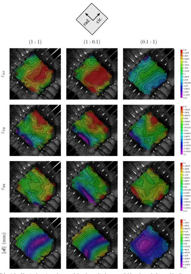
Examples of 3D–DIC strain fields ε on frozen and fresh samples are presented respectively on tab.1.1and tab.1.2. On those pictures, the strain in the radial direction corresponds to
εxxand the strain in the circumferential direction corresponds to εyy. Nominal strain was used. On both frozen and fresh samples, results showed highly heterogeneous strain fields in all directions (with also shear) for all loading conditions. Local strain concentrations generated by the boundary conditions can be observed around the rakes and at the sample’s corners. However, these local strain concentrations appear to not strongly affect the 25% central area. Indeed, the boundary conditions used do not allow large shear deformations resulting in a relatively uniform load distribution. Due to the anisotropic mechanical behavior of the tissue and the high tensile stiffness of the collagen fibers, circumferential direction deforms less than the radial direction.
rad. cir. (1 : 1) (1 : 0.1) (0.1 : 1) εxx εxy εyy k d k (mm)
Tab. 1.1 – Nominal strain and norm of the planar displacement field at the end of several loading
rad. cir. (1 : 1) (1 : 0.1) (0.1 : 1) εxx εxy εyy k d k (mm)
Tab. 1.2 – Nominal strain and norm of the planar displacement field at the end of several loading
Tension–strain data
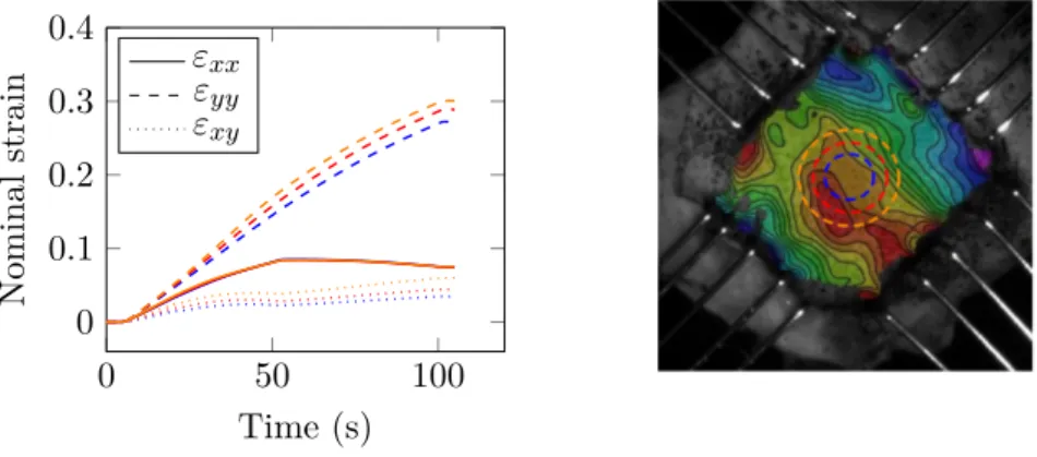
As samples are thin, a plane stress state is assumed. The classic membrane stress (or tension) in N/m was used in order to avoid the use of ambiguous thickness measurements in the stress calculations as for instance in Billiar et al. [2000b]. The strain along each direction was averaged in a circular area at sample’s center. An example of the influence of the size of this area on the strain value is shown on fig. 1.16and fig.1.17respectively for frozen and fresh tissues. In both cases, the averaged strain increases with the surface area getting closer to the boundary conditions. However, in the 25% central region the effect of the surface area on the measurements remains low. Tension–strain results for frozen and fresh samples are shown on fig. 1.18 and fig. 1.19 for a single loading. A significant dispersion of the results in both, radial and circumferential directions can be observed. Furthermore, fresh samples present meaningful differences in their mechanical response in comparison to frozen samples, such as lower strain and stress levels and a stronger coupling between the tension axes (fig. 1.20). In order to avoid the ambiguous calculation of an averaged behavior, one representative sample for each frozen and fresh tissues was chosen to present results of a full loading protocol respectively on fig. 1.21 and fig.1.22. 0 50 100 0 0.2 0.4 Time (s) Nominal strain εxx εyy εxy
Fig. 1.16 – Example of averaged strain on a frozen sample on three different areas
0 50 100 0 0.1 0.2 0.3 0.4 Time (s) Nominal strain εxx εyy εxy
0 0.1 0.2 0.3 0.4 0.5 0 50 100 150 Nominal strain T (N/m) cir rad
Fig. 1.18 – Tension–strain results for the (1 : 1) loading condition on six frozen samples for both
circumferential and radial axes
0 0.1 0.2 0.3 0.4 0.5 0 50 100 150 Nominal strain T (N/m) cir rad
Fig. 1.19 – Tension–strain results for the (1 : 1) loading condition on six fresh samples for both
circumferential and radial axes
0 0.1 0.2 0.3 0.4 0.5 0 50 100 150 Nominal strain T (N/m) cir rad
Fig. 1.20 – Example of superposition of the tension–strain results for a representative frozen
0 0.2 0.4 0 50 100 Nominal strain T (N/m) (1 : 1) cir rad 0 0.2 0.4 0 50 100 Nominal strain T (N/m) (1 : 0.5) cir rad 0 0.2 0.4 0 50 100 Nominal strain T (N/m) (1 : 0.25) cir rad 0 0.2 0.4 0 50 100 Nominal strain T (N/m) (1 : 0.1) cir rad 0 0.2 0.4 0 50 100 Nominal strain T (N/m) (0.1 : 1) cir rad 0 0.2 0.4 0 50 100 Nominal strain T (N/m) (0.25 : 1) cir rad 0 0.2 0.4 0 50 100 Nominal strain T (N/m) (0.5 : 1) cir rad
Fig. 1.21 – Tension curves on one representative frozen sample for the seven loading conditions
0 0.2 0.4 0 50 100 Nominal strain T (N/m) (1 : 1) cir rad 0 0.2 0.4 0 50 100 Nominal strain T (N/m) (1 : 0.5) cir rad 0 0.2 0.4 0 50 100 Nominal strain T (N/m) (1 : 0.25) cir rad 0 0.2 0.4 0 50 100 Nominal strain T (N/m) (1 : 0.1) cir rad 0 0.2 0.4 0 50 100 Nominal strain T (N/m) (0.1 : 1) cir rad 0 0.2 0.4 0 50 100 Nominal strain T (N/m) (0.25 : 1) cir rad 0 0.2 0.4 0 50 100 Nominal strain T (N/m) (0.5 : 1) cir rad
Fig. 1.22 – Tension curves on one representative fresh sample for the seven loading conditions
Discussion
Like most soft tissues, the AV tissue structure with a collagen fibers network embedded in an elastin matrix is responsible for their anisotropic behavior. Results presented above are consistent with literature data, highlighting the well–known highly non–linear me-chanical behavior of these tissues. This behavior is imputable to the increasing number of initially crimped collagen fibers which are activated with deformation, starting to carry a load. Liao et al. [2007] have investigated the relation between collagen fibril kinemat-ics (rotation and stretch) and tissue–level mechanical properties of mitral valves tissues under biaxial loading using SALS. According to their findings, collagen fibrils remain in their unstrained configuration until the beginning of the highly non–linear region of the tissue–level stress–strain curve. From tension–strain curves (fig.1.21and fig.1.22), it can be clearly observed that the tissue is much more compliant in the radial direction than in the circumferential one, inducing large extensibility disparities. This mechanical response has to be compared to the fibrous structure. However, from an histology point of view it is known that collagen fibers in the fibrosa are mainly oriented in the circumferential direction (fig.1.11), making the tissue very stiff. In the fibrosa, elastin plays a minor role and is only predominant in terms of mechanical response at low stretch, when most of the collagen is crimped. In the ventricularis, elastin fibers are predominately oriented in the radial direction. According to Vesely [1997], in this layer elastin participates equally with collagen during initial circumferential stretches but dominates the radial behavior, making the tissue response more compliant. This radial extensibility is important during valve closure phase, in order to prevent retrograde flow by ensuring leaflets’ co–adaptation.
For both, frozen and fresh samples 3D–DIC measurements showed highly heterogeneous strain fields (tab. 1.1 and tab. 1.2). Thus, a complete inverse procedure on the force– displacement is required to exploit the experimental results. However, the strain and stress levels were significantly lower for fresh tissues. A strong coupling between the axes can also be observed. When one axis stops moving, the displacement on the other axis is responsible for fibers rotations. These fibers rotations induce significant realignments and decreasing strains can occur on the immobile axis. Thus, decreasing strain appears in the circumferential direction for conditions with low circumferential strain and large radial strain ((0.1 : 1) for instance). This phenomenon is much more visible on fresh samples showing that the freezing of the tissue probably damages the fibrous structure. Experimental results showed an important scattering of the mechanical response between the samples, for both fresh and frozen conditions, but no significant difference between the leaflets of a same valve (or from different valves) was observed. The last observation should be taken with caution due to the limited number of specimens. For instance, in a recent study on the mechanical properties of aged human cardiac valves (70.1 ± 3.7 years old) some differences between non–coronary, left coronary and right coronary aortic leaflets’ mechanical response were highlighted[Pham et al. 2017]. A good agreement was