Recognizing Art Style Automatically in painting
with deep learning
Adrian Lecoutre adrian.lecoutre@insa-rouen.fr
LAMSADE, INSA de Rouen,76800 Saint- ´Etienne-du-Rouvray, France
Benjamin Negrevergne benjamin.negrevergne@dauphine.fr
Florian Yger florian.yger@dauphine.fr
LAMSADE, CNRS, Universit´e Paris-Dauphine, PSL Research University, 75016 Paris, France
Editors: Yung-Kyun Noh and Min-Ling Zhang
Abstract
The artistic style (or artistic movement) of a painting is a rich descriptor that captures both visual and historical information about the painting. Correctly identifying the artis-tic style of a paintings is crucial for indexing large artisartis-tic databases. In this paper, we investigate the use of deep residual neural to solve the problem of detecting the artistic style of a painting and outperform existing approaches to reach an accuracy of 62% on the Wikipaintings dataset (for 25 different style). To achieve this result, the network is first pre-trained on ImageNet, and deeply retrained for artistic style. We empirically evaluate that to achieve the best performance, one need to retrain about 20 layers. This suggests that the two tasks are as similar as expected, and explain the previous success of hand crafted features. We also demonstrate that the style detected on the Wikipaintings dataset are consistent with styles detected on an independent dataset and describe a number of experiments we conducted to validate this approach both qualitatively and quantitatively. Keywords: Art style recognition, Painting, Feature extraction, Deep learning,
1. Introduction
The Metropolitan Museum of New York has recently released over 375,000 pictures of public domain art-work that will soon be available for indexation (met,2008). However, indexing artistic pictures requires a description of the visual style of the picture, in addition to the description of the content which is typically used to index non-artistic images.
Identifying the style of a picture in a fully automatic way is a challenging problem. Indeed, although standard classification tasks such as facial recognition can rely on clearly identifiable features such as eyes or nose, classifying visual styles cannot rely on any defini-tive feature. As pointed by Tan et al. (2016) the problem is particularly difficult for non-representational art-work.
Several academic research papers have addressed the problem of style recognition with existing machine learning approaches. For exampleFlorea et al.(2016) evaluated the perfor-mance of different combinations of popular image features (Histograms of gradients, spatial envelopes, discriminative color names, etc.) with different classification algorithms (SVM, random forests, etc.). Despite the size of the dataset and the limited number of labels to predict (only 12 art movements in total), they observed that several styles remain hard to
distinguish with these techniques. They also demonstrate that adding more features does not improve the accuracy of the models any further, presumably because of the curse of dimensionality.
In 2014, Karayev et al. observed in that most systems designed for automatic style
recognition were built on hand-crafted features, and manage to recognize a larger variety of visual style using a linear classifier trained with features extracted automatically using the deep convolutional neural network (CNN). The CNN they used was AlexNet (Krizhevsky
et al.,2012) and was trained on ImageNet to recognize objects in non-artistic photographs.
This approach was able to beat the state-of-the-art, but the authors obtained even better results on the same datasets using complex hand-crafted features such as MC-bit (Bergamo
and Torresani, 2012). More recently Tan et al. (2016) addressed the problem using a
variation of the same neural network and managed to achieve the best performance with a fully automatic procedure for the first time, with an accuracy of 54.5% over 25 styles.
In this paper, we further improve upon the state of the art and achieve over 62% accuracy on the same dataset and using a similar experimental protocol. This important improvement is due to two important contributions described below.
First, we demonstrate that Residual Neural Networks which have proven to be more ef-ficient on object recognition tasks, also provide great performance on art style recognition. Although it may be expectable, this result is not immediately implied by the success of Resnet on object recognition, since art style recognition requires different types of features (as it will be shown in the paper). As a matter of fact, state-of-the-art neural network archi-tectures for object recognition have not always been state-of-the-art for art style recognition. (See,Karayev et al.(2014) discussed above.)
Second, we demonstrate that a deeper retraining procedure is required to obtain the best performance from models pre-trained on ImageNet. In particular, we describe an experiment in which we have retrained an increasing number of layers — starting from retraining the last layer only, to retraining the complete network — and show that the best performances with about 20 layers retrained (in contrast with previous work where only the last layer was retrained). This result suggests that high level features trained on image net are not optimal to infer style.
In addition, the paper contains a number of other methodological insights. For example, we show that the styles learnt using one dataset are consistent with the styles from another independent dataset. This shows that 1) our classifier does not overfit the training dataset 2) styles are consistent with the artistic style defined by art experts.
The rest of the paper is organized as follows : in Section2we formally state the problem that is being addressed in this paper and we present various baselines we used to assess the performance of our new approach, then, in Section 3 we describe our approach, and present experimental results in Section 4. Finally we conclude with some comments and future directions.
2. Related works
Creative work have attracted much attention in the AI community, maybe because of the philosophical questions that it raises or because of the potential applications. As a result, a number of publications have discussed the problem of art generation and art style
recog-nition in several artistic domains such as visual arts (Gatys et al., 2015) or music (Oord
et al.,2016;Huang and Wu,2016).
In the domain of visual art generation,Gatys et al.(2015) were able to build a model of a specific painting style and then transfer it to non-artistic photographs1. From a technical perspective, art generation is not very different from art style recognition: in both cases, the first step is to accurately model one or several artistic styles. Gatys et al.(2015) started by training a deep VGG net (Simonyan and Zisserman,2014) with a large number of pictures from a given artistic style. Then they generated an image that compromised the matching of the style with the matching of the original input image. However, one important difference with the problem of art style recognition, is that the model needs to separate style from content as much as possible in order to successfully transfer the style to a new content. In style recognition, we use the description of the content as an additional feature to recognize the style (e.g., a person is more likely to appear in an impressionist painting than in an abstract painting).
The problem of art style recognition has been directly addressed by a number of other publications. The techniques proposed usually work either with pre-computed features such as color histograms, spacial organisation and lines descriptions (Florea et al., 2016;
Liu et al., 2015), or directly with the image itself (Saleh and Elgammal,2015; Tan et al.,
2016). Liu et al.(2015) have been able to achieve good results using pre-computed features
using multi-task learning and dictionary learning. To achieve this result, they propose to discover a style-specific dictionary by jointly learning an artist-specific dictionary across several artists having painted with the same style.
Although working with pre-computed features can be useful to better understand the behaviour of the classifier, the resulting classifiers do not generally achieve the best accuracy. Learning the features automatically from the images (with convolutional neural networks) generally obtain better results as shown by the work by Tan et al. (2016) which achieved 54% top-1 accuracy on 25 classes.
3. Problem statement & methodology
In this paper, we are interested in developing a machine learning method able to recognize the artistic style of a painting directly from an image of this picture (i.e. a 2-dimensional array of RGB pixels). We evaluate the performance of various deep artificial neural networks at this task, including the state-of-the-art deep residual neural networks proposed by He
et al. (2016). In this section, we describe the datasets and the training methodology that
we have used to design a new art style classifier that we call RASTA which stands for Recognising Art STyle Automatically.
3.1. Datasets
To train our models, we use the Wikipaintings dataset, a large image dataset collected from WikiArt following the experimental protocol used byKarayev et al.(2014) and byTan et al.
(2016). To test the models, we use two datasets: one from Wikipaintings and another one from an independent source.
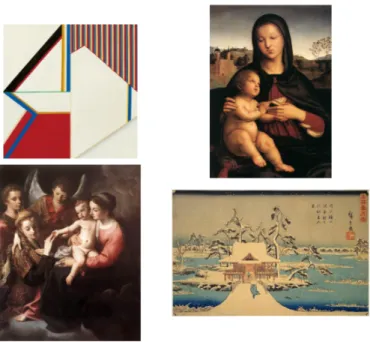
Figure 1: Four examples of images of the Wikipainting dataset. From left to right and top to bottom : a. Hereditarius No.1-68-A by Park Seo-Bo (Minimalism) - b. Madonna and Child by Raphael (High Renaissance) - c. The Mystic Marriage of St Catherine by Annibale Carracci (Baroque) - d. Benzaiten Shrine at Inokashira in Snow by Hiroshige (Ukiyo-e)
3.1.1. The Wikipaintings datasets
We have collected images on the WikiArt website2 with their respective artistic style name. The resulting dataset contains 80,000 images tagged with one corresponding style chosen among the 25 following styles: Abstract Art, Abstract Expressionism, Art Informel, Art Nou-veau (Modern), Baroque, Color Field Painting, Cubism, Early Renaissance, Expressionism, High Renaissance, Impressionism, Magic Realism, Mannerism (Late Renaissance), Mini-malism, Naive Art (Primitivism), Neoclassicism, Northern Renaissance, Pop Art, Post-Impressionism, Realism, Rococo, Romanticism, Surrealism, Symbolism and Ukiyo-e. Sam-ple images from the Wikipaintings dataset are visible in Figure 1. As we can see, some paintings can have similar content, but different style (e.g. painting (b) from High Renais-sance and painting (c) from Baroque).
The first 66,549 images of this collection are used to form the wikipaintings-train dataset (i.e. about 80% of the full dataset). The next 7,383 images (about 10% of the train dataset) are used to form the wikipaintings-validation dataset and the final 8,222 images (10% of the full dataset) are used to form the wikipaintings-test dataset. The class distribution is kept the same in all three datasets, and the full dataset distribution is visible in Figure2.
0 2000 4000 6000 8000 10000 12000 Number of images per class
Early_RenaissanceUkiyo-e
Art_Nouveau_(Modern)Northern_Renaissance
Mannerism_(Late_Renaissance)Post-ImpressionismAbstract_Art
Cubism Minimalism Impressionism
High_RenaissanceExpressionismPop_Art
Abstract_ExpressionismNaïve_Art_(Primitivism)Symbolism
Magic_RealismArt_InformelRococo
RomanticismBaroqueRealism
NeoclassicismSurrealism Color_Field_Painting 1330 1178 4163 2405 1192 5998 1006 1686 1267 12164 1275 5844 1129 2091 2026 4063 1011 969 1928 6569 3992 10090 2700 4799 1258
Figure 2: Class distribution of the Wikipainting dataset.
3.1.2. The ErgSap and ErgSap-minus-wikipaintings testing datasets
Styles may be very coherent within the Wikipainting datasets, but may not correspond to any style recognizable by experts outside the WikiArt community. In order to evaluate the generality of the styles identified by the models trained with the Wikipaintings datasets, we need extra datasets collected from an independent source.
To achieve this, we use a dataset provided by the author of ErgSap3, a visual art gallery application. The dataset contains almost 60,000 images of paintings which are available in the public domain.
Not all the classes from the Wikipainting dataset are represented in the data provided by ErgSap, and some classes have different names. In order to make the datasets compatible we remove classes from ErgSap that are not represented in Wikipaintings. We end up with a dataset of 14 classes : Neoclassicism, Romanticism, Impressionism, Baroque, Mannerism (Late Renaissance), Realism, Rococo, Post impressionism, Expressionism, Symbolism, Cu-bism, Art Nouveau, Symbolism, Ukiyo-e, Naive Art. The resulting ErgSap dataset contains 40,437 images distributed in the 14 classes as shown in Figure3 (a).
There is no guarantee that the paintings in the ErgSap dataset are absent from the wikipaintings-train dataset as a training example. In fact, this is likely to happen since many images are pictures of famous paintings. We estimate the overlap between the two datasets by simply comparing meta data and removing the images with meta data similarities (author name, picture name and year).
Using this procedure, we estimated an overlap between Wikipaintings and ErgSap to 53%. To accurately estimate the accuracy on a fully independent dataset, we build a new dataset with only the images from ErgSap that do not appear in the Wikipaintings dataset. We call this new dataset ErgSap-minus-wikipaitings. The dataset contains 19,077 images distributed in the 14 classes as shown in Figure3 (b).
0 2000 4000 6000 8000 Number of images per class
Ukiyo-e Art_Nouveau_(Modern) Mannerism_(Late_Renaissance)Cubism Impressionism Post_impressionismExpressionism Naïve_Art_(Primitivism)Symbolism Rococo RomanticismBaroque Realism Neoclassicism 39 471 430 88 4135 2987 506 209 1057 975 2667 2235 2531 747 95 1667 899 224 8952 4447 1128 312 2218 1778 6197 4509 6782 1229 (a) Ergsap (b) ErgSap-minus-wikipaintings
Figure 3: Class distribution of Ergsap dataset and Ergsap-minus-wikipaintings dataset.
3.2. Neural networks architecture
We used two types of networks, first a network based on AlexNet architecture which was used in (Karayev et al.,2014), then we used the state-of-the-art residual neural network as described in (He et al.,2016) (ResNet). Residual neural networks provide very interesting results on object detection tasks, and pre-trained weights are available (on Keras frame-work). It is now the state-of-the-art network for many image related tasks and in some applications, it has been shown that using a ResNet instead of a more classical network boosted the performances of the method (Cazenave,2017).
3.2.1. AlexNet
The input of the AlexNet network is a 227 × 227 × 3 matrix. Its structure is made of five convolutional layers and three fully connected layers. Convolutional layers have respectively filter of size 11 × 11, 5 × 5, 3 × 3, and 3 × 3. They each respectively generate 96, 256, 384, 384, and 256 feature maps. Three max-pooling layers follow the first, third and fifth convolutional layer. Then there are 4096 neurons in the 2 following fully connected layers. Dropout is implemented after each of those two fully-connected layers.
3.2.2. ResNet
The ResNet has input dimensions of 224 × 224 × 3. Its architecture is composed of different blocks, where each block uses a ”shortcut connection”. This shortcut connection can be a simple identity connection (id-block), or a connection with a convolutional layer (conv-block). The shortcut-ed part of the block uses 3 convolutions, with various number of filters for each block. The first and third convolution of this group use filters sizes of 1 x 1, and the second one is usually 3 x 3. At the end of a block, the features of the shorcut part and the shortcut-ed part are added. Each convolutional layer is followed by a batch-normalization layer.
We mainly used a ResNet50 architecture in our experiments. The ResNet50 starts with a convolutional layer with a filter size of 7x7, generating 64 filters, followed by a batch-normalization layer, an activation layer and a max-pooling layer. Then there are 4 groups
of blocks, each starting with a conv-block. Each group contains respectively 1, 3, 5 and 2 id-blocks. The ResNet50 contains in total 53 convolutional layers, hence its name.
We also used a ResNet34 architecture in our experiments, which is very similar to the ResNet50, except that the shortcut-ed part of the blocks uses 2 convolutional layers instead of 3, which reduces the total number of convolutional layers to 34.
In both types of architectures (ResNet and AlexNet), rectified Linear Unit (ReLU) is used as the activation function for all weight layers, except for the last layer that uses softmax regression. A fully-connected layer ends each network, of which the number of neurons corresponds to the number of classes.
3.3. Training procedure
Goodfellow et al. (2016) estimate that to achieve human-level classification performance,
a neural network needs to be trained with about 5,000 labels per class. Despite being a relatively large dataset compared to other dataset in art style recognition, the wikipaintings-train dataset only has about 2,662 images per class on average.
To overcome this limitation,Tan et al.(2016) used models pre-trained for object recogni-tion on ImageNet. In order to predict style instead of content occurrences, the last softmax layer is retrained for style recognition using the Wikipaintings dataset. In their experiments,
Tan et al.(2016) show that this technique performs better than a model fully trained from
scratch using only the Wikipaintings dataset.
This result demonstrates that features generated to recognize objects can also be used to recognize style. Following the results in (Yosinski et al., 2014), we conjecture that this not always true.
To validate this hypothesis, we retrain a variable number of layers ranging from one layer only (as in (Yosinski et al.,2014)) to the complete network. We start from the last layer, to the very bottom one. As we will show in the experimental section the best performance is obtained when we retrain approximately 20% of the layers. This provides evidence that building new features that are specific to the task was indeed necessary.
3.4. Additional training and testing improvements 3.4.1. Bagging
In order to increase accuracy and stability of our classifier we introduced the bagging tech-nique as described by Cazenave (2017) for the game of Go. It consists in averaging the output of different predictions produced by the model on several variations of input data. As shown by Cazenave, bagging can increase overall accuracy without degrading the effi-ciency of the classifier too much. In case of art style recognition, we generate two variations of the input data (the picture) by flipping the picture horizontally, (intuitively, the style of a picture should be invariant to horizontal flip) and average the results.
3.4.2. Dataset augmentation
Image augmentation often used to limit the cost of tagging images manually. It consists in using images that are already in the training dataset and manipulating them to create
many altered versions of the same image (Wong et al., 2016). In contrast with bagging, dataset augmentation but operates during the training phase.
In order to increase the robustness of our models and their ability to generalise to a broad range of unknown pictures, we augmented the training dataset by applying distortions to the input images. We used the following distortions: random, horizontal flips, rotations, axial translations and zooming.
Horizontal image flip happens with a user defined probability which we empirically set to 0.5. For rotations, axial translations and zooming, a random variable is drawn uniformly each time an image is selected as a training example, and controls the extent of the distortion. For horizontal and vertical transitions, a variable is drawn between 0 and the image width or the image height respectively and controls the number of pixel shifted. For rotations the variable is drawn between 0 and 90◦. For zooming, a variable is drawn between a factor 0 (no zoom) and 2 (2× zoom).
4. Experiments and results
In this experimental section, we aim at answering the following scientific questions. Q1: How do residual neural network architectures which are state-of-the-art in object recognition compare to the AlexNet architectures (used in (Tan et al., 2016)) when they are used to recognize image style? This question is discussed in Section 4.2. Q2: What proportion of the network should be retrained to obtain the best performance? This question is discussed in Section 4.3. Q3: What is the impact of the optimizations described in Section 3.4 and how does it perform in our test datasets? This question is addressed in Section 4.4. After addressing these questions with quantitative experiments and results, we also provide a qualitative analysis of the results in Section4.5
4.1. Experimental protocol
In this experimental section, we conduct our experiments on the datasets described in Section 3. The train set is used for training the models, the wikipaintings-validation set is used for wikipaintings-validation operations such as early stopping and parameter tuning, and the test sets are used to measure final accuracy. In some of our experiments, we used models pre-trained on ImageNet. To pre-train a model, we simply load the model parameters (i.e. the weights) computed by their original authors instead of reproducing the full training procedure on ImageNet. This saves computation time and also guarantees that the models are state-of-the-art. The weights of the models were downloaded for AlexNet4 and found in the Keras framework for the ResNet with 50 convolutional layers (ResNet50)5. The implementation was written in Python, using the Keras framework with Tensorflow as a backend. The experiments were run on Nvidia GTX 1080Ti GPUs. All datasets and weights as well as a fully functional web application are available online6 .
4. http://files.heuritech.com/weights/alexnet_weights.h5
5. Seehttps://keras.io/applications
6.http://www.lamsade.dauphine.fr/~bnegrevergne/webpage/software/rasta/rasta-web/src/
0 10 20 30 40 50 Number of epochs 0.15 0.20 0.25 0.30 0.35 0.40 0.45 0.50 Va lid ati on ac cu rac y Pretrained AlexNet Pretrained ResNet Re-trained ResNet ResNet 34
Figure 4: Baseline comparison (validation set)
0 10 20 30 40 50 Number of epochs 0.2 0.3 0.4 0.5 0.6 0.7 0.8 0.9 Tr ai ni ng a cc ur ac y Pretrained AlexNet Pretrained ResNet Re-trained ResNet ResNet 34
Figure 5: Baseline comparison (train set)
4.2. Performance of residual neural network at image style recognition
In this experiment, we assess the performance of various convolutional neural network for the problem of recognizing artistic style. We compare the AlexNet network which was used by Karayev et al. (2014) and by Tan et al. (2016) with the two Residual Neural Network configurations with 34 and 50 convolutional layers. For AlexNet and ResNet50, we compare the performance of models pre-trained on ImageNet with models trained from scratch with the wikipaintings training set. Note that we did not evaluate the performance of ResNet34 pre-trained on ImageNet as no pre-trained model was available in Keras. In this first experiment, only the last layer of the residual neural network is retrained following the procedure described byTan et al.(2016).
The results of these experiments are presented in Figure 4 and 5, and the final Top-1, Top-3 and Top-5 accuracy for the best models are provided in Table1.
The first thing we can observe in Figure 4 is that pre-trained models achieve better accuracy on validation set, and with a fewer number of training epochs. This result agrees with the results fromTan et al.(2016) on AlexNet, but also applies to the ResNet
configu-Architecture Top-1 Top-3 Top-5 Pre-trained AlexNet accuracy (6th layer features) 0.378 0.627 0.733 Pre-trained ResNet50 accuracy 0.494 0.771 0.874
Table 1: Top-k accuracies for retrained models
rations. Furthermore, after 25 epochs, we can see that several models trained from scratch begin to overfit to the training set. This is particularly visible for ResNet50 which reaches over 90% accuracy on the training set, but does not perform any better on the validation set. This is likely due to the limited number of training examples (60,000 images) and the large number of parameters in ResNet50.
ResNet34 does not overfit like ResNet50, probably because of the smallest number of parameters. However, its validation accuracy is very unstable, and the train accuracy shows a very slow convergence.
If we now focus on the models which have been pre-trained with ImageNet, ResNet50 outperforms AlexNet by 10% over the 25 classes. This is also true when we look at the Top-3 and Top-5 accuracy available in Table 1
4.3. Impact of retraining
In the previous experiments, we have compared models pre-trained on ImageNet and with the last layer retrained for the task of art style recognition. This approach is standard and works well when the initial classification task is closely related to the target classification task. (i.e. that the same high level features can be used for both tasks).
In Section 3.3, we conjectured that a deeper retraining could contribute to improve the accuracy by generating features specific to style recognition. To validate this hypothesis, we compare the performance of the best architecture (ResNet50) with a variable number of layers retrained ranging from 1 (the top-layer) layer only to a full retrain. As mentioned
in (Yosinski et al.,2014), a full-retraining is not necessarily the best approach since deeper
layers in image recognition tasks are very similar among different tasks. They generally describe very low-features, common to a lot of image classification tasks. Moreover,Yosinski
et al.(2014) conjecture that keeping the learned weights as initializer for the trained layers
can often be more efficient than retraining from a random initialization.
We retrained the pre-trained ResNet50 architecture with variable number of trainable layers, and initialized randomly the weights or kept the Imagenet weights. The rest of the layers are frozen with ImageNet weights. The results of these experiments are presented in Figure 6.
We can first notice that in both cases, the peak accuracy is achieved with almost 20 top-layers retrained out of 106 (i.e. approximately ∼ 20% of the network retrained). With less trainable layers, we can see that initializing weights randomly can give slightly better results. Around and after the peak, an ImageNet initialization outperforms the random initialization. We can suppose that ImageNet information contained in the top layers is not really transferable to our classification task. It corresponds to high-level features, that are more specific to content recognition than style classification. It could even cause the gradient descent to be stuck in a local minima. For deeper layers, since they generally describe low-level features (with filters usually resembling to Gabor filters or color blobs),
0 20 40 60 80 100 Number of layers retrained
0.30 0.35 0.40 0.45 0.50 0.55 0.60 0.65 0.70 Va lid ati on ac cu rac y
Initialization with imagenet weights Random initialization
Figure 6: Validation accuracy with respect to the number of retrained layers Evaluation type Top-1 Top-3 Top-5
Without bagging 0.601 0.858 0.933 With bagging 0.611 0.863 0.936 Table 2: Impact of bagging on the accuracy
an ImageNet initialization can be very useful, and induces some speed in training, and a gain in accuracy. It confirms the assumption that deeper layer neurons are not specialized to only one specific task. Moreover, training too many layers (regarding the size of our train set) can lead the model to overfit, which explains the accuracy drop in both curves after 20 trainable layers.
4.4. Improving accuracy 4.4.1. Bagging
As we can see in Table 2, bagging makes our model gain almost 1% on Top-1 accuracy. This result supports the assumption that characteristics determining painting styles do not generally rely on the horizontal orientation. It is coherent with the gain observed when applying bagging to other applications where symmetries occur, as in Go (Cazenave,2017). 4.4.2. Distortion
Encouraged by the positive results on bagging, we tried to augment our dataset by gener-ating artificial data. However, the results reported in Table3show a mild improvement on Top-1 results and a deterioration according to Top-3 and Top-5 metrics. Behind the data augmentation, there is an assumption that a particular image will remain of the same class if we apply a distortion to it. This is true for most image recognition tasks : for example, if the task is to recognize animals, a cat should be detected in an image even if it is upside-down. However, this is not true for all style of paintings. We remark that the images in our dataset are perfectly centered without any background or foreground around the painting. Hence, with such a clean dataset, the data augmentation may not be necessary. If we let
Distortion rate x Top-1 Top-3 Top-5 0 0.611 0.863 0.936 0.1 0.625 0.813 0.934 0.2 0.621 0.862 0.934 0.3 0.624 0.860 0.932 0.4 0.623 0.859 0.933 Table 3: Distortions effects on accuracy Dataset Top-1 Top-3 Top-5 Wikipaintings-test 0.628 0.860 0.933 Ergsap 0.630 0.859 0.931 Ergsap-minus-wikipaintings 0.629 0.852 0.925 Table 4: Test accuracy on different test sets
users upload their own picture of paintings, data augmentation may become necessary to cope with the data variability.
4.4.3. Results on test set and new dataset
Up to this point, the model selection and the different optimizing parameters (number of layers, distortion rate) have been selected regarding the results on the wikipaintings-validation set. To avoid any data leakage and ensure unbiased results, we have to evaluate our final model with an unseen dataset. Moreover, since the wikipaintings-test dataset comes from the same source, we evaluate the performance of our model on an external dataset (Ergsap and Ergsap-minus-wikipaintings). Results are presented in Table4. As we can see, we obtain very similar results on Ergsap, Ergsap-minus-wikipaintings and wikipaintings-test, so our model is not specific to Wikipaintings or the validation set.
4.5. Qualitative analysis 4.5.1. Per class analysis
As shown in Table 5, styles like Ukiyo-e, Minimalism or Color Field Painting have very distinct visual appearance and show in general the best results. To be as fair as possible, we provide results of Recall and Precision as the class repartition on the test set is un-balanced. As a remark, the classes having the worst performances (e.g. High Renaissance and Mannerism or Abstract art and Art informel) correlate to classes that are visually and historically close and for which few data are available (see Figure2).
Some noticeable values can be extracted from the confusion matrix in Figure 7. We identified some of the most important mis-classifications on our test set. For the most, the two mixed styles share some common conceptual ground. For example, 18% of images coming from Post-Impressionism are classified as its elder brother, Impressionism. 22% of Mannerism images are classified as Baroque, knowing that the Mannerism style is sometimes considered as an early stage of Baroque. 17% of High Renaissance images are classified as Northern Renaissance, which are 2 styles that come from the same root. 21% of Art Informel images are classified as Abstract Expressionism, and the Art Informel is often considered as the European equivalent of American Abstract expressionism.
Table 5: Accuracy, recall and precision per class (sorted by accuracy) Style Accuracy Recall Precision
Ukiyo-e 99.695 88.034 90.4
Minimalism 99.146 76.984 70.3 Color Field Painting 99.110 72.800 70.0 Early Renaissance 99.061 66.165 73.3 Magic Realism 98.927 53.465 56.8 High Renaissance 98.915 43.307 76.4 Art Informel 98.793 33.333 47.8
Pop Art 98.781 56.250 55.3
Mannerism (Late Renaissance) 98.671 42.857 55.4 Abstract Art 98.427 47.000 38.2 Naive Art (Primitivism) 98.220 59.406 65.2
Rococo 98.208 65.104 61.0 Northern Renaissance 98.098 83.750 63.2 Cubism 97.976 61.905 50.5 Neoclassicism 97.964 62.593 71.9 Abstract Expressionism 97.891 51.196 60.1 Baroque 96.878 68.170 67.8
Art Nouveau (Modern) 96.196 62.500 62.5 Symbolism 96.000 49.015 62.2 Surrealism 93.989 68.894 49.0 Post-Impressionism 93.806 43.907 60.5 Romanticism 93.513 62.652 58.9 Expressionism 93.281 51.370 52.9 Impressionism 91.623 70.970 72.1 Realism 89.745 62.934 57.6
This way, we can perceive a glimpse of the relation between artistic styles. Our model seems to generally struggle on differentiating historically close styles, as a human would probably do.
4.5.2. t-SNE
Another way to evaluate the encoding quality of our model is to represent visually the dataset on a 2D space, using a t-SNE algorithm. As described in (Maaten and Hinton,2008), t-SNE maintains the global geometry of the data and allows us to picture the repartitions of our points following their corresponding class. In few words, t-SNE finds the coordinates of n points in a 2-dimensional space so that the distances between those points behave similarly as the distances between the original points. It formulates as the minimization of a KL divergence involving the distance matrices of both input and output data.
For each data point, we extracted the 2,048 features from the penultimate layer (be-fore the last fully connected layer), and first reduced the dimensionality to 50 features by applying a PCA reduction. Indeed, t-SNE can lose efficiency when applied on very high-dimensional data. Afterwards, a 2-high-dimensional representation of the dataset is found by computing the t-SNE.
Applying a dimensionality reduction using a t-SNE reduction on all the data and over 25 classes can lead to a hardly readable Figure, so we only took some subsets of 3 classes coming from the wikipainting-test dataset. We selected the 3 classes giving the best recall
Im pre ssi on ism Mi nim ali sm Re ali sm Ba roq ue Ma nn eri sm _(L ate _R en aissa nc e) Ar t_No uv ea u_( Mo de rn) Sy mb oli sm Cu bism Ro ma nti cism Ne oc lassi cism Ab str ac t_E xp ressi on ism Ea rly _R en aissa nc e Co lor _F iel d_Pa int ing Ar t_I nfo rm el Ex pre ssi on ism Ro co co Ma gic _R ea lism Uk iyo -e Po st-Im pre ssi on ism No rth ern _R en aissa nc e Su rre ali sm Hig h_R en aissa nc e Na ïve _A rt_ (Pr im itiv ism ) Ab str ac t_A rt Po p_A rt ImpressionismMinimalism Realism Baroque Mannerism_(Late_Renaissance)Art_Nouveau_(Modern) SymbolismCubism Romanticism Neoclassicism Abstract_ExpressionismEarly_Renaissance Color_Field_PaintingArt_Informel ExpressionismRococo Magic_RealismUkiyo-e Post-Impressionism Northern_RenaissanceSurrealism High_Renaissance Naïve_Art_(Primitivism)Abstract_Art Pop_Art 0.0 0.1 0.2 0.3 0.4 0.5 0.6 0.7 0.8
Figure 7: Confusion matrix
Figure 8: 2D visualisaion of the dataset. From left to right : (a) Ukiyo-e, Color Field Painting and Northern Renaissance (b)Ukiyo-e, Baroque and Mannerism
results(Ukiyo-e, Northern Renaissance and Color Field Painting) (a). We also selected the 2 class generating the most misclassifications (Mannerism with Baroque) and the class with the best recall (Ukiyo-e) (b).
As we can see on Figure 8, the second t-SNE illustrates a great overlap between Man-nerism and Baroque. The Ukiyo-e is better separated from the two others classes, but it still has some mixed points. Such a visual analysis correlates with the results in Table5.
5. Conclusion
In this paper, we successfully applied a deep learning approach to achieve over 62% accuracy on WikiArt data. This improvement is mainly due the use of a residual neural network and to the importance of retraining. However, the obtained results, we provided some empirical evidences for our choices of parameter and then brought a methodological contribution.
As suggested by our experiments, the use of bigger datasets should enable to learn more layers of our deep networks and should improve the accuracy of our models. Hence, we plan to extend our datasets so that we can perform a full retraining of our deep models.
As a future work, we plan to apply the deep network analysis proposed in (Montavon
et al., 2016; Binder et al., 2016), once it will be available for ResNet, in order to have an
understanding of the learnt feature. By analyzing every layer in this way, we will be able to see how the networks characterize a given style.
Acknowledgments
We would like to acknowledge the support of grid5000 for our experiments and to thank Tristan Cazenave, Florian Sikora and Chesner D´esir for their feedback and helpful com-ments. We would also like to thank the team of Google Arts and Culture for the interesting discussions. Finally, we would like to thank Lars Wagner for starting the discussion on artistic style and machine learning.
References
The Met Makes Its Images of Public-Domain Artworks Freely Available through New Open Access Policy.http://www.metmuseum.org/press/news/2017/open-access, 2008. [On-line; accessed 14-February-2017].
Alessandro Bergamo and Lorenzo Torresani. Meta-class features for large-scale object cat-egorization on a budget. In Conference on Computer Vision and Pattern Recognition (CVPR), pages 3085–3092, 2012.
Alexander Binder, Wojciech Samek, Gr´egoire Montavon, Sebastian Bach, and Klaus-Robert M¨uller. Analyzing and validating neural networks predictions. In Proceedings of the ICML 2016 Workshop on Visualization for Deep Learning, 2016.
Tristan Cazenave. Residual networks for computer go. IEEE Transactions on Computa-tional Intelligence and AI in Games, 2017.
Corneliu Florea, R˘azvan Condorovici, Constantin Vertan, Raluca Butnaru, Laura Florea, and Ruxandra Vrˆanceanu. Pandora: Description of a painting database for art move-ment recognition with baselines and perspectives. In Proceedings of the European Signal Processing Conference (EUSIPCO), 2016.
Leon A Gatys, Alexander S Ecker, and Matthias Bethge. A neural algorithm of artistic style. arXiv preprint arXiv:1508.06576, 2015.
Kaiming He, Xiangyu Zhang, Shaoqing Ren, and Jian Sun. Deep residual learning for image recognition. In Conference on Computer Vision and Pattern Recognition (CVPR), pages 770–778, 2016.
Allen Huang and Raymond Wu. Deep learning for music. arXiv preprint arXiv:1606.04930, 2016.
Justin Johnson. neural-style. https://github.com/jcjohnson/neural-style, 2015. Sergey Karayev, Matthew Trentacoste, Helen Han, Aseem Agarwala, Trevor Darrell, Aaron
Hertzmann, and Holger Winnemoeller. Recognizing image style. In Proceedings of the British Machine Vision Conference. BMVA Press, 2014.
Alex Krizhevsky, Ilya Sutskever, and Geoffrey E Hinton. Imagenet classification with deep convolutional neural networks. In Advances in neural information processing systems (NIPS), pages 1097–1105, 2012.
Gaowen Liu, Yan Yan, Elisa Ricci, Yi Yang, Yahong Han, Stefan Winkler, and Nicu Sebe. Inferring painting style with multi-task dictionary learning. In IJCAI, pages 2162–2168, 2015.
Laurens van der Maaten and Geoffrey Hinton. Visualizing data using t-sne. Journal of Machine Learning Research, 9(Nov):2579–2605, 2008.
Gr´egoire Montavon, Sebastian Bach, Alexander Binder, Wojciech Samek, and Klaus-Robert M¨uller. Deep taylor decomposition of neural networks. In Proceedings of the ICML 2016 Workshop on Visualization for Deep Learning, 2016.
Aaron van den Oord, Sander Dieleman, Heiga Zen, Karen Simonyan, Oriol Vinyals, Alex Graves, Nal Kalchbrenner, Andrew Senior, and Koray Kavukcuoglu. Wavenet: A gener-ative model for raw audio. arXiv preprint arXiv:1609.03499, 2016.
Babak Saleh and Ahmed Elgammal. Large-scale classification of fine-art paintings: Learning the right metric on the right feature. arXiv preprint arXiv:1505.00855, 2015.
Karen Simonyan and Andrew Zisserman. Very deep convolutional networks for large-scale image recognition. arXiv preprint arXiv:1409.1556, 2014.
Wei Ren Tan, Chee Seng Chan, Hern´an E Aguirre, and Kiyoshi Tanaka. Ceci n’est pas une pipe: A deep convolutional network for fine-art paintings classification. In International Conference on Image Processing (ICIP), pages 3703–3707, 2016.
Sebastien C Wong, Adam Gatt, Victor Stamatescu, and Mark D McDonnell. Understanding data augmentation for classification: when to warp? In International Conference on Digital Image Computing: Techniques and Applications (DICTA), pages 1–6, 2016. Jason Yosinski, Jeff Clune, Yoshua Bengio, and Hod Lipson. How transferable are features
in deep neural networks? In Advances in neural information processing systems, pages 3320–3328, 2014.