Means-tested complementary health insurance and healthcare utilisation in France: Evidence from a low-income population

(1)

1

Means-tested complementary health insurance and healthcare

utilisation in France: Evidence from a low-income population

Sophie Guthmullerᵃ1, Jérôme Wittwerᵃ ᵃ Université Paris-Dauphine, Paris, France

Very first draft, please do not cite!

Abstract

This paper assesses the impact of a free complementary health insurance plan introduced in 2000 in France on healthcare utilisation and healthcare expenditures. This free plan pays off most of out-of-pocket expenses and is entitled to the 10% poorest households in France. In order to tackle the endogeneity issue of the complementary health insurance variable, we use information on the selection rule to qualify for the free plan and adopt a regression discontinuity approach using eligibility (family income below the cut-off value) as an instrument variable. First findings show a significant effect of the free plan on the number of doctor visits, especially on the number of GP visits and on healthcare expenditures. However, we do not find any impact on the likelihood of seeing a doctor and on the number of specialist visits.

Keywords: free health insurance; regression discontinuity design; low-income population; France JEL codes: I13, I38

Acknowledgements:

The authors are grateful to the financial support of the Risk Foundation (Health, Risk and Insurance Chair, Allianz).

1

Correspondence to: LEDa-LEGOS, Université Paris-Dauphine, Place du Maréchal de Lattre de Tassigny, 75775 Paris Cedex 16, France. E-mail : sophie.guthmuller@dauphine.fr.

(2)

2 1. Introduction

Since 2000, a free complementary health insurance plan called “Couverture Maladie Universelle Complémentaire, CMU-C” pays off most of out-of-pocket expenses in France. This means-tested plan has been introduced in order to remove financial barriers in accessing healthcare for the poorest. As for many social programs for which access is conditional on income, the impact of the chosen threshold is an issue for public policy decision making.

The comparison of healthcare utilisation between CMU-C eligible and non-eligible individuals should provide some indications on how the free plan improves access to healthcare and how significant is the threshold effect. Aim of this study is to test the existence of this threshold effect by examining healthcare utilisation of individuals eligible to this free plan. The impact of the CMU-C plan on doctor visits and healthcare expenditures will be more especially analysed.

Originality of our paper relies on the sample of individuals and the dataset used. Given the narrowness of the target population of the CMU-C plan, it is particularly difficult to find a sample of eligible individuals sufficiently large as samples from general population surveys are usually too small. Our sample consists of 2,312 low-income individuals enrolled in a Health Insurance Fund of an urban area in Northern France. These individuals have an income around the eligibility threshold of a subsidised health insurance plan entitled for individuals with income just above the CMU-C eligibility cut-off point. Individuals below this cut-off point can benefit from the CMU-C plan and individuals above this cut-off point are eligible to the subsidised plan. The dataset includes claim data of all reimbursed ambulatory healthcare for the years 2008 and 2009 as well as information on 2007 and 2008 resources used for eligibility assessment.

We are able to control for the endogeneity of the CMU-C variable thanks to information on the selection rule to qualify for CMU-C and adopt a regression discontinuity approach using eligibility (family income below the cut-off value) as an instrument variable. This approach assumes that around the CMU-C eligibility threshold individuals have similar characteristics so that individuals just above the threshold (who are not eligible to CMU-C) are a good comparison group to individuals just below the threshold (who are eligible to CMU-C). Regression discontinuity designs can then be viewed as local randomised experiments. This approach, firstly implemented by Thistlethwaite and Campbell in 1960 to analyse the impact of merit awards on academic outcomes, is growingly used to evaluate the effect of programs in nonexperimental settings. For a recent and precise literature review see Lee and Lemieux (2010). Several recent papers investigated the effect of health insurance on health and healthcare utilisation by mean of a regression discontinuity design. Several studies analysed the effect of Medicaid on health and health consumption of poor children using age or birthdate and family income as forcing variable [Card et al., 2008, de la Mata, 2011

]

. Other papers were interested in estimating the effect of Medicare coverage on mortality and healthcare utilisation using age as assigned variable [Card et al 2008 and 2009]. Hullegie and Klein in 2010 disentangled the effect of being privately insured in Germany on self-assessed health, the number of nights spent in hospitals and the number of doctor visits using income as running variable.

Several studies examined the effect of complementary health insurance coverage on the use of health care in France. The majority of them are interested in the effect on the whole French population using data from general population surveys and implemented parametrical methods in

(3)

3

order to control for the endogeneity of the complementary health insurance variable. Mormiche in 1991 and, Caussat and Glaude in 1993 compare for instance healthcare utilisation between individuals covered by complementary health insurance and uncovered individuals. These studies show that individuals with complementary health insurance are significantly more likely to see a doctor, use more physician services in particular specialist cares and have higher prescription drugs expenditures. Genier in 1998 and Buchmueller et al. in 2004 found that complementary health insurance increase the likelihood of seeing a doctor and the number of visits, but showed no evidence of choosing specialist cares rather than generalist cares. Chiappori et al. (1998) and Grignon et al. (2008) use a natural experiment, i.e. a change in the legislation in order to identify the effect of insurance. The paper of Grignon et al. (2008) is to the best of our knowledge, the only one focusing on low-income groups in France. More specifically the authors analyse the effect of being CMU-C recipient on healthcare utilisation by differentiating three types of transition to CMU-C at the time of its introduction, including former recipients of the means-tested assistance plan called AMG (Aide Médicale Générale) for whom the transition to CMU-C was automatic. They found no significant effect on utilisation for individuals who were previously covered by AMG but a significant impact for people who enrolled voluntarily, especially for those previously not covered by any complementary health insurance. They are more likely to use and spend more on generalist cares, specialist cares as well as prescription drugs.

We propose to study the threshold effect induced by the free plan on healthcare utilisation ten years after its introduction. Moreover, our paper differs from the paper of Grignon et al., 2008 in comparing individuals with family income just around the eligibility cut-off point. Using a regression discontinuity design our first findings show, consistently with the previous literature, a significant impact of CMU-C on the number of doctor visits, especially on the number of GP visits and on healthcare expenditures. However, we do not find any effect of the CMU-C plan on the likelihood of seeing a doctor and on the number of specialist visits.

The remainder of this paper is organised as follows. The CMU-C plan is firstly presented. Section 3 describes the data and the estimation strategy is explained in section 4. Section 5 presents the validity checks of the regression discontinuity approach and the estimation results of the impact of the free plan on healthcare utilisation. Finally, findings are discussed in section 6.

2. The free plan

The Couverture Maladie Universelle Complémentaire (CMU-C) was introduced in France in 2000. It provides access to free complementary health insurance coverage for the 10% poorest households. In 2007, family whose standards of living for a single person were less than € 7,272 per year in metropolitan France were eligible. This cut-off was € 7,447 in 2008 and is € 7,771 since July 2011 (Fonds CMU, 2011a) and depends on the number of family members. The first individual is weighted as 1, the second 0.5, the third and fourth 0.3, and the fifth and all other individuals 0.4. Eligibility is calculated on the twelve months family income prior application. The elderly (i.e. those aged 65 or more) or the disabled are not eligible to the free plan because the minimum income they receive from the government is higher than the cut-off. All resources including family allowances and housing benefits are taking into account (Code la Sécurité Sociale, 2011; Fonds

(4)

4

CMU, 2011b). In December 2010, 4,265,040 individuals were receiving this free plan (Fonds CMU, 2011c).

In practice, eligibility assessment is done by local offices of the National health insurance fund and CMU-C can be directly taken out by the National health insurance fund or by a complementary health insurance provider. The application must be renewed annually.

The offered coverage is equivalent to that of a “medium quality” private complementary health insurance plan. Patients’ contributions are covered and they have free access to care at the point of use. Physicians are obliged to accept CMU-C recipients and to apply conventional tariffs, for instance, for visits to general practitioners and to specialists applying excess fees, dentures or optical cares.

3. Data

Our sample of individuals consists of poor individuals recipients of family allowances and attached to the National health insurance Fund of Lille, an urban area in Northern France. These individuals were identified at the end of 2008 on the basis of their 2007 tax-declared incomes as potentially eligible to a complementary health insurance voucher program2. This program is entitled to poor households whose income is up to 20% above the CMU-C cut-off. Since eligibility to the voucher program (as well as to the free plan) is calculated on the basis of the twelve months family income prior application and that all resources are taking into account, some individuals deemed as eligible were in fact not eligible to the voucher program, their resources were below the cut-off value entitling them to CMU-C and vice versa. In other words, our sample includes head of households3 with family income up to 20% above or just below the CMU-C cut-off point.

Thanks to enhanced information from the Family allowance fund of Lille, we are able to estimate more accurately the resource variable taking into account to assess eligibility to the free plan. For each individual, we have data on tax declared revenue as well as all monthly social benefits for the years 2007 and 2008. However, since eligibility to CMU-C is based on family income of the twelve months before application and that there is no fixed date in a year to apply for CMU-C, using family resources for the year 2007 (2008) yields only to an approximation of the eligibility to the free plan in 2008 (2009).

The Family allowance Fund provides information on family characteristics for both years; monthly number of family members and family composition (couple, single, couple with children, single with children) as well as age, sexe and employment status of the head of the household.

Data on healthcare utilisation are those from the National health insurance fund of Lille. For each individual, we have claims data on all ambulatory healthcare services and the corresponding expenditures for the years 2008 and 2009. Information on hospital cares is not available as the National health insurance fund does not record individual inpatient cares expenditures, excepted for private hospitals. We extracted from this database the following outcome variables; the number of doctor visits, the number of GP visits, the number of specialist visits and the total

2

This program is called “Aide Complémentaire Santé” (ACS) in French.

3_{Individuals are head of households as defined by the Family allowance fund i.e. the person who}

(5)

5

health expenditures (before reimbursement). This database also gives monthly information on the complementary health insurance coverage status and if the individual is 100% covered for his chronic disease.

We excluded from our sample individuals who were benefiting from a disability allowance and individuals older than 60 years, as previously indicated these people are not eligible to CMU-C. We also excluded individuals with a family income above or below 5,000 Euros width around the threshold. Therefore, the sample includes individuals with a family income per consumption unit up to 20% above or below the CMU-C threshold.

In our sample 362 (16%) individuals are covered by the free plan at least one month in a year Among those, 72% are covered for at least four months in a year, 61% are covered for at least six months in a year while 27% are covered for more than ten months in a year. We define an individual as CMU-C recipient for the years 2007 and 2008 if he is covered by CMU-C at least six months in a year4.

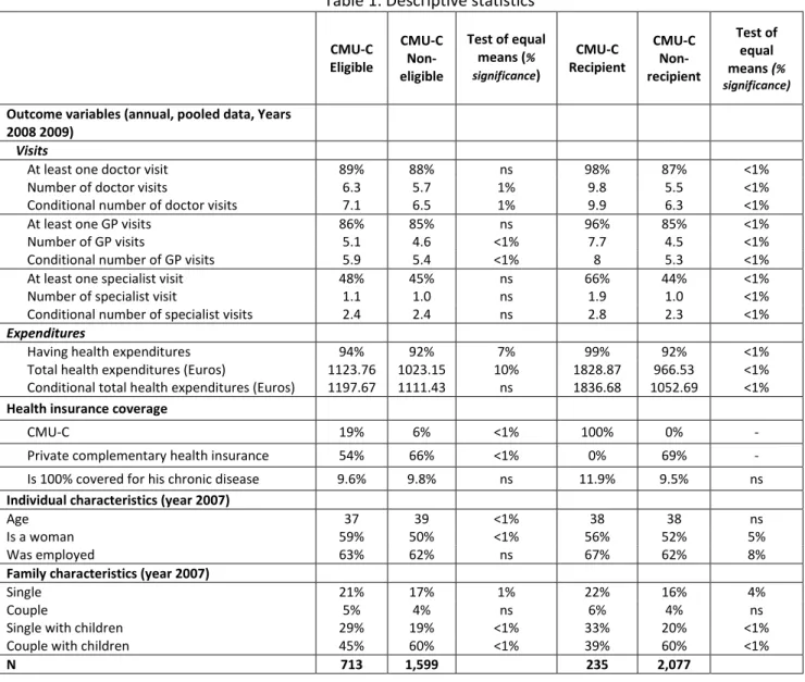
As presented in Table 1, under this definition, 235 (10%) individuals are benefiting from the free plan and given the information on family resources, 713 (31%) individuals are eligible to it. This means that within the CMU-C eligible population, only 20% are covered by the free plan while 54% are covered by a private plan5. Moreover, as previously discussed, due to eligibility measurement errors, 6% of CMU-C non-eligible individuals are actually covered by the free plan.

Table 1 also reports descriptive statistics on healthcare utilisation and individual characteristics. CMU-C eligible individuals use more health services as non eligible individuals. They visit significantly more often a physician, especially general practitioners (GP). They also are more likely to have health expenditures and spend relatively more than non-eligible individuals. These differences are even more accentuated between individuals who benefit from CMU-C and CMU-C non recipients. Regarding their individual and family characteristics, individuals are in average 38 years old. There are slightly more women, single, single and couple with children within the CMU-C eligibles and CMU-C recipients but the proportion of employed individuals is similar and equal to 63% in average. Finally, it is worth noting that 69% of the whole sample is covered by a private complementary health insurance and 10% are fully covered for their chronic disease.

4

In further research, we will have to check the robustness of our results on the definition of this CMU-C variable.

5_{An individual covered at least 6 months in a year by a private health insurance plan was considered as}

(6)

6

Table 1: Descriptive statistics

CMU-C Eligible CMU-C Non-eligible Test of equal means (% significance) CMU-C Recipient CMU-C Non-recipient Test of equal means (% significance)

Outcome variables (annual, pooled data, Years 2008 2009)

Visits

At least one doctor visit 89% 88% ns 98% 87% <1%

Number of doctor visits 6.3 5.7 1% 9.8 5.5 <1%

Conditional number of doctor visits 7.1 6.5 1% 9.9 6.3 <1%

At least one GP visits 86% 85% ns 96% 85% <1%

Number of GP visits 5.1 4.6 <1% 7.7 4.5 <1%

Conditional number of GP visits 5.9 5.4 <1% 8 5.3 <1%

At least one specialist visit 48% 45% ns 66% 44% <1%

Number of specialist visit 1.1 1.0 ns 1.9 1.0 <1%

Conditional number of specialist visits 2.4 2.4 ns 2.8 2.3 <1%

Expenditures

Having health expenditures 94% 92% 7% 99% 92% <1%

Total health expenditures (Euros) 1123.76 1023.15 10% 1828.87 966.53 <1% Conditional total health expenditures (Euros) 1197.67 1111.43 ns 1836.68 1052.69 <1% Health insurance coverage

CMU-C 19% 6% <1% 100% 0% -

Private complementary health insurance 54% 66% <1% 0% 69% -

Is 100% covered for his chronic disease 9.6% 9.8% ns 11.9% 9.5% ns

Individual characteristics (year 2007)

Age 37 39 <1% 38 38 ns

Is a woman 59% 50% <1% 56% 52% 5%

Was employed 63% 62% ns 67% 62% 8%

Family characteristics (year 2007)

Single 21% 17% 1% 22% 16% 4%

Couple 5% 4% ns 6% 4% ns

Single with children 29% 19% <1% 33% 20% <1%

Couple with children 45% 60% <1% 39% 60% <1%

N 713 1,599 235 2,077

4. Estimation strategy

Aim of our study is to estimate the effect of having CMU-C on healthcare utilisation, , (1)

where is the utilisation variable for individual i at time t and a variable indicating whether i is covered by the free plan at the same time. An OLS estimate of equation (1) may be biased because CMU-C is an endogenous variable. CMU-C is correlated with income because access to this coverage is conditioned on income’s level. Even after controlling for income, CMU-C remains endogenous because it is not mandatory. Individuals expecting to use healthcare are more likely to sign up for the free plan.

In order to tackle the endogeneity issue i.e. self-selection issue of health insurance on healthcare utilisation, we use information on the selection rule to qualify for CMU-C and adopt a regression discontinuity approach using eligibility (family income below the cut-off value) as an instrument variable. The principle of this approach is theoretically based on the potential

(7)

7

outcome model, developed by Roy in 1951 and Rubin in 1974. More formally, we are interested in estimating the causal effect of a treatment T “being CMU-C recipient” on an outcome Y “healthcare utilisation”. This model defines two potential outcomes, the outcome of individual i when i is treated and the outcome of individual i when i is untreated. The causal effect of participating in the treatment for i is then equals to = - . But is always unobservable as only one of both outcome variables is observable; when i is treated, is realized and is not observed. is then called the counterfactual outcome and refers to the outcome Y that would have occurred if the individual were treated. We would like to estimate the causal effect of being a CMU-C recipient on healthcare utilisation compares to what it would be if the individual were not covered by the free plan. As the counterfactual is unobservable, aim is to find the best substitute to estimate the causal effect of being CMU-C recipient without bias.

Our identification strategy relies on an assignment variable “family income” that is defined as the family income used for eligibility assessment to CMU-C of individual i at t-1, one year before CMU-C application. Individual i can only qualify for CMU-C if its family income is below the CMU-C cut-off, . We define the dummy variable indicating whether individual i is eligible to CMU-C at time t as Since the free plan is not mandatory, there is no complete compliance between CMU-C eligible individuals and CMU-C recipient individuals ( ). Consequently, we implement a regression discontinuity analysis within a “fuzzy” design.

Formally and as shown by [Hahn et al., 2001 ; Imbens and Lemieux, 2008; Lee and Lemieux 2010], the coefficient b in equation (1) can then be estimated without bias as:

Where b is then the difference between the outcome variable of eligible individuals just below the threshold and the outcome variable of non-eligible individuals just above the threshold. This difference divided by the difference of the outcome variable between CMU-C recipients and CMU-C non recipients around the threshold c.

This estimation relies on three assumptions. First, individuals are unable to manipulate their income in order to become eligible to the free plan so that the effect of being CMU-C recipients is independent of the family income around the threshold. We can imagine that some individuals could choose not to work in order to keep their eligibility to the free plan (the more healthcare is needed). However, it is unlikely that many of them could finally manipulate their income just around the threshold because it supposes that they are able to precisely choose the number of hours worked.

Second, the assignment variable has a discontinuous impact on the probability of being CMU-C recipient. Third, there is a monotonic relationship between CMU-C coverage and eligibility around the threshold. These two last assumptions appear to be given by construction as individuals with family income above the threshold cannot benefit from the free plan. It is actually not precisely the case because we observe income with error. Thus, it means that

(8)

8 .6

We then need to test that we observe family income with enough precision, i.e that these assumptions are both empirically verified.

If these assumptions hold, this approach can then be viewed as a local randomised experiment since the eligibility rule is exogenously given. Therefore, to estimate b we would ideally non-parametrically compare the outcome variable of interest for people below and above the threshold in a small interval. The income bandwidth of our sample is unfortunately too large to assume that income has no significant influence on health utilisation outcomes (independently of the eligibility effect) (i) and that individual characteristics are precisely the same for eligible and non eligible populations (ii). Furthermore our sample is too small to allow narrowing the family income bandwidth.

We then choose to follow the parametric strategy introduced by van der Klaauw in 2002 in order to estimate b, and implement a two-stage estimation as,

where ( ) is a polynomial function of order g of family income and and are unobserved error components. Substituting the equation (2) determining the CMU-C status into the outcome equation (1) yields the reduced form:

where . is then the “intention to treat effect”. Given that the same order of polynomial is used in equation (2) and (3), the effect of the free plan on healthcare utilisation is then identified by the ratio: that is numerically equivalent to the estimate of the two-stage estimate of equation (1) and (2). Put differently, the dummy variable of CMU-C eligibility is used as “instrument” to estimate without bias the effect of being CMU-C recipients on healthcare utilisation [Hahn et al., 2001]. Nevertheless, within a regression discontinuity approach the “instrument” i.e. the eligibility variable does not have to be independent from the outcome variable. It is worth noting that using this two-state procedure, we are in fact estimating a local average treatment effect (LATE) for individuals around the threshold, that is the effect of being CMU-C recipient on healthcare utilisation for “compliers” i.e. on individuals that would choose to be covered by CMU-C if they were eligible to it [Angrist at al., 1996; Imbens and Lemieux, 2008; Lee and Lemieux, 2010]

.

We observe the selection variables to CMU-C (family income and the family size) for the year 2007 (2008) and estimate the effect on outcome variables for the year 2008 (2009). Estimates are run on the pooled dataset and with different bandwidths in order to check the robustness of our results. The baseline specification is a polynomial of order two of the log of family income7, the

6_{Barrow et al., 1980 showed that if the assignment rule is not perfectly known so that the error}

component is not independent from the assignment variable, estimation of equation 1 could lead

to biased estimates.

7_{Best specification using the Akaike information criterion (AIC) as in Lee and Lemieux, 2010. See}

(9)

9

number of individuals in the family, a year dummy for t=2008 and an individual effect in the error component.

5. Results

5.1 Regression discontinuity: Validity check

As presented previously, in order to identify the causal effect of being CMU-C recipients on healthcare utilisation within a fuzzy design, one assumption is to observe a discontinuity of the probability of being CMU-C recipients over the assignment variable (family income) around the threshold.

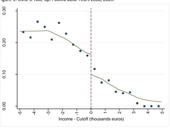
Figure 1 plots the proportion of persons covered by CMU-C over the family income for the years 2008 and 2009. Each dot is the percentage of CMU-C recipients within a family income bin of one thousand Euros width. The solid line is the corresponding local linear smooth plot. We see a clear discontinuity of the proportion of CMU-C recipients around the CMU-C eligibility cut-off point (normalized to zero).

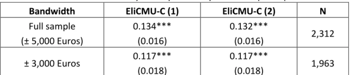
This discontinuity is confirmed by estimates of the probability of CMU-C participation as specified in equation 2 (see table 2). The impact of eligibility (measured by the dummy variable

EliCMUC) on the CMU-C participation is significant and controlling by other explicative variables

does not modify the estimates.

Figure 1: CMU-C Take-up. Pooled data. Years 2008, 2009.

0 .0 0 0 .1 0 0 .2 0 0 .3 0 C MU C Pa rt ici p a ti o n (% ) -5 -4 -3 -2 -1 0 1 2 3 4 5

(10)

10

Table 2: Discontinuity in the probability of CMU-C participation.

Bandwidth EliCMU-C (1) EliCMU-C (2) N

Full sample (± 5,000 Euros) 0.134*** (0.016) 0.132*** (0.016) 2,312 ± 3,000 Euros 0.117*** (0.018) 0.117*** (0.018) 1,963

Note: (1) All regressions are linear probability models including polynomial of order two of the log of family income, the number of individuals in the family, a year dummy for 2008 and an individual effect in the error component. (2) All regressions are linear probability models including polynomial of order two of the log of family income, the number of individuals in the family, a year dummy for 2008, an individual effect in the error component, individual and family characteristics, and a dummy indicating if individual is 100% covered for his chronic disease. Robust standard errors are in brackets.

Statistical significance levels: * 10%; ** 5%; *** 1%.

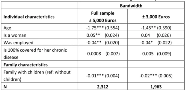
Another assumption that has to be checked is the equal distribution of baseline characteristics or characteristics that are not taken into account in the eligibility assessment around the threshold. This assumption warrants the “local” randomisation quality. We noted in table 1 that eligible and non-eligible individuals to CMU-C are not fully identical. The eligible population appears to be younger, with more women, and with more single family with children. Table 3 reports estimates of the regressions of these individual characteristics on eligibility controlling by family income and family size. We see that eligibility still has a significant influence even if it decreases with the bandwidth size around the threshold. These results suggest that we need to control the estimations of equation 1 and 2 with gender, family composition and employment status in order to ensure that the effect of eligibility on healthcare utilisation is not driven by family characteristics.

However, we assume that individuals cannot precisely manipulate their family income and family size in order to become eligible to CMU-C given the relative complexity of the eligibility rule.

(11)

11

Table 3: Balance of controls around the threshold (pooled data) Bandwidth

Individual characteristics Full sample

± 5,000 Euros ± 3,000 Euros

Age -1.75*** (0.554) -1.45** (0.590)

Is a woman 0.05** (0.024) 0.04 (0.026)

Was employed -0.04** (0.020) -0.04* (0.022)

Is 100% covered for her chronic

disease -0.0008 (0.007) -0.005 (0.009)

Family characteristics

Family with children (ref: without

children) -0.01*** (0.004) -0.02*** (0.005)

N 2,312 1,963

Note: Each estimate is the coefficient of the dummy variable EliCMUC in estimations of equation 2, the explained variable being replaced by individual and family characteristics. All Regressions are linear probability models (except for age, we estimated a linear model) including polynomial of order two of the log of family income, the number of individuals in the family, a year dummy for 2008 and an individual effect in the error component. Robust standard errors are in brackets. Statistical significance levels: * 10%; ** 5%; *** 1%.

5.2 Impact of the free plan on healthcare utilisation

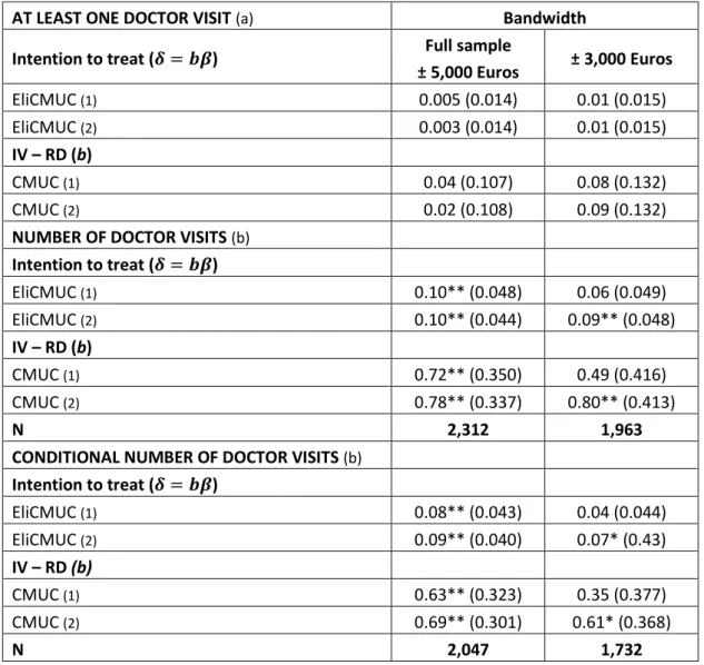
Tables 4, 5 and 6 display estimates of parameters (intention to treat) and b of equation (1) and (3) for different healthcare utilisation outcomes: doctor visits, GP visits, specialist visits and total health expenditures. Estimates are displayed for two bandwidths and with (without) controlling for family characteristics.

We firstly observe that estimates are very similar for the two bandwidths when controlling by family characteristics. It is not the case without controls. This likely means that with narrow bandwidth we lose in precision concerning eligibility measurement and that controlling with family characteristics improves the eligibility measurement accuracy.

The likelihood of visiting a doctor is not impacted by CMU-C. This is not really surprising because a very large majority of individuals in the sample visits a doctor at least one time in a year (table 1). On the other hand the number of visits is significantly higher for people with CMU-C. The number of doctor visits is twice higher for people covered by the free plan (table 4). This is roughly what we observe in the descriptive statistics (table 1).

(12)

12

Table 4: Impact of the free plan on doctor visits

AT LEAST ONE DOCTOR VISIT (a) Bandwidth

Intention to treat ( ) Full sample

± 5,000 Euros ± 3,000 Euros EliCMUC (1) 0.005 (0.014) 0.01 (0.015) EliCMUC (2) 0.003 (0.014) 0.01 (0.015) IV – RD (b) CMUC (1) 0.04 (0.107) 0.08 (0.132) CMUC (2) 0.02 (0.108) 0.09 (0.132)

NUMBER OF DOCTOR VISITS (b)

Intention to treat ( ) EliCMUC (1) 0.10** (0.048) 0.06 (0.049) EliCMUC (2) 0.10** (0.044) 0.09** (0.048) IV – RD (b) CMUC (1) 0.72** (0.350) 0.49 (0.416) CMUC (2) 0.78** (0.337) 0.80** (0.413) N 2,312 1,963

CONDITIONAL NUMBER OF DOCTOR VISITS (b)

Intention to treat ( ) EliCMUC (1) 0.08** (0.043) 0.04 (0.044) EliCMUC (2) 0.09** (0.040) 0.07* (0.43) IV – RD (b) CMUC (1) 0.63** (0.323) 0.35 (0.377) CMUC (2) 0.69** (0.301) 0.61* (0.368) N 2,047 1,732

Note: (a) All regressions are linear probability models. (b) All regressions are negative binomial models; Marginal effects of the number of visits are then given by the exponential of the displayed coefficient. Regressions in (1) include polynomial of order two of the log of family income, the number of individual in the family, a year dummy for 2008 and an individual effect in the error component. Regressions in (2) polynomial of order two of the log of family income, the number of individual in the family, a year dummy for 2008, individual effect in the error component, individual and family characteristics, and a dummy indicating if individual is 100% covered for his chronic disease. Robust standard errors are in brackets. Statistical significance levels: * 10%; ** 5%; *** 1%.

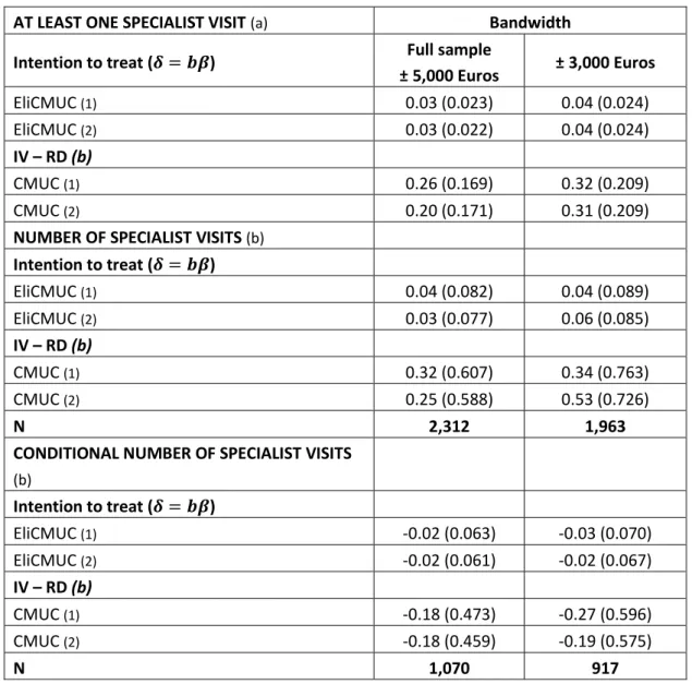
Looking at the effect of CMU-C on visits to the GP and on visits to the specialist separately, we see that the effect on doctor visits is mainly driven by visits to the GP. Again the likelihood of seeing a GP or a specialist is positive but not significantly different from zero. The number of visits to a GP is twice as great for CMU-C recipients as for non recipients (table 5). However, the free plan seems to have no impact on the number of specialist visits (table 6). We note here that the difference observed on descriptive statistics withdraws after controlling for endogeneity. Several reasons may explain this result. Individuals visiting specialists are mainly those who suffer from a chronic disease. CMU-C recipients may also forego seeing a specialist because they are experiencing treatment refusals [Després & Couralet, 2011

]

.

(13)

13

Table 5: Impact of the free plan on GP visits

AT LEAST ONE GP VISIT (a) Bandwidth

± 5,000 Euros ± 3,000 Euros EliCMUC (1) 0.006 (0.016) 0.01 (0.017) EliCMUC (2) 0.002 (0.016) 0.009 (0.017) IV - RD CMUC (1) 0.04 (0.118) 0.09 (0.149) CMUC (2) 0.02 (0.119) 0.08 (0.148) NUMBER OF GP VISITS (b) Intention to treat ( ) EliCMUC (1) 0.10** (0.047) 0.07 (0.049) EliCMUC (2) 0.11** (0.046) 0.10** (0.049) IV - RD CMUC (1) 0.78** (0.358) 0.56 (0.419) CMUC (2) 0.87** (0.346) 0.86** (0.419) N 2,312 1,963

CONDITIONAL NUMBER OF GP VISITS (b)

Intention to treat ( ) EliCMUC (1) 0.08** (0.043) 0.04 (0.044) EliCMUC (2) 0.10** (0.039) 0.07* (0.043) IV – RD (b) CMUC (1) 0.64** (0.323) 0.37 (0.37) CMUC (2) 0.75** (0.302) 0.64* (0.363) N 1,984 1,676

Note: (a) All regressions are linear probability models. (b) All regressions are negative binomial models; Marginal effects of the number of visits are then given by the exponential of the displayed coefficient. Regressions in (1) include polynomial of order two of the log of family income, the number of individual in the family, a year dummy for 2008 and an individual effect in the error component. Regressions in (2) polynomial of order two of the log of family income, the number of individual in the family, a year dummy for 2008, an individual effect in the error component, individual and family characteristics, and a dummy indicating if individual is 100% covered for his chronic disease. Robust standard errors are in brackets. Statistical significance levels: * 10%; ** 5%; *** 1%.

(14)

14

Table 6: Impact of the free plan on specialist visits

AT LEAST ONE SPECIALIST VISIT (a) Bandwidth

NUMBER OF SPECIALIST VISITS (b)

Intention to treat ( ) EliCMUC (1) 0.04 (0.082) 0.04 (0.089) EliCMUC (2) 0.03 (0.077) 0.06 (0.085) IV – RD (b) CMUC (1) 0.32 (0.607) 0.34 (0.763) CMUC (2) 0.25 (0.588) 0.53 (0.726) N 2,312 1,963

CONDITIONAL NUMBER OF SPECIALIST VISITS (b) Intention to treat ( ) EliCMUC (1) -0.02 (0.063) -0.03 (0.070) EliCMUC (2) -0.02 (0.061) -0.02 (0.067) IV – RD (b) CMUC (1) -0.18 (0.473) -0.27 (0.596) CMUC (2) -0.18 (0.459) -0.19 (0.575) N 1,070 917

Note: (a) All regressions are linear probability models. (b) All regressions are negative binomial models; Marginal effects of the number of visits are then given by the exponential of the displayed coefficient. Regressions in (1) include polynomial of order two of the log of family income, the number of individual in the family, a year dummy for 2008 and an individual effect in the error component. Regressions in (2) polynomial of order two of the log of family income, the number of individual in the family, a year dummy for 2008, an individual effect in the error component individual and family characteristics, and a dummy indicating if individual is 100% covered for his chronic disease. Robust standard errors are in brackets. Statistical significance levels: * 10%; ** 5%; *** 1%.

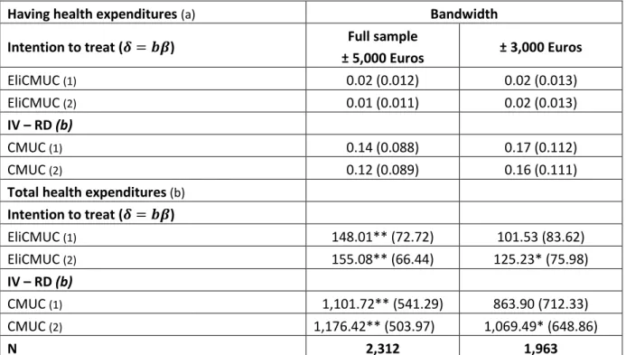
Concerning total health expenditures, individuals with CMU-C coverage spend much more than individuals not covered by CMU-C: more than 1,000 Euros per year (conditionally to have health expenditures during the year) near the average health expenditures and slightly higher than the difference in health expenditures between CMU-C recipients and non recipients (see table 1). In other words, controlling for the endogeneity of CMU-C does not deeply modify the difference observed in the descriptive statistics between CMU-C recipients and non recipients.

(15)

15

These results show that the free plan has a large impact on healthcare utilisation of poor individuals just above and just below the CMU-C income threshold. Nevertheless, it is not really the access to health care system which is involved but more precisely the use of healthcare services given that the probability to visit a doctor is not significantly higher for CMU-C recipients. It is then difficult to conclude whether the higher utilisation of health care services of the CMU-C recipients is induced by physicians (taking into account the cost of their patients‘health services) or by the demand of the insured persons themselves.

Table 7: Impact of the free plan on total health expenditures

Having health expenditures (a) Bandwidth

Total health expenditures (b)

Intention to treat ( ) EliCMUC (1) 148.01** (72.72) 101.53 (83.62) EliCMUC (2) 155.08** (66.44) 125.23* (75.98) IV – RD (b) CMUC (1) 1,101.72** (541.29) 863.90 (712.33) CMUC (2) 1,176.42** (503.97) 1,069.49* (648.86) N 2,312 1,963

Note: (a) All regressions are linear probability models. (b) All regressions are tobit models. Regressions in (1) include polynomial of order two of the log of family income, the number of individual in the family, a year dummy for 2008 and an individual effect in the error component. Regressions in (2) polynomial of order two of the log of family income, the number of individual in the family, a year dummy for 2008, an individual effect in the error component, individual and family characteristics, and a dummy indicating if individual is 100% covered for his chronic disease. Robust standard errors are in brackets. Statistical significance levels: * 10%; ** 5%; *** 1%.

(16)

16 6. Discussion

The impact of CMU-C on healthcare access and health expenditures for poor individuals around the eligibility income threshold is difficult to analyse because all eligible individuals are not covered by the free plan. A direct comparison of healthcare outcomes of CMU-C recipients and non-recipients, just above and just below the threshold, is not relevant due to the selection mechanism involved: CMU-C recipients are individuals who likely need more healthcares. This comparison (table 1) shows very large and significant differences between CMU-C recipients and non-recipients for every type of healthcare outcomes (visit to doctor, health expenditures) while a large part of the non-recipients are covered by a private complementary health insurance plan. The issue is to ensure that these differences are not due to the self-selection of CMU-C recipients.

In order to tackle this endogeneity issue, we used information on the selection rule to qualify for the free plan and adopt a regression discontinuity approach using eligibility (family income below the cut-off value) as an instrument variable. The observed differences on health care utilisations in descriptive statistics are confirmed by the estimates controlling for potential selection bias. CMU-C recipients visit significantly more a physician and spend significantly more on healthcare. Nevertheless, access to the healthcare system measured as the likelihood of visiting a doctor or of spending money on healthcare appears not to be significantly influenced by the free plan. It is worth noting that these results are obtained even though a majority of non eligible individuals are covered by a private plan. This means that the eligibility threshold has on

average an impact on health care expenditures and on the number of visits. Obviously, part of this

impact is due to the fact that some of the non eligible individuals choose to remain uncovered. Despites this fact, CMU-C seems to generate significant inequities in healthcare utilisation.

In further research, it would be interesting to compare healthcare utilisation of CMU-C recipients to healthcare utilisation of individuals covered by a private plan on the one hand and to healthcare utilisation of uncovered individuals on the other hand. However, we would be additionally confronted with the endogeneity issue of the private plan in the same way as for the free plan; Therefore, we would need another valid instrument to control for the endogeneity of the private plan variable.

Since we do not perfectly observe the family income used to assess eligibility to the free plan and therefore the actual CMU-C eligibility, we will have to tackle this issue more explicitly. As shown by Battistin et al. in 2009 and also implemented by Hullegie et al. in 2010 this could result in a smooth link between income and the probability to be covered by the free plan around the threshold and could then invalid the discontinuity regression approach followed in this paper. We will have to deal with this issue following the method developed by these authors. Finally, we would like to implement non parametrical methods and control for the observed heterogeneity between eligible individuals and non eligible individuals in order to test the robustness of our results.

(17)

17 References:

Angrist JD, Imbens GW, Rubin DB. 1996. Identification of causal effects using instrumental variables. Journal of the American Statistical Association. 91: 444-472.

Barnow BS, Cain GG, Goldberger AS. 1980. Issues in the Analysis of Selectivity Bias in E. Stormsdorfer and G. Farkase ds., Evaluation Studies, 5: 43-59 (Beverly Hills: Sage Publications) Battistin E, Brugiavini A, Rettore E, Weber G. 2009. The retirement consumption puzzle: evidence from a regression discontinuity approach. American Economic Review. 99 : 2209 – 2226.

Buchmueller TC, Couffinhal A, Grignon M, Perronnin M. 2004. Access to physician services: does supplemental insurance matter? Evidence from France. Health Economics. 13: 669–687.

Code de la Sécurité Sociale. 2011. Articles R. 861-1 à 10, articles R. 861-16 à 18. http://www.legifrance.gouv.fr/

Card D, Shore-Sheppard LD. 2004. Using Discontinuous Eligibility Rules to Identify the Effects of the Federal Medicaid Expansions on Low-Income Children. Review of Economics and Statistics. 86(3): 752–766.

Card D, Dobkin C, Maestas N. 2008. The Impact of Nearly Universal Insurance Coverage on Health Care Utilization: Evidence from Medicare. American Economic Review. 98(5) 2242 – 2258.

Card D, Dobkin C, Maestas, N. 2009. Does Medicare Save Lives?. Quarterly Journal of Economics. 124(2): 597 – 636

Caussat L, Glaude M. 1993. Dépenses médicales et couverture sociale. Economie et statistique. 265: 31-43.

Chiappori PA, Durand F, Geoffard PY. 1998. Moral Hazard and the demand for physician services: First lessons from a French natural experiment. European Economic Review. 42: 499-511.

De la Mata D. 2011. The effect of Medicaid on children’s health: a regression discontinuity approach. Working paper presented to the Twentieth European workshop on econometrics and health economics, York, 7-10 September.

Després C, Couralet PE. 2011. Situation testing: The case of health care refusal. Revue

d'Épidémiologie et de Santé Publique. 59(2) : 77-89.

Fonds CMU. 2011a. Plafonds applicables pour l'octroi de la CMU complémentaire et de l’aide complémentaire santé. http://www.cmu.fr/userdocs/232-2-2011v3.pdf.

(18)

18

Fonds CMU. 2011b. L'attribution de la CMU complémentaire. http://www.cmu.fr/userdocs/2112-1_2010.pdf.

Fonds CMU, 2011c. Bénéficiaires de la CMU complémentaire en France entière. Mise en ligne le 27.06.2011 sur le site du fonds CMU http://www.cmu.fr.

Genier P. 1998. Assurance et recours aux soins. Une analyse microéconométrique à partir de l’enquête Santé 1991- 1992 de l’Insee. Revue économique. 49(3): 809-819.

Grignon M, Perronnin M, Lavis JN. 2008. Does free complementary health insurance help the poor to access health care? Evidence from France. Health Economics. 17(2): 203-219.

Hahn J, Todd P, Van der Klaauw W. 2001. Identification and Estimation Effects with a Regression-Discontinuity Design. Econometrica. 69(1): 201-209.

Hullegie P, Klein TJ. 2010. The effect of private health insurance on medical care utilization and self-assessed health in Germany. Health Economics. 19: 1048–1062.

Imbens GW, Lemieux T. 2008. Regression discontinuity designs: A guide to practice. Journal of

Econometrics. 142(2): 615-635.

Lee DS, Lemieux T. 2010. Regression Discontinuity Designs in Economics. Journal of Economic Literature. 48: 281-355.

Mormiche P. 1993. Les disparités de recours aux soins en 1991. Economie et statistique. 265: 45-52.

Roy AD. 1951. Some Thoughts on the Distribution of Earnings. Oxford Economic Papers, New

Series. 3(2):135-146.

Rubin DB. 1974. Estimating causal effects of treatments in randomized and nonrandomized studies. Journal of Educational Psychology. 66(5):688-701.

Thistlethwaite DL, Campbell DT. 1960. Regression-Discontinuity Analysis: An Alternative to the Ex Post Facto Experiment. Journal of Educational Psychology. 51(6): 309-17.

Van der Klaauw W. 2002. Estimating the Effect of Financial Aid Offers on College Enrollment: A Regression-Discontinuity Approach. International Economic Review. 43(4): 1249-1287.

(19)

19

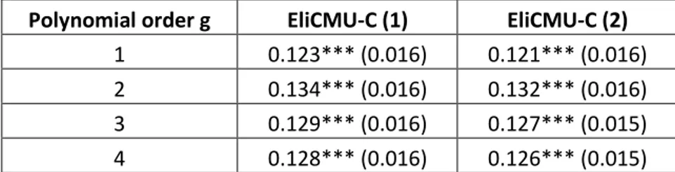
Appendix A: Sensitivity analysis of the model specification

Table A.1 reports the estimates of equation: , where ( ) is a polynomial function of order g of family income and and are unobserved error components. We test the robustness of our results for different polynomial order of the log of family income.

Table A.1: Sensibility of the discontinuity point

Polynomial order g EliCMU-C (1) EliCMU-C (2)

1 0.123*** (0.016) 0.121*** (0.016) 2 0.134*** (0.016) 0.132*** (0.016) 3 0.129*** (0.016) 0.127*** (0.015) 4 0.128*** (0.016) 0.126*** (0.015) Note: (1) All regressions are linear probability models including polynomial of order g of the log of family income, the number of individuals in the family, a year dummy for 2008 and an individual effect in the error component. (2) All regressions are linear probability models including polynomial of order g of the log of family income, the number of individuals in the family, a year dummy for 2008, an individual effect in the error component, individual and family characteristics, and a dummy indicating if individual is 100% covered for his chronic disease. Robust standard errors are in brackets.

Statistical significance levels: * 10%; ** 5%; *** 1%.

Tables A.2, A.3, A.4 and A.5 report the estimates of equation: , where ( ) is a polynomial function of order g of family income and and are unobserved error components. We test the robustness of our results for different polynomial order of the log of family income. We displayed results for the number of visits, the number of GP visits, the number of specialist visits and the total expenditures. The sensitivity analysis for the other outcome variables are available upon request.

(20)

20

Table A.2: Sensibility of the “intention to treat effect” for the number of visits

1 0.08* (0.046) 0.09** (0.044)

2 0.10** (0.048) 0.10** (0.044)

3 0.09** (0.047) 0.10** (0.044)

4 0.09** (0.047) 0.10** (0.044)

Note: All regressions are negative binomial models; Marginal effects of the number of visits are then given by the exponential of the displayed coefficient. Regressions in (1) include polynomial of order g of the log of family income, the number of individual in the family, a year dummy for 2008 and an individual effect in the error component. Regressions in (2) polynomial of order g of the log of family income, the number of individual in the family, a year dummy for 2008, an individual effect in the error component, individual and family characteristics, and a dummy indicating if individual is 100% covered for his chronic disease. Robust standard errors are in brackets. Statistical significance levels: * 10%; ** 5%; *** 1%.

Table A.3: Sensibility of the “intention to treat effect” for the number of GP visits

1 0.09* (0.047) 0.10** (0.045)

2 0.10** (0.047) 0.11** (0.046)

3 0.10** (0.047 0.11** (0.045)

4 0.10** (0.048) 0.11** (0.045)

(21)

21

Table A.4: Sensibility of the “intention to treat effect” for the number of specialist visits

1 0.03 (0.081) 0.02 (0.077)

2 0.04 (0.082) 0.03 (0.077)

3 0.04 (0.081) 0.03 (0.077)

4 0.04 (0.081) 0.03 (0.076)

Table A.5: Sensibility of the “intention to treat effect” for the total expenditures

1 137.14* (72.02) 145.88** (65.73)

2 148.01** (72.72) 155.08** (66.44) 3 143.11** (71.92) 150.51** (65.63) 4 142.79** (71.91) 150.14** (65.62) Note: All regressions are tobit models. Regressions in (1) include polynomial of order g of the log of family income, the number of individual in the family, a year dummy for 2008 and an individual effect in the error component. Regressions in (2) polynomial of order g of the log of family income, the number of individual in the family, a year dummy for 2008, an individual effect in the error component, individual and family characteristics, and a dummy indicating if individual is 100% covered for his chronic disease. Robust standard errors are in brackets. Statistical significance levels: * 10%; ** 5%; *** 1%.