A Comparison of the Poverty Impact of Transfers, Taxes and Market Income across five OECD Countries

(1)

Bibi : CIRPÉE, Pavillon DeSève, Université Laval, Québec, Canada G1K 7P4; Phone: 1-418-656-2131 ext. 13246 Fax: 1-418-656-7798

sbibi@ecn.ulaval.ca

Duclos : Department of economics and CIRPÉE, Pavillon DeSève, Université Laval, Québec, Canada G1K 7P4; Phone: 1-418-656-7096; Fax: 1-418-656-7798

jyves@ecn.ulaval.ca

This research is funded in part by Quebec’s FQRSC and by the Poverty and Economic Policy international research network. We are grateful to Bernard Fortin, Guy Lacroix, Simon Langlois and François Blais for their helpful comments and suggestions.

Cahier de recherche/Working Paper 08-35

A Comparison of the Poverty Impact of Transfers, Taxes and Market

Income across Five OECD Countries

Sami Bibi

Jean-Yves Duclos

(2)

Abstract:

This paper compares the poverty reduction impact of income sources, taxes and transfers across five OECD countries. Since the estimation of that impact can depend on the order in which the various income sources are introduced into the analysis, it is done by using the Shapley value. Estimates of the poverty reduction impact are presented in a normalized and un-normalized fashion, in order to take into account the total as well as the per dollar impacts. The methodology is applied to data from the Luxembourg Income Study (LIS) database.

Keywords: Poverty reduction, Transfers, Taxes, Shapley Value; OECD Countries

(3)

1 Introduction

Most OECD countries devote a substantial share of public resources to social transfers in order to redistribute income and reduce poverty. To assess the poverty effectiveness of such social transfers, it is usual to compute the change in poverty that they induce. In order to do this, a benchmark of pre-transfer income is first defined; the distributional impact of social transfers is then estimated as the fall in poverty estimated following the addition of the transfers, with or without the presence of behavioral responses. The poverty effectiveness of the transfers in alleviating poverty can also be computed per dollar of transfer.

A problem arises, however, in evaluating the impact of a set of social trans-fers that operate simultaneously. The order in which the transtrans-fers are ranked can indeed influence the estimates of the poverty reduction effect attributed to each individual transfer in the set. To illustrate this, consider the case of a country with two identical universal transfers. Assume that each transfer awards everyone a transfer equal to the poverty line (regardless of his/her income), so that no person is poor after the implementation of any of the two. If the benchmark income used to estimate the poverty effectiveness of one transfer includes the other transfer, none of the transfer will show any impact on poverty, albeit both lead to a total eradication of poverty when the other program is not included in the benchmark income. Since it usually arbitrary to prefer one order to the other, it would seem useful to think of a sharing rule that assigns each transfer a poverty impact that

does not depend on the ranking of the various income sources. 1

The paper proposes such a rule by importing from cooperative game theory the use of the Shapley value. The procedure can be used for positive (transfers, earnings, capital income, etc.) or negative sources of income (such as income taxes). The paper also computes the effect of income sources across wide ranges of poverty lines and for broad classes of poverty indices in order to address the difficult of selecting “one” poverty line.

The paper then studies the poverty effects of a comparable set of social trans-fers that are in force in five OECD countries. Comparing national experiences on social transfers and poverty alleviation effects may provide useful policy guid-ance on alternative means of achieving social objectives. Social transfers differ both in terms of their scale and in terms of their distribution. Scale matters for the total change in poverty induced by a social transfer; distribution relates to the 1_{See for instance, Smeeding (2006), who computes the poverty impact of social insurance and}

(4)

effectiveness of poverty alleviation per dollar of transfer spent. Further, due to the size effect of the different income sources, their effectiveness in reducing poverty is measured using an indicator which weighs up the scale and the distribution of each income source.

The paper uses data on five OECD countries drawn from the Luxembourg

Income Study (LIS) (http://www.lisproject.org), each with a recent 1999-2000

LIS database. They are Canada, United States, United Kingdom, Germany, and Sweden. The choice of these countries is based both on the availability of data and on the presence of similar national welfare programs across them.

The rest of the paper is structured as follows. Section 2 presents the poverty lines and the poverty measures. Section 3 describes the sharing rule used to esti-mate the scale and the distribution of the poverty impact of different social trans-fers. Section 4 applies the methodology to five OECD countries with similar tax and transfer systems. Section 5 concludes.

2 Poverty

How poverty is defined and measured is important for understanding poverty; it is also important for understanding the effectiveness of poverty alleviation pro-grams. One influential definition of poverty is that it exists when one or more persons fall short of a level of consumption of goods and services deemed to con-stitute a reasonable minimum, either in some absolute sense or by the standards of a specific society Lipton and Ravallion 1995. This, however, usually involves the selection of one or a few arbitrary poverty lines. To guard against this degree of arbitrariness, the paper will compare the impact of income sources over wide ranges of poverty lines (see Section 4.2).

Note that this paper will use absolute poverty lines. With relative poverty lines, a social transfer that raises the incomes of all, but proportionally more those of the non-poor, may worsen poverty, albeit the absolute income of the poor has increased. Conversely, a progressive tax income that decreases everyone’s income but proportionally more that of the non-poor, will reduce poverty, although the absolute income of the poor falls.

There is also the issue of which poverty index to use to estimate the effective-ness of redistributive policies. The most popular poverty index is the incidence of poverty, namely, the proportion of the population living with less than the poverty line. It has often been criticized (see for instance Sen (1976)) for only capturing the changes in the proportion of the population that is poor, and not capturing

(5)

the changes in the well-being of the poor. Moreover, most anti-poverty welfare programs are often not designed to lift the poor entirely out of poverty; they do, however, purport to improve their living standards. This may not be adequately captured by the use of the poverty headcount.

Instead of just one index at one poverty line, we will use indices that are mem-bers of the popular (Foster, Greer, and Thorbecke 1984) (FGT) family of poverty indices over ranges of poverty lines. Let z be a real poverty line. The FGT indices are defined as Pα(y, z) = 100 Z _z 0 µ z − x z ¶_α dFy(x), (1)

where Fy(x) is the cumulative distribution function of income y. α is a “poverty

aversion” parameter; it captures the sensitivity of the index to changes in the

dis-tribution2_{. As is well known, P}

0(y, z) is the incidence of poverty (the headcount

ratio), P1(y, z) is the normalized average poverty gap measure (the “intensity” of

poverty), and P2(y, z) is often described as an index of the “severity” of poverty

– it weights poverty gaps by poverty gaps. For α > 1, Pα(y, z) is sensitive to the

distribution of incomes among the poor, and when α becomes very large, Pα(y, z)

approaches a Rawlsian measure (Rawls 1971).

3 Impact of income sources on poverty

3.1 The Shapley value

Consider T income sources, including market income, transfers (social secu-rity, welfare, child benefits, etc.), and taxes. These income sources impact simul-taneously on total income and individual poverty; we wish, however, to infer their separate contribution to total poverty reduction, in order for instance to determine which ones are more cost effective in redistributing income and reducing poverty. To do this, we consider a rule based on the Shapley value. First, we need to specify a baseline situation, which we assume to be given by the distribution in which the income of everyone is nil. From (1), this means that initial poverty is equal to 100 regardless of the value of α. Suppose now that the T sources of income are ordered in a certain way. The poverty reduction due to the first source of income, market income say, is computed assuming that it is the unique

(6)

source of income; 100 minus the level of poverty with market income is then the contribution of market income to poverty alleviation. Next, the additional fall in poverty owing to the second source, social security say, is calculated by adding social security to market income. This pattern is repeated until total poverty re-duction – achieved through total income – is allocated across the various income components.

The above is sometimes called an “incremental benefit” allocation procedure. It uses just one of the many possible orders in which income sources can be ranked. There is usually no ethical or other justification for a particular given or-dering. An order also generally “overestimates” the contribution to overall poverty reduction of the income source that is included first in the ordering, and underes-timates the contribution of the income source included last.

The Shapley value can help address such concerns. Let Y be the set of all

income sources yi, i = 1, ..., T , including negative ones such as income taxes.3

Some income sources may be grouped to form a subset S of Y (S ⊆ Y ). Define

Si as a subset of Y that does not include yi, i.e., Si ⊆ Y \{yi}, and πα(Si, z) as

a characteristic function that satisfies πα(∅, z) = 0, where ∅ is the empty set. For

a subset Si, πα(Si, z) is the contribution of the welfare elements included in Sito

total poverty reduction ∆Pα(Y, z) = 100 − Pα(Y, z), regardless of the effect that

any yi external to Simay have. Since some elements of Simay contribute more to

πα(Si, z) than others, the question arises as to how to distribute πα(Si, z) across

the elements of Si. To address this issue, several approaches have been suggested.

The most popular one was introduced by Shapley (1953). It fulfills the following axioms.

Axiom 1 Efficiency: The overall poverty reduction generated by Y is the sum of πα(yi, z), that is, the poverty reduction effected by each income source i:

T

X

i=1

πα(yi, z) = ∆Pα(Y, z) = 100 − Pα(Y, z) = πα(Y, z). (2)

Axiom 2 Symmetry: If yi and yj are symmetric (or perfectly substitutes), i.e.,

πα(Si,j∪ {yi}, z) = πα(Si,j ∪ {yj}, z), then:

πα(yi, z) = πα(yj, z). (3)

3_{The value of these income sources will usually be adjusted for differences in individual needs}

(7)

Axiom 3 Focus: Whenever yi does not change poverty, i.e., πα(Si ∪ {yi}, z) =

πα(Si, z), then:4

πα(yi, z) = 0. (4) Axiom 4 Additivity: The cumulative poverty reduction generated by S is the sum of the poverty reduction effected by each of its components. Or, phrased differ-ently, ∀Si,j ⊆ Y \{yi, yj}, we have:

πα(Si,j ∪ {yi, yj}, z) = πα(Si,j∪ {yi}, z) + πα(yj, z) (5)

= πα(Si,j∪ {yj}, z) + πα(yi, z).

The Shapley value induces an allocation rule πα(.) that allocates to each

in-come source yia weighted mean of the source’s marginal (incremental)

contribu-tion to overall poverty reduccontribu-tion. It is the only allocacontribu-tion rule that satisfies the

axioms listed above. The poverty reduction that yi gets with the characteristic

function πα(.) is: πα(yi, z) = 1 2(T −1)! X R £ Pα ¡ SR i ∪ {yi}, z ¢ − Pα ¡ SR i , z ¢¤ (6)

where R crosses the 2(T −1)!_{possible permutations of Y and S}R

i ⊆ Y \{yi} is the

subset of income sources preceding yi within the order R. Equation (6) clearly

shows that the contribution of an income source yi to overall poverty reduction

is obtained by averaging its marginal contribution over all the possible different

permutations SR

i from which πα(yi, z) can be computed.

3.2 The poverty effectiveness of income sources

We can think of the poverty effectiveness of a social transfer as depending both upon the poverty change it yields and the size of the budgetary cost that it

generates.5 _{Indeed, for policy purposes, it is important to take into account both}

the “benefit” and the “cost” of the use of social transfers for distributive purposes. To integrate the cost and the benefit of redistributive transfers, we may simply

divide the poverty impact of an income source by the size of that source. Let y∗

i

4_{This is the well-known “dummy” axiom in cooperative game theory.}

5_{This distinction is not always made; see for instance Makdissi, Therrien, and Wodon (2006)}

and Smeeding (2006) for comparative studies of the poverty effect of redistributive transfers in Canada and United States.

(8)

be income from source i, (i = 1, ..., T ).6 _{Then, the average of y}∗

i expressed as a

percentage of the absolute poverty line, z, is:

y_i = 100 z Z _+∞ 0 y∗_idF (y∗_i), (7) where F (y∗

i) is the distribution function of income source y∗i. The ratio of πα(yi, z)

to y_iyields Γα(yi, z), the poverty impact of income source i for a value of yiequal

to the poverty line:

Γα(yi, z) = 100δ

πα(yi, z)

y_i , (8)

where δ = 1 or −1 according to whether the income source i is positive or nega-tive.

Comparing Γα(yi, z) across i can help assess which transfers are most effective

in reducing poverty per dollar spent, or which taxes are least costly in terms of

poverty aggravation per dollar generated. 7 _{Whenever Γ}

α(yi, z) > Γα(yj, z), each

dollar spent on program i reduces poverty more on average than that spent on program j.

4 The poverty effectiveness of transfers, taxes and

market income across some OECD countries

The methodology presented above is illustrated using data from the Luxem-bourg Income Study (LIS) for Canada (CA), United States (US), United Kingdom (UK), Germany (DE), and Sweden (SE). For four of these countries, a (relatively) recent 2000 LIS database is available (1999 for the UK). These countries also have

relatively similar tax and transfer systems that feature:8

1. Market Income (MI);

2. Old-age Benefits (OB);

3. Child Benefits (CB);

6_{This will usually be income per person, unlike y}

i, which would usually be adult-equivalent

income.

7_{If y}

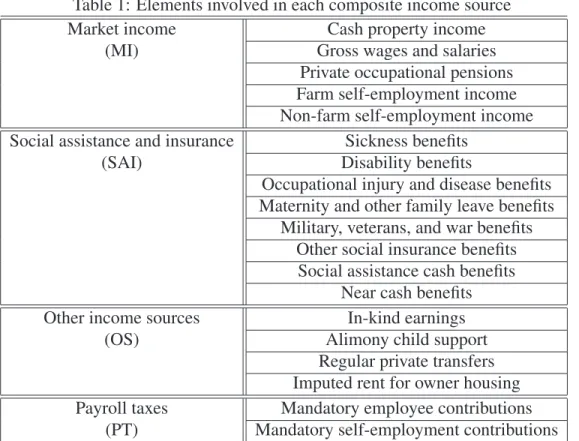
istands for a tax, Γα(yi, z) measures the poverty increase per dollar of tax raised from i. 8_{A detailed content of some of these income sources can be found in Table 1.}

(9)

4. Unemployment Benefits (UB);

5. Social Assistance and Insurance (SAI);

6. Other Income Sources (OS);

7. Income Taxes (IT) ;

8. Payroll Taxes (PT);

9. Other Direct Taxes (OT);

10. Net Income (NI).

To adjust for differences in household composition, we use the OECD-modified equivalence scale proposed by Hagenaars, de Vos, and Zaidi (1994) that assigns a weight of 1 to the household head, of 0.5 to each additional adult, and of 0.3 to each child who is less than 14 years old. To compare poverty across countries, we need a poverty line that represents the same purchasing power across the re-tained countries. For this, we first select the US official (absolute) poverty line and convert it for other countries into specific (absolute) poverty standards using the purchasing power parities (PPP) found in OECD (2005).

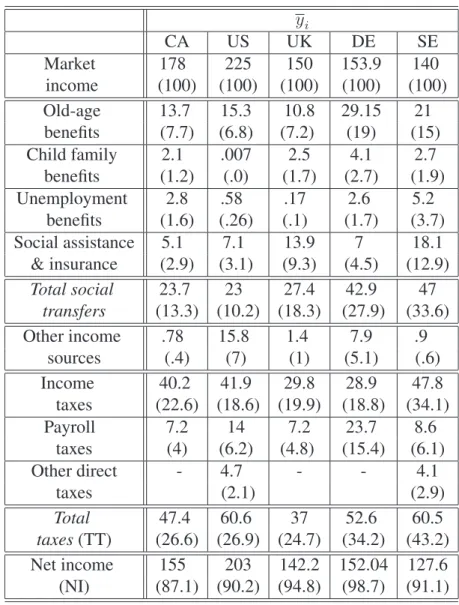
Tables 2 and 3 show some descriptive statistics related to the PPP, the absolute poverty lines in domestic currencies, and the mean of the different income sources across the countries. All of the statistics presented in Table 3 are expressed in percentage of the equivalent of the US official poverty line.

As one may expect, Table 3 shows that market income is the most important income source in the five countries. It ranges from 225 percent of the poverty line (z) in the US to 140 percent of the same poverty standard in Sweden. Market income is followed by old-age benefits, which range from roughly 29 percent of

z in Germany to 11 percent in United Kingdom. The importance of the other

positive income sources varies from one country to another. For instance, social assistance and insurance (beyond unemployment benefits) range from 18 percent of z in Sweden to 5.1 percent in Canada. Sweden and Germany devote by far the highest absolute effort in dollar terms in social transfers, while the United states and, to a lesser extent, Canada spend the least. The united States devotes roughly 10 percent of its total market income in social transfers; this corresponds to roughly half the share of market income spent for the same purpose in the UK, and to about a third of the effort made in Sweden and Germany. Somewhat unsurprisingly, the tax burden is highest in both absolute and relative terms in

(10)

Sweden and Germany, and is lowest in relative terms in United Kingdom, Canada and United States.

4.1 Poverty impact

The impact of the different income sources on poverty incidence and deficit,

π0(yi, z) and π1(yi, z), is displayed in Tables 4 and 5, respectively. As expected,

the poverty impact by income source is largely correlated with the share of the source in total income. Thus, the largest income source, market income, con-tributes most to lowering the incidence and the deficit of poverty, whereas several social transfers contribute absolutely little to overall poverty reduction. With their

πα(yi, z) varying between -5 percent and -0.4 percent, the different taxes do not

seem to worsen significantly either the incidence or the deficit of poverty. In any case, their negative impact is largely offset by the important positive effects of the social transfers.

A higher poverty reduction impact for market income is also naturally ob-served in those countries where market income is highest, namely, Canada and the US. Despite a higher average level of market income in the US, Tables 4 and 5 show roughly the same reduction in the incidence and in the deficit of poverty in Canada. This suggests (as will be confirmed below) a higher poverty effectiveness of market income in Canada than in the US.

Estimates of poverty effectiveness are shown in the last five columns of Table

4 for the incidence of poverty, i.e, Γ0(yi, z), and in the last five columns of Table

5 for the deficit of poverty, Γ1(yi, z). Both of these tables show that the poverty

effectiveness of income sources is weakly correlated with the size of the sources. Sweden for instance, which is the poorest country in terms of market income (see Table 3), performs best in reducing the incidence and the deficit of poverty per dollar of market income. Sweden is followed by the UK, Germany and Canada, which all show poverty effectiveness indices that are not statistically different from each other, with the US lagging statistically behind.

Social transfers are sometimes more cost-effective than market income in re-ducing the incidence of poverty. This may seem surprising given that social trans-fers are usually designed and targeted to reduce poverty. Social transtrans-fers are, however, always more cost-effective in reducing the deficit of poverty.

To understand why this is so, consider Figure 1, which shows the case of one

individual with two possible distributions of two income sources, y1 and y2. We

can think of these two distributions A and B as two hypothetical distributions of

(11)

level of market income y1that is just lower than the poverty line (z) and a transfer

y2that is much less important than y1. Since none of these income sources alone is

sufficient to escape poverty, one finds (using (6)) that π0(y1, z) = π0(y2, z) = 50.9

If, however, y1 is increased marginally so that it just exceeds z with y2remaining

unchanged, as shown by point B on Figure 1, then both π0(y1, z) and Γ0(y1, z)

jump discretely, and π0(y2, z) and Γ0(y2, z) both fall discretely to zero. Hence, if

social transfers are not quite enough on their own to bring people out of poverty, they may be judged not to be cost-effective in terms of poverty headcount alle-viation. This also suggests that measures of the poverty effectiveness of income sources based on the poverty headcount can be quite sensitive to small changes in the sizes of the sources. Finally, measures of poverty effectiveness based on the poverty headcount can also be sensitive to the choice of the poverty line. On

Figure 1, increasing the poverty line above the level of y1 at B would lead to

π0(y1, z) = π0(y2, z) = 50 at point B.

Most social transfers (recall Table 1) in OECD countries are indeed not de-signed to bring on their own individuals completely out of poverty; they are rather aimed at alleviating their individual poverty gap. As a result, using the

headcount-based Γ0(yi, z) can fail to assess properly the achievement of poverty objectives. It

may be better to use Γ1(yi, z) and think instead in terms of alleviating the poverty

deficit.

The effect of doing this can again be understood from Figure 1. On Figure 1,

π1(y1, z) and π1(y2, z) are proportional to y1 and y2 at point A, and we therefore

have that Γ1(y1, z) = Γ1(y2, z) at that point. The movement from A to B increases

π1(y1, z) marginally, but not discretely, and so π1(y2, z), Γ1(y1, z) and Γ1(y2, z)

do not jump either. Measures of poverty effectiveness based on the poverty deficit are therefore much less sensitive to changes in the sizes of income sources and to the choice of the poverty line than measures of poverty effectiveness based on the poverty headcount. They are also better at capturing the effectiveness of policies that are not necessarily designed to bring individuals completely out of poverty.

Coming back to Table 5, we find that Γ1(yi, z) for child benefits in Canada

and for social assistance and insurance in the UK is particularly large, suggesting that these transfers display substantial poverty effectiveness. The various taxes in the UK, United Germany and Canada impact little the poor relative to their sizes. This suggest that the tax system of these countries succeeds better than the US and Sweden in not burdening the poor with taxes.

9_{Since y}

2 < y1 while π0(y1, z) = π0(y2, z), this also means that (using (8)) Γ0(y2, z) >

(12)

4.2 Sensitivity analysis

The above results clearly depend on the choice of a poverty line. To check the

sensitivity of these results, we draw πα(yi, z) and Γα(yi, z) over poverty lines that

range from 0 to 200 percent of the official US poverty threshold. For expositional simplicity, we put together all social transfers into one set referred to as “social transfers” and we do the same for the different taxes. As a result, we obtain three types of income sources: market income, social transfers, and taxes. A fourth type is the sum of the first three, and we refer to it as net income.

Two groups of countries strike out of Figures 2 and 3 in terms of market in-come. The first group includes United States and Canada. The second one re-groups the UK, Germany and Sweden. The two ountries of the first group dom-inate those of the second group in terms of poverty impact since they show the

highest πα(yi, z) whatever the value of the poverty line and for α equal to 0 and

1. Interestingly, Figure 3 shows that Canada dominates the US in terms of market income for the poverty deficit, albeit US market income is higher on average.

Social transfers reduce poverty significantly more in Germany and in Sweden than in the US and Canada, both in terms of poverty headcount and deficit. The UK stands at an intermediate position in that respect for any poverty standard lower than 100 percent of the US line for the headcount and even up to 200 percent of the US threshold for the poverty deficit.

Taxes impose a higher poverty burden in Sweden than in the four other coun-tries. This is true for both values of α and for all of the poverty lines considered. For the poverty deficit, two other subgroups stand out. The first includes the UK and Canada, where taxes impact least on poverty, and the second includes Ger-many and the US, at a middle position between Sweden and the UK/Canada.

The net effect of market income, social transfers and taxes is summarized by the net income curves. Interestingly enough, no country differs markedly from the others in the final poverty outcome. With a more generous social transfer system, Sweden manages to compensate for its lower level of market income and more burdensome tax system. Germany also achieves significant net poverty reduction through its transfer system in spite of lower market income. Canada and the US compensate for a weaker poverty impact of social transfers with a significantly higher poverty impact of market income. The UK does (almost) as well as the other countries for most of the poverty lines because of a relatively large impact of social transfers and a tax system that impacts little on poverty.

The results look quite different when we turn to poverty effectiveness. Per dol-lar of market income, Figure 4 shows that Sweden dominates the other countries

(13)

with respect to poverty impact. Although market income may therefore be lower on average in Sweden, it has a relatively larger poverty reduction impact. Taxes in Sweden, however, cause the greatest poverty burden relative to their average size, and social transfers are not as strikingly different from the other countries (as in Figures 2 and 3) if we normalize their impact by their size. Overall, how-ever, in spite of an average poverty effectiveness of social transfers and a weak performance in terms of taxes, Sweden comes out on top in terms of net income poverty effectiveness. This says that per dollar of net income, poverty reduction is greatest in Sweden. This is true on Figures 4 and 5 for both values of α and for a wide range of poverty lines.

At the other extreme, Figures 4 and 5 show that the US almost always fares worse in terms of poverty effectiveness than the other countries – the only ex-ception being that the US tax system is relatively good at avoiding the poor even relative to its average size. This is most striking in the case of market income and social transfers. The end result is hat net income is less poverty efficient in the US than in the other four countries.

Several of the Γ0(yi, z) curves based on the headcount displayed in Figure 4

intersect, often at low poverty lines. The results are more clear-cut when on Figure 5 when the impact on the poverty deficit is considered. The UK does particularly well in that light. Only Sweden dominates it in terms of net income poverty effec-tiveness. The UK dominates all other countries, including Sweden, in terms of the effectiveness of social transfers, suggesting that the UK is relatively successful in the poverty targeting of those transfers. Canada is the country with the greatest success (per dollar of taxes raised) at avoiding an increase in the poverty deficit. Canada does also well at targeting transfers towards the reduction of the poverty deficit.

5 Conclusion

An understanding of the social benefits and costs of taxes and transfers is crucial for sound public policy. Identifying these benefits and costs is not neces-sarily straightforward when the taxes and transfer interact simultaneously, as they usually do. The paper proposes a methodology for doing this, focussing on the poverty alleviation effect of various income sources. The paper also distinguishes between the poverty impact and the poverty effectiveness of income sources. The poverty impact measures the absolute change in poverty caused by an income source; the poverty effectiveness normalizes that impact by the size of the income

(14)

source.

This methodology is applied to data from five OECD countries: the United States, Germany, the United Kingdom, Canada and Sweden. We find that the poverty impact of market income in the US and Canada is higher than that in Sweden, Germany or the UK. However, more generous social transfers in Sweden, Germany and the UK lead them to roughly the net poverty outcome as in Canada and the US. Poverty impact is not, however, the same as poverty effectiveness. For instance, while social transfers in the UK are roughly half as large as those in Sweden, they are more poverty effective in the UK than in Sweden.

In brief, the findings show that US market income has the greatest poverty impact across all countries, that Swedish market income is most poverty effec-tive, that Swedish social transfers have the greatest poverty impact, that the UK social transfers are most poverty effective (and are thus most effective at poverty targeting), and that the Canadian tax system is most successful at not increasing poverty. Conversely, the paper finds that Swedish market income has the least poverty impact, that the American distribution of market income is least poverty effective, that the US social transfers have the least poverty impact and are the least poverty effective, and that the Swedish tax system is least successful at not increasing poverty.

Note finally that in order to go beyond these findings and perform actual policy recommendations, one should also take into account possible behavioral responses to social programs that may affect market and net income in any country. Further, even if the poor do profit more from a given distribution of social transfers, this does not necessary mean that an increase in the budget devoted to those transfers would also go largely to the poor. These and other aspects would need to be carefully addressed prior to suggesting policy reforms. They would also form a natural extension of the current paper.

(15)

References

FOSTER, J., J. GREER, ANDE. THORBECKE (1984): “A Class of

Decom-posable Poverty Measures,” Econometrica, 52, 761–776.

HAGENAARS, A., K. DE VOS, AND M. ZAIDI (1994): “Poverty Statistics

in the Late 1980s: Research Based on Micro-data,” Tech. rep., Office for Official Publications of the European Communities, Luxembourg.

LIPTON, M. AND M. RAVALLION (1995): “Poverty and Policy,” in

Hand-book of development economics. Volume 3B, ed. by J. Behrman and T. N.

Srinivasan, Amsterdam; New York and Oxford: Elsevier Science, North Holland, 2551–2657.

MAKDISSI, P., Y. THERRIEN, AND Q. WODON (2006): “L’Impact des

transferts publics et des taxes sur la pauvret´e au Canada et aux

États-Unis,” L’Actualité Économique, 82, 377–394.

OECD (2005): “Purchasing Power Parities,” mimeo, Organization for Eco-nomic Cooperation and Development, Paris.

RAWLS, J. (1971): A Theory of Justice, Cambridge: MA: Harvard

Univer-sity Press.

SEN, A. (1976): “Poverty: An Ordinal Approach to Measurement,”

Econo-metrica, 44, 219– 231.

SHAPLEY, L. (1953): “A value for n-person games,” in Contributions to

the Theory of Games, ed. by H. W. Kuhn and A. W. Tucker,

Prince-ton: Princeton University Press, vol. 2 of Annals of Mathematics Studies, 303–317.

SMEEDING, T. (2006): “Poor People in Rich Nations: The united States in

Comparative Perspective,” Journal of Economic Perspectives, 20, 69–90.

ZHENG, B. (1997): “Aggregate Poverty Measures,” Journal of Economic

(16)

Table 1: Elements involved in each composite income source Market income Cash property income

(MI) Gross wages and salaries

Private occupational pensions Farm self-employment income Non-farm self-employment income Social assistance and insurance Sickness benefits

(SAI) Disability benefits

Occupational injury and disease benefits Maternity and other family leave benefits

Military, veterans, and war benefits Other social insurance benefits

Social assistance cash benefits Near cash benefits Other income sources In-kind earnings

(OS) Alimony child support

Regular private transfers Imputed rent for owner housing Payroll taxes Mandatory employee contributions

(17)

Table 2: Descriptive statistics (per adult equivalent adult)

CA US UK DE SE

Purchasing power parity 1.21 1 0.641 0.994 9.31 Absolute poverty line 10 089 9 000 5 769 8 946 83 790 (z; in domestic currency)

Mean net income (ratio to z) 234.3 304.1 208.9 212.6 181.4 Median net income (ratio to z) 205 253.5 171.6 186.4 166

(18)

Table 3: Average of the different income sources per capita as a percentage of the poverty line y_i CA US UK DE SE Market 178 225 150 153.9 140 income (100) (100) (100) (100) (100) Old-age 13.7 15.3 10.8 29.15 21 benefits (7.7) (6.8) (7.2) (19) (15) Child family 2.1 .007 2.5 4.1 2.7 benefits (1.2) (.0) (1.7) (2.7) (1.9) Unemployment 2.8 .58 .17 2.6 5.2 benefits (1.6) (.26) (.1) (1.7) (3.7) Social assistance 5.1 7.1 13.9 7 18.1 & insurance (2.9) (3.1) (9.3) (4.5) (12.9) Total social 23.7 23 27.4 42.9 47 transfers (13.3) (10.2) (18.3) (27.9) (33.6) Other income .78 15.8 1.4 7.9 .9 sources (.4) (7) (1) (5.1) (.6) Income 40.2 41.9 29.8 28.9 47.8 taxes (22.6) (18.6) (19.9) (18.8) (34.1) Payroll 7.2 14 7.2 23.7 8.6 taxes (4) (6.2) (4.8) (15.4) (6.1) Other direct - 4.7 - - 4.1 taxes (2.1) (2.9) Total 47.4 60.6 37 52.6 60.5 taxes (TT) (26.6) (26.9) (24.7) (34.2) (43.2) Net income 155 203 142.2 152.04 127.6 (NI) (87.1) (90.2) (94.8) (98.7) (91.1)

Values in parentheses are the ratio of mean income source to mean market income. Standard errors on those estimates are small and do not exceed 1.4 percent of market income, 0.9 percent of net income and 20 percent for the other income sources.

(19)

T able 4: Po verty impact (π0 (yi ,z )) and po verty ef fecti veness (Γ0 (yi ,z )) of dif ferent income sources (based on the po verty headcount) π0 (yi ,z ) Γ0 (yi ,z ) CA US UK DE SE CA US UK DE SE Mark et 78.56 78.4 68.9 68.8 69.6 44.1 34.8 45.8 44.7 49.6 income (.3) (.2) (.3) (.5) (.4) (.4) (.2) (.4) (.53) (.5) Old-age 7.70 7.1 4.6 17 12.3 55.8 46.1 43 58.4 58.6 benefits (.2) (.1) (.1) (.4) (.2) (.6) (.4) (.5) (.7) (.3) Child 1.3 .002 1.25 1.14 1.1 60.3 27.4 50 27.9 41.3 benefits (.07) (.001) (.05) (.08) (.06) (2.9) (13) (1.9) (1.9) (2) Unemplo yment .84 .16 .09 1.14 2.7 30.5 28.2 51.8 44.3 52.2 benefits (.04) (.01) (.01) (.08) (.1) (1.4) (2.2) (7.1) (2.4) (1.1) Social assistance 2.1 3.0 8.8 3.1 9.6 41.3 43 62.9 44.3 53.1 & insurance (.1) (.06) (.2) (.17) (.2) (1.4) (.7) (.8) (1.6) (.7) Other income .29 2.96 0.7 1.5 .59 38 18.8 51.5 19.2 65 sources (.03) (.05) (.05) (.09) (.05) (3.3) (.3) (2.6) (1) (4.2) Income -1.5 -.79 -2 -.41 -5 -3.8 -1.9 -6.8 -1.4 -10.5 tax es (.05) (.02) (.05) (.03) (.1) (.1) (.04) (.2) (.11) (.2) P ayroll -.55 -.8 -.45 -1.72 -.99 -7.6 -5.7 -6.2 -7.2 -11.6 tax es (.03) (.02) (.02) (.08) (.03) (.04) (.02) (.3) (.36) (.4) Other direct --.53 --.58 --11.3 --14.1 tax es (.02) (.02) (.3) (.7) Net income 88.68 89.5 81.9 90.6 89.3 57.2 44.1 57.6 59.6 70 (.3) (.18) (.29) (.4) (.3) (.4) (.2) (.4) (.5) (.44) N.B. Standard errors appear within the parentheses.

(20)

T able 5: Po verty impact (π1 (yi ,z )) and po verty ef fecti veness (Γ1 (yi ,z )) of dif ferent income sources (based on the po verty deficit) π1 (yi ,z ) Γ1 (yi ,z ) CA US UK DE SE CA US UK DE SE Mark et 80.03 78.92 70.52 69.24 70.03 44.96 35.09 46.88 44.98 49.94 income (.27) (.16) (.28) (.49) (.33) (.43) (.2) (.37) (.53) (.5) Old-age 9.48 7.92 8.96 17.47 14.4 68.99 51.74 83.1 59.95 68.38 benefits (.15) (.09) (.12) (.38) (.23) (.4) (.37) (.38) (.67) (.36) Child 2.42 .006 2.34 2.61 1.93 114.4 98.09 89.9 62.87 72.41 benefits (.07) (.003) (.03) (.06) (.05) ( 1.5) (16.6) (0.78) (1.1) (1.1) Unemplo yment 1.84 .35 .16 1.99 3.64 66.24 60.62 93.1 77.05 70.24 benefits (.05) (.015) (.01) (.11) (.11) (.81) (2.0) (3) (2.1) (.94) Social assistance 4.78 5.58 15.2 5.56 13.2 93.82 78.83 108.9 79.42 72.85 & insurance (.12) (.08) (.2) (.2) (.22) (1.1) (.81) (.68) (1.6) (.75) Other income .56 7.76 1.08 4.29 .77 71.65 49.11 78.86 54.28 85.21 sources (.03) (.06) (.06) (.11) (.04) (4) (.21) (2.8) (.7) (2) Income -2.01 -1.99 -2.15 -1.34 -4.95 -5.01 -4.74 -7.22 -4.74 -10.35 tax es (.03) (.02) (.02) (.03) (.04) (.11) (.05) (.12) (.14) (.16) P ayroll -0.74 -1.42 -0.57 -2.13 -1.24 -10.25 -10.11 -7.93 -9.36 -14.45 tax es (.01) (.01) (.01) (.03) (.01) (.15) (.07) (.11) (.17) (.17) Other direct --0.77 --0.59 --16.39 --14.31 tax es (.01) (.01) (.16) (.61) Net income 96.18 96.24 94.5 97.5 97.1 62 47.4 66.5 64.1 76.1 (.2) (.09) (.36) (. 15) (.1) (.43) (.22) (.5) (.5) (.5) N.B. Standard errors appear within the parentheses.

(21)

Figure 1: Illustrati ve example

y

2

y

1

z

A

B

(22)

Figure 2: Po verty impact according to the po verty headcount (π0 (yi ,z )) 40 50 60 70 80 0 5 0 1 0 0 1 5 0 2 0 0 P ro p o rt io n o f th e A b s o lu te P o v e rt y L in e M a rk e t In c o m e 0 10 20 30 40 0 5 0 1 0 0 1 5 0 2 0 0 P ro p o rt io n o f th e A b s o lu te P o v e rt y L in e S o c ia l T ra n s fe rs -1 5 -1 0 -5 0 0 5 0 1 0 0 1 5 0 2 0 0 P ro p o rt io n o f th e A b s o lu te P o v e rt y L in e C A U S U K D E S E T a x e s 20 40 60 80 10 0 0 5 0 1 0 0 1 5 0 2 0 0 P ro p o rt io n o f th e A b s o lu te P o v e rt y L in e C A U S U K D E S E N e t In c o m e

(23)

Figure 3: Po verty impact according to the po verty deficit (π1 (yi ,z )). 60 65 70 75 80 0 5 0 1 0 0 1 5 0 2 0 0 P ro p o rt io n o f th e A b s o lu te P o v e rt y L in e M a rk e t In c o m e 15 20 25 30 35 40 0 5 0 1 0 0 1 5 0 2 0 0 P ro p o rt io n o f th e A b s o lu te P o v e rt y L in e S o c ia l T ra n s fe rs -1 0 -8 -6 -4 -2 0 5 0 1 0 0 1 5 0 2 0 0 P ro p o rt io n o f th e A b s o lu te P o v e rt y L in e C A U S U K D E S E T a x e s 75 80 85 90 95 10 0 0 5 0 1 0 0 1 5 0 2 0 0 P ro p o rt io n o f th e A b s o lu te P o v e rt y L in e C A U S U K D E S E N e t In c o m e

(24)

Figure 4: Po verty ef fecti veness according to the po verty headcount (Γ0 (yi ,z )). 25 30 35 40 45 50 0 5 0 1 0 0 1 5 0 2 0 0 P ro p o rt io n o f th e A b s o lu te P o v e rt y L in e M a rk e t In c o m e 20 40 60 80 10 0 0 5 0 1 0 0 1 5 0 2 0 0 P ro p o rt io n o f th e A b s o lu te P o v e rt y L in e S o c ia l T ra n s fe rs -3 0 -2 0 -1 0 0 0 5 0 1 0 0 1 5 0 2 0 0 P ro p o rt io n o f th e A b s o lu te P o v e rt y L in e C A U S U K D E S E T a x e s 20 40 60 80 0 5 0 1 0 0 1 5 0 2 0 0 P ro p o rt io n o f th e A b s o lu te P o v e rt y L in e C A U S U K D E S E N e t In c o m e

(25)

Figure 5: Po verty ef fecti veness according to the po verty deficit (Γ1 (yi ,z )). 30 35 40 45 50 0 5 0 1 0 0 1 5 0 2 0 0 P ro p o rt io n o f th e A b s o lu te P o v e rt y L in e M a rk e t In c o m e 40 60 80 10 0 12 0 0 5 0 1 0 0 1 5 0 2 0 0 P ro p o rt io n o f th e A b s o lu te P o v e rt y L in e S o c ia l T ra n s fe rs -1 5 -1 0 -5 0 5 0 1 0 0 1 5 0 2 0 0 P ro p o rt io n o f th e A b s o lu te P o v e rt y L in e C A U S U K D E S E T a x e s 40 50 60 70 80 0 5 0 1 0 0 1 5 0 2 0 0 P ro p o rt io n o f th e A b s o lu te P o v e rt y L in e C A U S U K D E S E N e t In c o m e