Scenario tree modeling for stochastic short-term
hydropower operations planning
Sara S´
eguin
aCharles Audet
aPascal Cˆ
ot´
e
ba
GERAD & Polytechnique Montr´
eal, Montr´
eal (Qu´
ebec) Canada, H3C 3A7
bGERAD & Rio Tinto, Saguenay (Qu´
ebec) Canada, G7S 4R5
Abstract: The authors investigate the complexity needed in the structure of the scenario trees to maximize energy production in a rolling-horizon framework. Three comparisons, applied to the stochastic short-term unit commitment and loading problem are conducted. The first one involves generating a set of scenario trees built from inflow forecast data over a rolling-horizon. The second replaces the entire set of scenario trees by the median scenario. The third replaces the set of trees by scenario fans. The method used to build scenario trees, based on minimization of the nested distance, requires three parameters: number of stages, number of child nodes at each stage, and aggregation of the period covered by each stage. The authors formulate the question of finding the best values of these parameters as a blackbox optimization problem that maximizes the energy production over the rolling-horizon. Numerical experiments on three hydropower plants in series suggest that using a set of scenario trees is preferable to using the median scenario, but using a fan of scenarios yields a comparable solution with less computational effort.
Keywords: Blackbox optimization, stochastic programming, short-term hydropower optimization, rolling-horizon, hydro unit commitment and loading problem
Acknowledgments: The authors would like to thank Marco Latraverse at Rio Tinto for providing data. Also, Alois Pichler for the scenario tree generation method and Stein-Erik Fleten for collaborating on the stochastic version of the model. Sara S´eguin would like to thank the National Sciences and Engineering Research Council of Canada (NCERC), Fonds de recherche du Qu´ebec - Nature et Technologies (FRQNT) and Rio Tinto for the financial support.
ORIGINAL CITATION: S. S´eguin, C. Audet, P. Cˆot´e, Scenario tree modeling for stochastic short-term hy-dropower operations planning, Journal of Water Resources Planning and Management, 143(12), December 2017.
1
Introduction
Short-term hydropower models are used on an operational basis to determine the production plan of an hydroelectric system. From these models, the reservoir volumes, water flows and the unit commitment of the turbines in operation are determined. Deterministic models (Santo and Costa, 2016) in which there are no uncertainties, as well as stochastic short-term hydropower models (Belsnes et al., 2016) have recently been proposed. In this paper, uncertain inflows are considered, based on the authors previous work (S´eguin et al., 2015).
The province of Quebec, located in Canada, is a territory rich in lake and rivers and 99 % of its energy production comes from hydropower. Multiple aluminium producers operate plants in this province since the electrolysis process used to extract aluminium from the bauxite requires immense amounts of electricity. Rio tinto is a mining company that operate aluminium smelters in the Saguenay Lac-St-Jean region, located in the north of the province. They are also owners of a hydroelectric system that allows them to produce 90 % of the energy required for the operations of the aluminium plants. Therefore, it is in their interest to manage the hydroelectric system in an efficient manner, since they need to buy, from Hydro-Quebec at fixed priced contracts, the energy shortage to fully operate the smelters. In an operational context from Rio Tinto, the implementation of the decisions obtained from the short-term hydropower optimization models are to be taken immediately without exact knowledge of daily inflows. Inflow scenarios are built based on a 7 day deterministic forecast of precipitations emitted by Environment Canada. The cequeau (Morin and Paquet, 2007) hydrological model is used to create inflow scenarios based on the hydraulics of the watershed and on the precipitation forecast. Multiple inflow scenarios are available and one way to treat uncertainty in an optimization model involves scenario trees and multistage stochastic programs. Many methods have been developed to generate scenario trees. Some of the most popular methods are moment-matching (Høyland et al., 2003), scenario reduction (Heitsch and R¨omisch, 2009), copulas (Kaut, 2014), or minimization of the nested distance (Pflug and Pichler, 2015), for example. In this paper, the authors specifically use the minimization of the nested distance to build the inflow scenario trees. As there is no reduction in the number of scenarios at each iteration, all of the inflow scenarios are used to update the value of the scenario tree nodes. Also, the minimization of the nested distance implies that the first four moments, which are mean, variance, skewness and kurtosis are matched.
This method consists of two steps that are repeated until convergence of the nested distance is achieved. The first step uses kernel density estimation (Scott, 2015) to generate a new inflow scenario that is close to the distribution of the available inflow scenarios. The second step uses this newly generated scenario to update the values of the scenario tree nodes based on the stochastic gradient descent method. This scenario tree generation method requires input parameters: the number of stages, the number of nodes per stage and the aggregation of each stage.
In a decision-making operational context, rolling-horizon schemes (Moazeni et al., 2015) are used by the hydropower producers to implement the solutions of the stochastic short-term hydropower optimization models. As the inflow previsions are updated daily, a scenario tree is generated, then the optimization models are solved and the solutions of the first day are implemented. Once the actual realizations of the inflows for the reservoirs are know at the end of the day, reservoir levels are updated with the realization of the inflows and the scenario tree generation process and optimization is repeated for the next day, with the new forecast. In some cases (Beraldi et al., 2011) the time window is decreased as information becomes available, and in other cases the time window moves forward in the horizon (Zhao et al., 2012). In (Cˆot´e and Leconte, 2016), a test bed is used to compare four optimization algorithms. The forecasts are updated each time a decision is taken and the same methodology has been retained in this research.
As the scenario tree generation method (S´eguin et al., 2015) used in this paper requires input parameters, this work studies if there is an energy production gain when the scenario tree parameters are optimized in an optic of maximizing the energy production throughout the rolling-horizon. The rolling-horizon scheme, consisting of scenario tree generation and short-term hydropower optimization is embedded within a blackbox optimization model. Blackbox optimization is used when the objective functions or the constraints of a problem can only be calculated through a computer code, as it is the case in this problem. Blackbox optimization methods have been applied successfully to many engineering problems (Audet, 2014). In the field of hydrology, blackbox optimization has been used to find the optimal locations for GMONs (Alarie et al., 2013), which are devices used to measure snow water equivalent in remote areas of watersheds. Another study
(Minville et al., 2014) proposes to calibrate the 23 parameters of the hydrological model HSAMI. It is used in the daily forecast of reservoir inflows and parameters relate to evapotranspiration, snowmelt, inflitration and percolation and finally the routing of surface runoff. An interesting study in reservoir management (Follestad et al., 2011) compares the solution of the reservoir optimization problem with many reduced scenario trees to determine the effect of this reduction on the optimization solution. In the same sense, a thorough research (Xu et al., 2015) aims at finding the optimal level of scenario tree reduction to obtain the best performance for a hydropower reservoir management problem.
The paper compares three scenario trees approaches to solve the stochastic short-term unit commitment and loading problem (sstul).The first one uses a blackbox optimization solver to identify the set of scenario trees that maximizes energy production over the rolling-horizon, using a methodology similar to that proposed in (Audet et al., 2014) in which blackbox optimization is used to tune algorithmic parameter values. The second one is much simpler, both conceptually and in terms of computational effort, as it only uses the median scenario. The third one contains a fan of a limited number of representative scenario trees. Numerical experiments in an operational context with real data suggest that the computational effort invested in finding the best set of scenario trees outperforms the median scenario approach, but scenario fans produce comparable result in less time.
2
Methodology
The present section gives a high-level description of the main building blocks necessary for this work. Each section describes the input and output of each of them, and the authors voluntarily avoid presenting the technical specificities of each block, but provide references for detailed descriptions.
2.1
Stochastic short-term unit commitment and loading problem
This research targets the stochastic short-term unit commitment and loading problem. In hydropower opera-tions planning, this model is used on an operational basis to dispatch water available for production between the turbines and power plant that compose the system. The model considers head-dependency in the power production functions, efficiencies of each turbines and turbine startups are penalized. Without presenting the mathematical modeling of the problem, as it is not the scope of the present research, the contents of this model is explained for the reader to understand its outcome. In more recent work, the authors have also considered stochastic inflows in the reservoirs (S´eguin et al., 2015). A scenario tree is used to represent the uncertain inflows and therefore, the sstul model is solved for each scenario tree node. Please refer to paper (S´eguin et al., 2016) for precisions on the modeling. The sstul optimization model consists of two optimization phases. The first phase, namely the loading problem, maximizes the expected energy production and reservoir volumes, water flows and total number of turbines working are determined. The second phase, namely the unit commitment determines the exact combination of turbines working to maximize energy production and penalize unit startups.
2.2
Rolling-horizon scheme
In the context of real operations of a hydropower system, forecasts of the inflows are updated daily and are denoted φh, where h is the day in the rolling-horizon. Therefore, it is necessary to take an immediate decision, without exact knowledge of future inflows. By the end of the day, the actual inflows that occurred throughout the day are known and the reservoir volumes are updated. This rolling-horizon scheme is then repeated on each day of the time period.
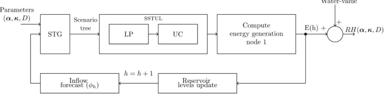
The entire process is composed of five main components and can be viewed on Figure1. The first one is called the scenario tree generator (STG) and it takes as input the scenario tree parameters α and κ, which are respectively the number of child nodes per stage and the aggregation of each stage, as well as the fixed parameter D representing the number of stages of the scenario tree and finally, the daily inflow forecasts denoted φh, where h is the day in the rolling-horizon. As it names indicates, it produces a scenario tree that becomes the input of the second component namely the stochastic short-term unit commitment and loading problem (sstul), which consists of two components. The loading problem (LP) is a nonlinear mixed-integer program that determines the water discharge, reservoir volume and number of active turbines at each node for
sstul Parameters (α, κ, D) Scenario tree LP UC STG Reservoir levels update Inflow forecast (φh) Compute energy generation node 1 h = h + 1 E(h) + + RH(α, κ, D) Water-value
Figure 1: Rolling-horizon scheme. These steps are repeated for each day h of the rolling-horizon.
each power plant. This information is fed to the unit commitment problem (UC), a linear integer program and it determines the exact combination of turbines to use in order to maximize the total energy production at each node and penalize turbines start-up. The output of the sstul is the solution to the sstul optimization problem and is used to compute the energy generation for the first node in the scenario tree, denoted E(h), in which turbine startups are penalized. From here, the reservoir levels are updated with the actual realization of the inflows in the component named reservoir level update. These 5 components are iteratively solved for each time period but only the solution for the first node of the scenario tree is retained every day, allowing to build a release policy for the whole rolling-horizon. The output of the rolling-horizon, namely RH(α, κ, D) is the summation of the energy generation E(h) for each day h of the rolling-horizon, more precisely the first node energy generation every day with startups penalized and the value of the remaining water in the reservoirs at the end of the rolling-horizon.
The objective is to maximize the total energy production over the whole rolling-horizon, by evaluating the energy production for the first stage solution of each day in the rolling-horizon, penalizing turbine startups and considering the value of the remaining water in the reservoirs.
2.3
Parameters of the scenario tree
The overall energy estimated over the rolling-horizon depends on the way that the scenario trees are generated. Generation of these trees depend on a set of three parameters. The main objective of the present work is to tune the values of these parameters so that the overall energy is maximized. The authors formulate this question as a blackbox optimization problem: find the scenario tree parameter values that maximize the energy production. This Section describes in more details the scenario tree parameters.
The scenario tree generating method requires input parameters: number of stages, number of child nodes per stage as well as aggregation of each stage. In addition, it requires as input the inflow scenarios denoted by φ. As the effect of the number of stages is investigated, it is kept as a varying parameter. As for the number of nodes per stage and aggregation, they are treated as blackbox optimization variables. Each node of the scenario trees has at most two child nodes. Since the inflow forecast is for 30 days, it is necessary to aggregate the days into stages in the scenario tree in order to reduce the number of optimization variables. The first stage is not aggregated and hence is not an optimization variable.
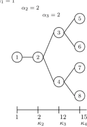
Let D be the number of stages, αq the number of child nodes, for each node q ∈ {1, 2, . . . , D − 1} and κr is the number of days aggregated in stage r ∈ {2, 3, . . . , D}. Figure2illustrates a scenario tree with 4 stages, with α = (1, 2, 2) and κ = (2, 12, 15). With an inflow forecast of 30 days, the following is to be satisfied: P4
The function that characterizes the scenario tree generation is compactly denoted by:
ST G(α, κ, φ), (1)
where α ∈ ND−1
is the number of child node per stage, κ ∈ ND−1 is the aggregation of each stage and φ is the collection of inflow scenarios. The scenario tree generation returns a scenario tree determined by the parameters α and κ, the collection of inflow scenarios φ and a value of inflow for each reservoir and scenario tree node is returned.
1 2 4 8 7 3 6 5 α1= 1 α2= 2 α3= 2 1 2 κ2 12 κ3 15 κ4
Figure 2: A scenario tree with D = 4 stages.
2.4
Loading and unit commitment problems
The loading problem takes as input a scenario tree determined by the parameters α, κ and φ obtained with ST G(α, κ, φ). The loading problem returns the water flows, reservoir volumes and number of turbines working, for every plant and scenario tree node. The loading problem maximizes the energy production in the first stage and expected energy production in the future, subject to water balance constraints and hydropower production functions selection. The entire model is presented in Section 4.2 of (S´eguin et al., 2015).
The function that characterizes the loading problem is compactly denoted by:
LP (ST G(α, κ, φ)). (2)
The loading problem is a nonlinear mixed-integer problem, but the relaxation of binary variables is sufficient (S´eguin et al., 2016) to obtain an integer solution over certain conditions. In this specific case, the energy demand is not considered.
The unit commitment problem takes as input the output of the loading problem, more precisely the water flows, reservoir volumes and number of turbines working, for every plant and scenario tree node. It also requires the scenario tree structure as input, determined with ST G(α, κ, φ). The unit commitment problem consists at maximizing the energy production in the first stage and expected energy production in the future and penalizes startups of turbines, subject to turbine selection and turbine startups constraints. The unit commitment problem returns the turbines working for every plant and scenario tree node. The entire model is presented in Section 4.3 of (S´eguin et al., 2015).
The function that characterizes the unit commmitment problem is complactly denoted by:
U C(LP (ST G(α, κ, φ))). (3)
The unit commitment problem is a linear integer program.
In order to solve the sstul problem in a rolling-horizon framework, it is necessary to solve the loading problem and then the unit commitment problem. Solution for the first day in the scenario tree is kept, then
the reservoir volumes are updated with the actual realization of the inflow that occurred that day. LP and U C require generating the scenario tree before the optimization is conducted.
3
Blackbox optimization
This section introduces the concept of blackbox optimization. Then, the formulation of the rolling-horizon scheme as a blackbox optimization problem is exposed. Finally, the validation of the formulation of the problem as a blackbox is presented.
3.1
Blackbox optimization concept
Blackbox optimization targets problems in which the objective function and/or constraints can only be computed through a computer simulation. Blackbox optimization problems are often nonsmooth, nonconvex and discontinuous. The mesh adaptive direct search method (mads) (Audet and Dennis Jr., 2006) is designed for blackbox optimization and has been successfully applied to many engineering problems.
mads discretizes the state space by defining a mesh whose coarsness is adjusted at the end of each iteration. The algorithm consists of two steps that are repeated until a predefined stopping criteria is reached. The first step, namely the search step evaluates different points that lie on this mesh with the aim of finding a better solution than the current best. This step is flexible and may be taylored to specificities of the problem. The second step, namely the poll step is mandatory as the convergence properties of mad relies on it. A positive spanning set of directions is determined and if a better solution than current best is found, it is set as best solution. During the different iterations, the mesh size is reduced when the algorithm fails to improve the solution and increased when a new best solution is found. The nomad software (Le Digabel, 2011), which is the implementation of the mads method is used to solve the blackbox optimization model.
3.2
Blackbox formulation of the rolling-horizon scheme
The scenario tree parameters α and κ that maximizes the energy production throughout the rolling-horizon are to be identified. A blackbox that takes a tree structure as input, and solves the whole rolling-horizon scheme, which contains the scenario tree generation and the sstul optimization problem is defined. It returns the total energy produced throughout the rolling-horizon.
3.2.1 Mathematical formulation
The scenario tree parameters α and κ are the optimization variables provided as input to the blackbox. The output of the blackbox is the total energy produced, considering startup penalties and value of remaining water in the reservoir in the rolling-horizon scheme. The sstul optimization variables, which are water discharge, reservoir volumes and turbines working are internal to the blackbox and are transparent to the blackbox optimization problem.
Therefore, the blackbox optimization problem is to maximize total energy produced throughout the rolling-horizon scheme, with startups penalized and value of the water remaining in the reservoirs. The output of the blackbox is compactly denoted by:
RH(α, κ, D), (4)
where D is fixed and is the number of stages in the scenario tree.
The objective function given by Equation(5) is to maximize energy production throughout the rolling-horizon, considering startup penalties and value of remaining water in the reservoirs. It relates to the unit commitment problem and since this solution relies on the output of the loading problem, problems UC and LP are to be solved in order to obtain the value of RH(α, κ, D). In other words, it is necessary to solve the sstul problem when solving the blackbox optimization problem.
Problem BB : max α,κ ∈ ND−1 RH(α, κ, D) (5) subject to: D X r=2 κr= 29, (6) 2 ≤ D−1 Y q=1 αq≤ 50, (7) αq, κr> 1 , ∀q ∈ {1, 2, . . . , D − 1} , ∀r{∈ 2, 3, . . . , D}. (8)
The main difficulty of the problem above resides in evaluating RH(α, κ, D). Computational time required to evaluate the blackbox increases with the complexity of the scenario trees, rather than with the number of optimization variables. For example, for a 5 stage scenario tree and α = (1, 4, 3, 3), a total of 52 nodes, a single evaluation of RH(α, κ, D) takes 32 minutes, on a given data set, while a 6 stage scenario tree and α = (2, 5, 5, 1, 1), a total of 162 nodes, takes 1 hour. Moreover, there is only a difference of 2 optimization variables between these scenario tree structures.
Constraints (6) are to ensure the aggregation of the scenario tree stages are equivalent to the inflow forecast, which is 30 days in this paper. Since the first stage is not aggregated then it is forced to 1. The upper and lower bounds on the number of scenarios are given by (7). Nonnegativity is enforced with constraints (8). The number of stages D is kept as a varying parameter in the numerical experiments in order to evaluate its effect on the results. Hence, it is fixed for every experiment.
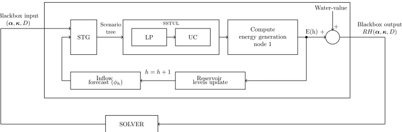
Figure 3 illustrates this process. A scenario tree structure with parameters α and κ is given to the blackbox. The rolling-horizon scheme is then launched. For every day of the rolling-horizon, scenario trees are built based on the forecast φh, then the sstul is solved, the first day solution is kept, reservoir levels are updated with the realization of inflows and the process is repeated for the whole rolling-horizon. Then, the actual energy production and expected future production of the remaining water in the reservoir for the whole rolling-horizon is calculated, with startups of turbines penalized and is denoted RH(α, κ, D). The optimization solver calls the blackbox simulation with various values of the parameters α and κ. Each time the solver collects the output RH(α, κ, D) and from it, it produces new inputs to the blackbox. The solver terminates when it can no longer improve the solution.
sstul Blackbox input (α, κ, D) Scenario tree LP UC STG Reservoir levels update Inflow forecast (φh) Compute energy generation node 1 h = h + 1 E(h) + Blackbox output RH(α, κ, D) + Water-value SOLVER
Figure 3: The blackbox optimization problem. Index h is the day in the rolling-horizon framework.
3.3
Blackbox validation
The scenario tree generation method applied in this paper is stochastic, which means that for the same set of scenario tree parameters, the inflow values on the nodes of the scenario tree differ from one evaluation to the other. Therefore, the objective function value RH(α, κ, D) of the blackbox differs for the same structure of scenario trees. The blackbox is validated to ensure that trying to optimize the scenario tree parameters
is relevant. Since the scenario tree generation method is stochastic, the state space changes dynamically while the solver is searching for scenario tree parameters values. Therefore, it is important to assess that the variation of the state space is negligible compared to converging towards a solution. A fixed scenario tree structure is used and the blackbox is evaluated 100 times with the same set of scenario tree parameters, on a given data set.
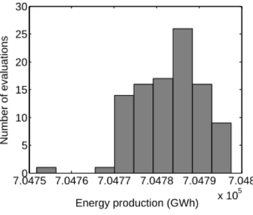
Results of this validation are shown on Figure4. The number of evaluations of the blackbox corresponding to a given range of objective function values are represented on a histogram. The following values were used for the parameters: D = 5, α = (1, 1, 2, 1) and κ = (3, 6, 8, 12). One can see that energy production is very similar at every evaluation of the blackbox, the standard deviation is 7.4622 GW h, compared to a 7.0478 ×10⁵ GW h mean. The values near the mean confirm that the scenario tree generation method is valid, as evaluations of the blackbox with the same scenario tree parameters lead to similar values every time.
7.0475 7.0476 7.0477 7.0478 7.0479 7.048 x 10⁵ 0 5 10 15 20 25 30 Energy production (GWh) Number of evaluations
Figure 4: Validation of the blackbox. For the same scenario tree structure, histogram of the energy production in GW h.
3.3.1 Exhaustive enumeration versus blackbox optimization
To assess the pertinence of using a blackbox optimization problem to find the scenario tree structure that maximizes the energy production in the rolling-horizon, a comparison between the solution found with the blackbox optimization and the global optimal solution is performed.
A 5 stage scenario tree with fixed aggregation of stages κ = (3, 6, 8, 12) is chosen since the state space is relatively small. The problem contains only integer optimization variables, therefore it is possible to do an exhaustive enumeration of the domain. Considering constraints on minimal and maximal number of scenarios, there is a total of 331 points in the state space. Total computational time to run the evaluations cumulates to 27 hours. The best solution found is a tree with a structure α = (5, 1, 2, 3) and the value of the objective is 804.63 T W h. Since the objective function is evaluated at every possible combination of α in the domain, this is the global optimal solution.
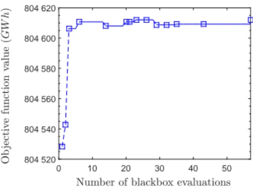
The blackbox optimization solver nomad is used to find the scenario tree that maximizes the energy production throughout the rolling-horizon. The convergence is shown in Figure5. The optimization requires 57 evaluations, but the best solution is found after 23 evaluations. The time to conduct the optimization is 7 hours. The solution found by nomad is a tree with structure α = (4, 5, 1, 2) and the objective is 804.63T W h, which is identical up to the second decimal to that found by the exhaustive enumeration procedure. The Figures shows clearly that in less than 10 evaluations the objective function is substantially decreased.
For this 5 stage scenario tree case, the computational time required by nomad is approximately one fourth of that of the enumeration strategy. The difference between the objective values obtained with the optimization and enumerating all the state space is negligible. Therefore, optimizing the tree structure with nomad allows to find an acceptable solution. Since the scenario tree generation method is stochastic, the objective function value varies for the same scenario tree structure, so it is difficult to assess if nomad found
Number of blackbox evaluations 0 10 20 30 40 50 O b je ct iv e fu n ct io n va lu e (G W h ) 804 620 804 600 804 580 804 560 804 540 804 520
Figure 5: Convergence of blackbox optimization for a 5 stage scenario tree.
the global solution or not, but there is a great decrease in the objective function when the structure of the tree is optimized, as shown in Figure5.
The starting point led to an objective function of 804.46 T W h while the best solution found is 804.63 T W h. The difference between these two values is 0.17 T W h, which is much greater than the standard deviation of 7.4 GW h and confirms that the minimum found by nomad truly is a minimum and not induced by noise.
4
Case study
This sections presents the case study used to validate the optimization models presented in this research.
4.1
Hydropower system
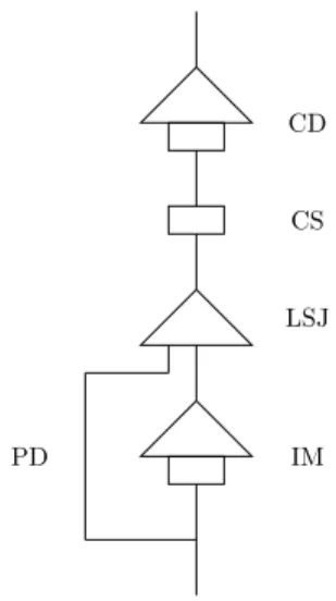
The optimization method presented in this paper is tested on a portion of a hydroelectric system that belongs to Rio Tinto and is shown on Figure6. It is located in Saguenay in the province of Qu´ebec, Canada. The sub-system consists of 4 reservoirs and 3 power plants in series, namely Chute-du-Diable (cd), Chute-Savane (cs), Lac-St-Jean (lsj) and Isle-Maligne (im). Travel time of the water between plants is neglected. The installed capacity for these 3 power plants is about 950 M W . The power plants and reservoirs characteristics are shown in Table1.
Table 1: Reservoir and power plants characteristics. Reservoir and/or Nb. Reservoir capacity power plant turbines (hm3)
CD 5 452
CS 5 119
LSJ - 5596
IM 12 171
4.2
Structure of the data
Six data series are available for numerical experiments. There are 31 days in the rolling-horizon scheme and every day has a 30 day inflow forecast. Figure 7 shows an example of scenario trees for the first day of the rolling-horizon. The scenario trees, in black, are built from the inflow scenarios, which are shown in grey.
5
Computational experiments
Two types of tests for the optimization of the scenario trees are conducted on the data series available. First, the aggregation of the stages is fixed arbitrarily and only the structure of the scenario tree is optimized, for
CD
CS
LSJ
IM PD
Figure 6: Hydroelectric system studied. Squares represent power plants and triangles reservoirs.
Stages 1 2 3 4 5 6 Inflow (\%) 17 34 51 68 85 100 (a) CD Stages 1 2 3 4 5 6 Inflow (\%) 0 17 34 51 68 85 100 (b) CS Stages 1 2 3 4 5 6 Inflow (\%) 0 17 34 51 68 85 100 (c) LSJ Figure 7: Scenario trees built from inflow forecast scenarios.
different values of stages. Therefore, the blackbox optimization variables κ are fixed in the mathematical model BB. For a 5 stage scenario tree, there are 4 blackbox optimization variables α, which are the structure of stages 2, 3, 4 and 5. For a 9 stage scenario tree, there are 8 blackbox optimization variables. Second, the structure and the aggregation of the stages is optimized, for different values of stages. For a 9 stage scenario tree, there are 16 blackbox optimization variables, more precisely α are the structure and κ the aggregation of each stage.
The solver ipopt (W¨achter and Biegler, 2006) is used for the loading problem, xpress (, Xpr) for the unit commitment problem and nomad (Le Digabel, 2011) for the blackbox optimization problem.
5.1
Deterministic optimization with the median scenario
In this section, results of the sstul with optimized scenario tree parameters are compared to a deterministic optimization where only the median scenario in the forecast is used. First, results with optimization of the structure only and a fixed aggregation and second, results with optimization of the structure and aggregation. Optimizing the sstul with a median scenario comes down to solving a deterministic model. For the producer, comparing the solution obtained from the stochastic model gives a value on the interest of investing time to solve a stochastic model.
Basically, the same rolling-horizon scheme for the stochastic method and the deterministic optimization is used. For the stochastic method, a scenario trees based on the inflow forecast is generated and the sstul model is solved. For the median scenario method, the median scenario out of all of the inflow scenarios is chosen and a deterministic model is solved.
5.1.1 Optimization of the structure only
The solution obtained with the sstul model and optimization of the structure of the scenario tree is compared to the solution obtained when solving the sstul with the median scenario.
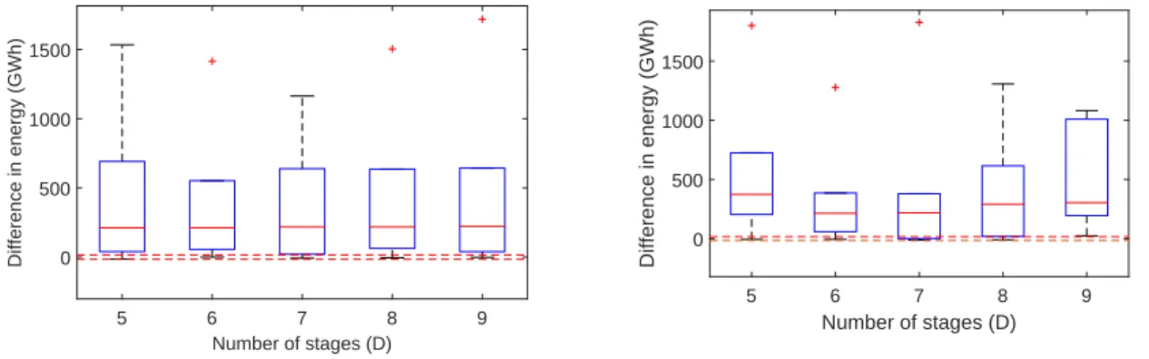
Results are presented with a boxplot for every number of stages and all 6 test cases, as seen on Figure8a. For stages ranging from 5 to 9, the boxplot of the difference in energy between the stochastic solution, for which the scenario trees structure is determined with blackbox optimization, and the median scenario is shown. A positive value indicates the stochastic method produces more energy. As explained previously, since the scenario tree generation method is stochastic, two standard deviations are required for the difference in energy to be valid and not blackbox noise, more precisely ±16 GW h and are shown on Figure8awith the pair of horizontal dotted-lines.
Figure 8a illustrates that, with an arbitrarily aggregation of the stages, optimizing the structure of the scenario tree leads to similar results for ever given number of stages. Therefore, the number of stages does not have an important influence on the energy production in the sstul problem.
5.1.2 Optimization of the structure and the aggregation
The solution obtained with the sstul model and optimization of the structure and the aggregation of the scenario tree is compared to the solution obtained when solving the sstul with the median scenario.
Figure 8b illustrates the results for the 6 test cases. For a number of stages varying from 5 to 9, the difference in energy between the stochastic solution and the deterministic optimization, a boxplot is displayed. When the value is positive, it signifies that the stochastic method produced more energy. The pair of horizontal dotted-lined at ±16GW h represent the two standard deviations that ensure the difference in energy is not noise induced by the blackbox.
Figure 8b reveals that optimizing the scenario tree structure and aggregation increases the difference between the stochastic solution and median scenario given a higher number of stages. Therefore, the aggre-gation of the stages is an important parameter in the scenario tree generation method, as the difference in energy increases when the number of stages increases.
5.2
Scenario fans
Relying on the median scenario to implement a decision is highly risky. Often, in hydropower optimization, scenario fans are used in the optimization models since they present a compromise between investing a lot of time and effort in generating the trees and solving a stochastic multi-stage model and solving a deterministic model. This Section presents, for different number of stages, comparisons with different numbers of scenarios
Number of stages (D) 5 6 7 8 9 Difference in energy (GWh) 0 500 1000 1500
(a) Optimization of the structure of the scenario tree only.
Number of stages (D) 5 6 7 8 9 Difference in energy (GWh) 0 500 1000 1500
(b) Optimization of the structure and aggregation of the scenario tree.
in a scenario fan fashion, as shown in Figure9. The same scenario tree generation method than used previously was used to generate the trees, given different values of stages and number of scenarios. For the aggregation, the value obtained during the blackbox optimization of the scenario tree structure and aggregation was used, as it is the one that maximizes energy production. For example, a structure α = (1, 25, 1, 1) is given as input to the STG to obtain a scenario fan of 25 scenarios and 5 stages.
Scenario 1
Scenario . . .
Scenario x
Stage Stage Stage . . . Stage Stage 1 2 3 . . . D-1 D
Figure 9: Scenario fan with x scenarios and D stages.
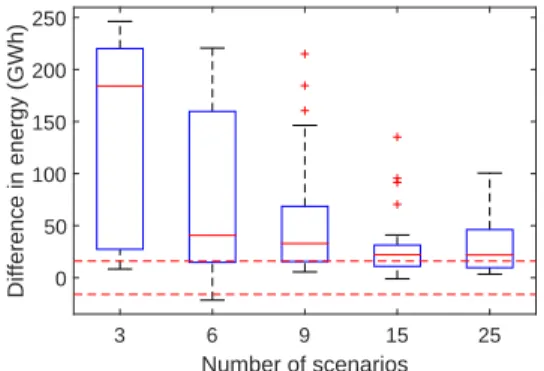
Multiple tests were conducted on the different test cases. For 5, 6, 7, 8 and 9 stages, scenarios fans of 3, 6, 9, 15 and 25 scenarios were used as input to the sstul model. As explained previously, since the scenario tree generation method is stochastic, two standard deviations are required for the difference in energy to be valid and not blackbox noise, more precisely ±16 GW h and are shown on Figure 10 with the pair of horizontal dotted-lines. Results are presented in Figure10. The difference in energy between the stochastic optimization and scenario fans decreases when the number of scenarios increase. Therefore, solving the sstul with a scenario fan containing more than 15 scenarios results in the same objective function and does not justify the use of a complex scenario tree structure. Standard deviation for 15 scenarios is 30.6973 GW h and for 25 scenarios is 26.4338 GW h. Moreover, a Student’s t-test performed on the distributions of 15 and 25 scenarios reject the null hypothesis, therefore demonstrating that the difference in energy is significant and not caused by blackbox noise.
These results demonstrate that using scenario fans instead of complex scenario tree structures leads to good results and allows to find the solution in a satisfying computational time effort. Also, the scenario fan results show that the distribution of the total volume of inflows is preserved if the scenario tree generation method does not alter the scenarios, therefore by using, in this case, more than 15 scenarios. Moreover, in a rolling-horizon, the decision that is taken at the first node every day is mostly influenced by the total volume of water to be received, rather than by the structure of the scenario trees that model the distribution of the inflows. Number of scenarios 3 6 9 15 25 Difference in energy (GWh) 0 50 100 150 200 250
Figure 10: Boxplots of the difference in energy production between stochastic optimization of the structure and the aggregation of the scenario tree compared to scenario fans.
It is important to note that when using scenario fans, only the first node solution is relevant since the rest of the stages is biased, induced by the deterministic fashion of the scenario fan. When using scenario trees, non-anticipative constraints appear at each stage, therefore all of the inflow values contained in the scenario tree are relevant and could be useful in another context.
6
Conclusion
In this paper, the authors have presented an innovative method to determine if complex scenario tree struc-tures are required when solving the short-term unit commitment and loading problem (sstul) with uncertain inflows used in an real-time decision making context. Multistage stochastic programs are used to solve the sstul problem and the modeling of the problem allows to account for head-dependency as well as limit turbine restarts. In an operational context, a rolling-horizon scheme is used to implement the solutions. Every day, forecasts of inflows are available. From these, a scenario tree is constructed to represent the distribution of the inflows, then the optimization models are solved. The solution is implemented and the reservoir volumes are updated once the real realization of the inflows are known. Only the solution for the first node every day is retained, as new forecasts become available and that the process is repeated. The scenario tree generation method that is used requires input parameters, which are the number of sates, child node per stage as well as the aggregation of each stage.
To measure the benefits of using complex scenario tree structures, the whole rolling-horizon was modeled as a blackbox optimization model, to find the scenario tree parameters that maximize the energy production throughout the rolling-horizon, for different values of the number of stages. Results are compared with scenario fans and they show that the decision taken at the first node every day is mostly influenced by the volume of inflows, rather than the structure of the scenario trees, which means that using scenario fans leads to good results and requires less computational time.
7
Notation
The following symbols are used in this paper: D = number of stages ;
E(h) = energy produced per day h with startups penalized ; h = index of the rolling-horizon h = (1, 2, . . . , 31) (days) ; LP (ST G(α, κ, φ)) = loading problem function;
q = index of the number of child nodes per stage r = (1, 2, . . . , D − 1) ; r = index of the aggregation per stage r = (2, 3, . . . , D) ;
RH(α, κ, D) = blackbox function ;
ST G(α, κ, φ) = scenario tree generation function; U C(LP (ST G(α, κ, φ))) = unit commitment function.
αq = number of child nodes per stage q ; κr = aggregation of each stage r (days); and
References
XPRESS Optimization Suite, Fair Isaac Corporation (FICO). www.fico.com/en/products/fico-xpress-optimization-suite/.
Alarie, S., Audet, C., Garnier, V., Le Digabel, S., and Leclaire, L.-A. (2013). Snow water equivalent estimation using blackbox optimization. Pacific Journal of Optimization, 9(1), 1–21.
Audet, C. (2014). A survey on direct search methods for blackbox optimization and their applications. Mathematics Without Boundaries: Surveys in Interdisciplinary Research, M. P. Pardalos and M. T. Rassias, eds., Springer, New York, 31–56.
Audet, C., Dang, K.-C., and Orban, D. (2014). Optimization of algorithms with opal. Mathematical Programming Computation, 6(3), 233–254.
Audet, C. and Dennis Jr., J. E. (2006). Mesh adaptive direct search algorithms for constrained optimization. SIAM Journal on Optimization, 17(1), 188–217.
Belsnes, M., Wolfgang, O., Follestad, T., and Aasg˚ard, E. (2016). Applying successive linear programming for
stochastic short-term hydropower optimization. Electric Power Systems Research, 130, 167–180.
Beraldi, P., Violi, A., Scordino, N., and Sorrentino, N. (2011). Short-term electricity procurement: A rolling horizon stochastic programming approach. Applied Mathematical Modelling, 35(8), 3980–3990.
Cˆot´e, P. and Leconte, R. (2016). Comparison of stochastic optimization algorithms for hydropower reservoir operation with ensemble streamflow prediction. Journal of Water Resources Planning and Management, 142(2).
Follestad, T., Wolfgang, O., and Belsnes, M. M. (2011). An approach for assessing the effect of scenario tree approx-imations in stochastic hydropower scheduling models. Proc. of the 17th Power System Computation Conference, 271–277.
Heitsch, H. and R¨omisch, W. (2009). Scenario tree reduction for multistage stochastic programs. Computational
Management Science, 6(2), 117–133.
Høyland, K., Kaut, M., and Wallace, S. (2003). A heuristic for moment-matching scenario generation. Computational Optimization and Applications, 24(2), 169–185.
Kaut, M. (2014). A copula-based heuristic for scenario generation. Computational Management Science, 11(4),
503–516.
Le Digabel, S. (2011). Algorithm 909: NOMAD: Nonlinear optimization with the MADS algorithm. ACM Transac-tions on Mathematical Software, 37(4), 44:1–44:15.
Minville, M., Cartier, D., Guay, C., Leclaire, L.-A., Audet, C., Le Digabel, S., and Merleau, J. (2014). Improving process representation in conceptual hydrological model calibration using climate simulations. Water Resources Research, 50(6), 5044–5073.
Moazeni, S., Defourny, B., and Hajimiragha, A. H. (2015). Risk-sensitive stochastic optimization for storage operation management. Smart Energy Grid Engineering (SEGE), 2015 IEEE International Conference on, 1–6 (Aug).
Morin, G. and Paquet, P. (2007). Mod`ele hydrologique cequeau. Report No. R926, INRS, Centre Eau, Terre et
Environnement.
Pflug, G. Ch. and Pichler, A. (2015). Dynamic generation of scenario trees. Computational Optimization and
Applications, 1–28.
Santo, T. D. and Costa, A. S. (2016). Hydroelectric unit commitment for power plants composed of distinct groups of generating units. Electric Power Systems Research, 137, 16–25.
Scott, D. W. (2015). Multivariate density estimation: theory, practice, and visualization. John Wiley & Sons. S´eguin, S., Cˆot´e, P., and Audet, C. (2016). Self-scheduling short-term unit commitment and loading problem. IEEE
Transactions on Power Systems, 31(1), 133–142.
S´eguin, S., Fleten, S.-E., Pichler, A., Cˆot´e, P., and Audet, C. (2015). Stochastic short-term hydropower planning with inflow scenario trees. Cahier du gerad, (G-2015-97) Revised June 2016.
W¨achter, A. and Biegler, L. (2006). On the implementation of an interior-point filter line-search algorithm for large-scale nonlinear programming. Mathematical Programming, 106(1), 25–57.
Xu, B., Zhong, P.-A., Zambon, R. C., Zhao, Y., and Yeh, W. W.-G. (2015). Scenario tree reduction in stochastic programming with recourse for hydropower operations. Water Resources Research, 51(8), 6359–6380.
Zhao, T., Yang, D., Cai, X., Zhao, J., and Wang, H. (2012). Identifying effective forecast horizon for real-time reservoir operation under a limited inflow forecast. Water Resources Research, 48(1).