Modeling commodity prices for
valuation and hedging of mining
projects subjected to volatile markets
Mathieu Sauvageau
Doctor of Philosophy
Mining and Materials Engineering
McGill University Montreal,Quebec
July 2017
A thesis submitted to McGill University in partial fulfillment of the requirements of the degree of Doctor of Philosophy
c
ACKNOWLEDGEMENTS
I would like to express my gratitude to my supervisor Dr. Mustafa Kum-ral for giving me the opportunity to perform research in a field which I am passionate about, finance. I hope my contribution will help the Mineral eco-nomics, mine reliability and asset management lab to gain a greater exposure in the research community.
I would also like to thank my lab colleagues Salvatore, Martha, Asli, Tarek, Burak, Aldin and Faruk for sharing your thoughts on my research, but more importantly, your extremely rich and diversified backgrounds. A special men-tion goes to Salvatore for cooking me pasta and showing me how to make my own pizza Margherita.
I would also like to thank my life partner, Joanie, for accepting to put all kinds of projects on hold while I am still a student. Believe me, I will prove to you that it was well worth the wait! I would also like to thank my parents for encouraging me to pursue my studies. My mother always said when you like what you are doing you will never have to work. I pretty much apply this concept on an every day basis and I can’t stress enough how much it is true. My father has always been there for me, giving me advice when needed. I am glad to have a very supportive family which values education and hard work.
CONTRIBUTION OF AUTHORS
The author of this thesis is the primary author for all manuscripts con-tained within. Professor Mustafa Kumral is the supervisor of the candidate Ph.D., and is included as a second author for each of these manuscripts. Chapter 3 - Sauvageau, Mathieu, and Mustafa Kumral. “Analysis of Min-ing EngineerMin-ing Data UsMin-ing Robust Estimators in the Presence of Outliers.” Natural Resources Research 24.3 (2015): 305-316.
Chapter 4 - Sauvageau, Mathieu, and Mustafa Kumral. (under review) “A Kalman filtering approach to model Net Present Value of an iron mine.” Nat-ural Resources Research.
Chapter 5 - Sauvageau, Mathieu, and Mustafa Kumral. “Genetic algorithms for the optimization of the Schwartz-Smith two-factor model: A case study on a copper deposit.” International Journal of Mining, Reclamation and En-vironment. http://dx.doi.org/10.1080/17480930.2016.1260858
Chapter 6 - Sauvageau, Mathieu, and Mustafa Kumral. Under revision “Cash-Flow at Risk valuation of mining project using Monte-Carlo simula-tions calibrated on historical data”, The Engineering Economist.
ABSTRACT
Duration between discovery of a mineral deposit and delivery of the ma-terial (e.g. metal or concentrate) yielded from this deposit to the market can take several years. After the discovery, a feasibility study is conduced to see if the mining operation on this deposit is economically viable. This feasibility study is exposed to two types of uncertainties, which add to risks to the mining project. These are (1) technical risks arising from sparse data (e.g. grade, re-covery and geotechnical characterization) and (2) financial risks arising from unknown future events (e.g. commodity price, discount rate and exchange rate). Among the others, commodity price is a significant concern for the executives of mining enterprise. Given that mining products and their deriva-tives are traded in commodity, stock and future markets, market dynamics are very complex. Furthermore, it is very sensitive to politics of global world and very open to speculation and manipulation as well as demand and supply. In the past, the mining industry witnessed that many mining operations were suspended or ceased due to unresponsiveness to price fluctuations. Project val-uation based on log-term price is a quite naive approach at present day. This can jeopardize the financial resources of the investor company. Therefore, the risks associated with commodity price are assessed, quantified, mitigated, di-versified or managed. The analysis of commodity prices starts with the study of historical transactions in financial markets. To facilitate the analysis, it is often necessary to convert commodity prices into returns. Then, the next task is to model the distribution of returns using a statistical distribution. One of the main characteristics of the distribution of commodity price returns is that it tends to have excess kurtosis. This can be explained either by a
the evolution of prices. For this reason, it is necessary to consider other models than the Geometric Brownian Motion and Mean-Reverting price models when modeling the dynamics of commodity prices. The objective of this thesis is to construct a robust workflow capable of reproducing the observed price dy-namics in the commodity markets. With such calibrated models, it is possible to value mining projects or estimate their exposure to market risk. In the first case, the valuation process is made in a risk-neutral framework using a Real Options approach. In the second case, real world probabilities are used to simulate commodity price paths and assess how a mining project may be exposed to market price fluctuations. Following an introduction and a Liter-ature review, the thesis is divided in four additional parts, corresponding to four different publications. In the first publication, the use of robust estimators for the detection and mitigation of outliers is investigated. The paper starts with an overview of multiple linear regression and assess how the model as-sumptions can be violated. The second part of the paper deals with detecting outliers using studentized residuals or the Mahalanobis distance. Then robust regression is used to diminish the effects of outliers in mining engineering data including price. The second paper investigates how the dynamics of iron ore future can be modeled with a dynamic linear model. Traditionally, iron ore futures have been traded using long-term commitment contracts. This paper investigates how relatively recent financial instruments such as futures on iron ore can affect the NPV profile of an iron ore project. The third paper deals with the optimization of the parameters in a commodity model using a genetic algorithm. With correctly calibrated parameters, Monte Carlo simulations of commodity spot and futures are performed and an active trading strategy is implemented in an NPV valuation framework. The last publication deals with
the choice of the stochastic process when measuring market risk of a min-ing project. Several stochastic processes are calibrated on historical data and used to calculate the cash flow at risk of a mining project. The models are calibrated using an hybrid metaheuristic calibration strategy. Particle swarm optimization is first used to find a solution close to the global minimum. Then, a gradient based routine is used to find the optimal solution.
ABR´EG´E
Plusieurs ann´ees se produisent habituellement entre la d´ecouverte d’un nouveau gisement min´eral et la livraison des mat´eriaux produits sur les march´es financiers. Une ´etude de faisabilit´e est g´en´eralement effectu´ee pour ´evaluer la viabilit´e du projet minier. L’une des tˆaches les plus importantes est d’´evaluer la valeur actuelle nette du projet minier. Cette variable est la somme des flux de tr´esorerie actualis´es que le projet minier g´en´erera au cours de sa dur´ee de vie. Les flux de tr´esorerie sont actualis´es `a un niveau appropri´e pour refl´eter le risque du projet. Quantifier le risque des projets miniers peut ˆetre une tˆache encombrante. En effet, les projets miniers sont soumis `a de multiples sources d’incertitudes qui doivent ˆetre estim´ees `a l’aide de mod`eles stochastiques. L’une de ces inconnues est le prix des produits de base, qui doit ˆetre pro-jet´e sur toute la dur´ee du projet minier. Pour faciliter l’analyse, il est souvent n´ecessaire de convertir les prix des mati`eres premi`eres en rendements. Ensuite, la tˆache suivante consiste `a mod´eliser la distribution des rendements `a l’aide d’une distribution statistique. L’une des principales caract´eristiques de la dis-tribution des rendements des prix des produits de base est qu’il tend `a avoir un exc`es de kurtosis. Cela peut ˆetre expliqu´e soit par une volatilit´e stochastique ou une composante de saut dans l’´equation de diffusion d´ecrivant l’´evolution des prix. Pour cette raison, il est n´ecessaire d’envisager d’autres mod`eles que les mod`eles de mouvement g´eom´etrique brownien et de r´eversion moyenne lors de la mod´elisation de la dynamique des prix des produits de base. L’objectif de cette th`ese est de construire un workflow robuste capable de reproduire la dynamique des prix observ´ee sur les march´es des mati`eres premi`eres. Avec ces mod`eles calibr´es, il est possible d’´evaluer les projets miniers ou d’estimer leur exposition au risque de march´e. Dans le premier cas, le processus d’´evaluation
est effectu´e dans un cadre risque-neutre en utilisant une approche ax´ee sur les options r´eelles. Dans le second cas, les probabilit´es r´eelles sont utilis´ees pour simuler les sc´enarios de prix des produits de base et pour ´evaluer com-ment un projet minier peut ˆetre expos´e aux fluctuations des prix du march´e. La th`ese est divis´ee en quatre parties, correspondant `a quatre publications diff´erentes. Dans la premi`ere publication, l’utilisation d’estimateurs robustes pour la d´etection et l’att´enuation des valeurs aberrantes est ´etudi´ee. L’article commence par un aper¸cu de la r´egression lin´eaire multiple et ´evalue comment les hypoth`eses du mod`ele peuvent ˆetre viol´ees. La deuxi`eme partie de l’article traite de la d´etection des valeurs aberrantes en utilisant des r´esidus studenis´es ou la distance de Mahalanobis. Puis, une r´egression robuste est utilis´ee pour diminuer les effets des valeurs aberrantes dans les donn´ees d’ing´enierie mini`ere. Le second article ´etudie comment la dynamique du minerai de fer peut ˆetre mod´elis´ee avec un mod`ele lin´eaire dynamique. Traditionnellement, les contrats `
a terme de minerai de fer ont ´et´e n´egoci´es `a l’aide de contrats d’engagement `
a long-terme. Cet article ´etudie comment des instruments financiers relative-ment r´ecents comme les contrats `a terme sur le minerai de fer peuvent affecter le profil de la VAN d’un projet de minerai de fer. Le troisi`eme article traite de l ’optimisation des param`etres dans un mod`ele de marchandise utilisant l’ algorithme g´en´etique. Avec des param`etres correctement ´etalonn´es, des sim-ulations Monte Carlo de spot et de contrats `a terme sur mati`eres premi`eres sont effectu´ees et une strat´egie de n´egociation active est mise en œuvre dans un cadre d’´evaluation VAN. La derni`ere publication traite du choix du pro-cessus stochastique lors de la mesure du risque de march´e d’un projet minier. Plusieurs processus stochastiques sont ´etalonn´es sur des donn´ees historiques et utilis´es pour calculer le flux de tr´esorerie `a risque d’un projet minier. Les mod`eles sont calibr´es en utilisant une strat´egie de calibration m´etaheuristique
hybride. L’optimisation des essaims de particules est d’abord utilis´ee pour trouver une solution proche du minimum global. Ensuite, une routine bas´ee sur le gradient est utilis´ee pour trouver la solution optimale.
TABLE OF CONTENTS
ACKNOWLEDGEMENTS . . . ii
CONTRIBUTION OF AUTHORS . . . iii
ABSTRACT . . . iv
ABR´EG´E . . . vii
LIST OF TABLES . . . xiii
LIST OF FIGURES . . . xv 1 Introduction . . . 1 1.1 Overview . . . 1 1.2 Original Contributions . . . 4 2 Literature Review . . . 7 2.1 Overview . . . 7
2.2 Market risk regarding commodity markets . . . 9
2.3 Robust regression . . . 12
2.4 Stochastic processes . . . 14
2.5 State space representation of stochastic processes . . . 18
2.6 Genetic algorithms . . . 21
2.7 Options pricing theory in financial markets . . . 23
2.8 Introduction to Real Options valuation . . . 25
3 Analysis of mining engineering data using robust estimators in the presence of outliers . . . 29
3.1 Abstract . . . 29
3.2 Introduction . . . 30
3.3 Outliers detection . . . 34
3.4 Robust regression . . . 35
3.4.1 The least absolute regression model (L1 estimator) . 37 3.4.2 M-estimator . . . 38
3.4.3 LTS estimator . . . 39
3.4.4 LMS estimator . . . 39
3.4.5 MM-estimator . . . 40
3.5.1 Mineral processing costs recovery relation . . . 41
3.5.2 Iron and alumina grade relation . . . 45
3.6 Conclusion . . . 48
3.7 Chapter Conclusion . . . 49
4 A Kalman filtering approach to model net present value of an iron mine . . . 50
4.1 Abstract . . . 50
4.2 Introduction . . . 51
4.3 Methodology . . . 56
4.3.1 Model Input Data . . . 56
4.3.2 Maximum Likelihood Optimization . . . 61
4.3.3 Schwartz Two-Factor Model . . . 62
4.4 Results . . . 65
4.4.1 Time Series Analysis . . . 65
4.4.2 Kalman Filtering . . . 69
4.5 Conclusion . . . 78
4.6 Appendix . . . 80
4.7 Chapter Conclusion . . . 81
5 Genetic algorithms for the optimization of the Schwartz-Smith two-factor model: A case study on a copper deposit . . . 82
5.1 Abstract . . . 82
5.2 Introduction . . . 83
5.3 Methodology . . . 88
5.3.1 Schwartz-Smith two-factor model . . . 88
5.3.2 Genetic algorithms . . . 92
5.3.3 NPV Incorporating an active trading strategy . . . 94
5.4 Case study . . . 96
5.4.1 Data . . . 96
5.4.2 Two-factor model calibrated on artificial data . . . . 101
5.4.3 Two-factor model calibrated on crude oil futures prices103 5.4.4 Two-factor model calibrated on copper prices . . . . 106
5.4.5 NPV valuation of a copper mine . . . 109
5.5 Discussion . . . 112
5.6 Conclusion . . . 115
5.7 Chapter Conclusion . . . 117
6 Cash-flow at risk valuation of mining project using Monte-Carlo simulations calibrated on historical data . . . 118
6.1 Abstract . . . 118
6.2 Introduction . . . 118
6.3 Literature review . . . 120
6.4.1 Merton jump-diffusion models . . . 123
6.4.2 Stochastic volatility models . . . 124
6.4.3 Estimation of CFaR . . . 127 6.5 Case study . . . 128 6.5.1 Data . . . 128 6.5.2 Model calibration . . . 134 6.5.3 CFaR analysis . . . 137 6.6 Discussion . . . 139 6.7 Conclusion . . . 141 7 Conclusion . . . 145
LIST OF TABLES
Table page
3–1 Summary of the OLS Performed on the Original Processing Costs and Recovery Dataset as Well as on the Cleaned
Dataset Where Observation 14 was Dropped. . . 43 3–3 Summary of OLS-, L1-, M-, LTS-, LMS-, and MM-Estimation
Intercept and Coefficient . . . 45 3–5 Summary of OLS-, L1-, M-, LTS-, LMS-, and MM-Estimation
Intercept and Coefficient . . . 47 4–1 Summary statistics for the training and prediction sets of the
iron ore time series. . . 65 4–2 Initial and optimized parameters with the MLE algorithm after
300 iterations . . . 69 5–1 Parameters used in simulations of the SSTF model. These
parameters are taken from the original publication of Schwartz and Smith (2000a). . . 97 5–2 Minimum, maximum and the simulated values of the parameters
in the SSTF model simulations. Simulated values are the parameters the GA will try to retrieve and the range between minimum and maximum value is the search space for the
optimal solution. . . 101 5–3 Optimal parameters after 25 generations of the GA for different
period lengths T. . . 103 5–4 Optimal solution of the GA after 25 generations . . . 104 5–5 Mean error, standard deviation of errors and mean absolute
deviation of the fitted maturities for the crude oil futures
dataset. . . 106 5–6 Parameters of the original Goodwin (2013) paper and
param-eters optimized with the GA for two different sub-periods
affected by different market dynamics. . . 107 5–7 Mean error, standard deviation of errors and mean absolute
5–8 cash flows of the mining project. The project lasts 12 years with an initial outlay of $175 millions. Mining costs are the costs to extract the materials from the mine and processing costs are the costs to extract the metal from the ore. . . 110 6–1 Descriptive statistics for the gold, silver and platinum spot price
returns as well as the crude oil futures contracts returns. The period 1 covers the weeks between 8 February 1993 and 27 December 2004. The second period covers the weeks between 10 January 2005 and 5 December 2016. The total period
covers the whole time range. . . 131 6–2 Jarque-Bera statistics for normality on the 99% level of
confi-dence for the four different commodities spot price returns. . 134 6–3 Calibrated parameters of the GBM, Heston SV and MJD on
gold, silver platinum and crude oil between 15 February 1993 and 5 December 2016. . . 135 6–4 In-sample and out-of-sample RMSE for the different
commod-ity datasets. The KF is calibrated using 80% of the first observations. The out-of-sample RMSE uses the calibrated
parameters on the remaining 20% of the dataset. . . 137 6–5 Characteristics of the open-pit gold mine. These parameters are
used for the CFaR calculations. . . 137 6–6 CFaR of the gold-mining project for quarterly, monthly, weekly
LIST OF FIGURES
Figure page
3–1 On the left, processing costs as function of recovery. A line fitted with OLS estimation is superimposed. On the right,
corresponding studentized residuals of the OLS regression. . 43 3–2 Comparison of robust estimators with OLS for the processing
costs and recovery case study. . . 45 3–3 On the left, iron concentration in function of alumina
concen-tration. A line fitted with OLS estimation is superimposed. On the right, corresponding studentized residuals. . . 46 3–4 Comparison of robust estimators with OLS for the iron and
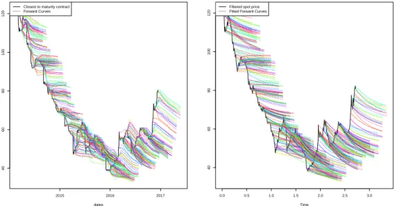
alumina concentration case study. . . 47 4–1 The solid black line represents closest to maturity daily Iron
Ore 62% Fe, CFR China contracts, which can be interpreted as a proxy for TSI index level (or spot price). For each trading day, forward curve is extracted for contract maturing in the next year. The graphic is generated using the Schwartz 97 R package (Erb et al., 2014) . . . 58 4–2 Iron Ore 62% Fe, CFR China contracts, TSI index level . . . 60 4–3 Training (above) and prediction (below) partitions for the iron
ore time series. The histogram represents the distribution of log returns. The blue line is a kernel density estimation (kde) plot using a Gaussian kernel and the dashed green line represents a normal distribution with the theoretical mean
and variance presented in Table 4–1. . . 66 4–4 Aggregated volume from all contracts for the prediction
parti-tion of the iron ore futures time series. . . 67 4–5 The top plot represents a heat map of traded volumes in
func-tion of maturity and date. Red color indicates highest traded volumes. The bottom plot represents the sum of volume of all contracts for a given maturity. Nearest maturities have
4–6 Left plot shows nearest actual contracts (black line) as well as future curves for each trading day in the studied period of time. The right plot shows the fitted corresponding variables estimated with Kalman filter. . . 70 4–7 Simulated paths (in gray color) with parameters derived from
the MLE algorithm. The continuous red line represents the mean of all the simulations and the red dashed lines represent the 95% confidence interval. The continuous green line is the actual price. . . 71 4–8 Kernel density plot of residuals for the first five maturing
contracts. . . 72 4–9 Histograms of NPV for the three different scenarios. The
neutral scenario is in blue, while the bullish and bearish
scenarios are respectively in green and in red. . . 73 4–10 NPV with a varying proportion of production sold in futures
markets. The analysis is performed for the optimistic, neutral and pessimistic price profiles in futures markets. . . 75 5–1 Simulated time series containing 259 observations. Plot a)
shows the long-term price index as well as the sum of the long-term price and short-term deviations. Plot b) shows simulated commodity contracts with maturities of 1, 5, 9, 12 and 17 months. . . 98 5–2 Time to expiration of crude oil contracts aggregated from
Quandl API. The time series ranges between 1990-01-02 and 1995-02-17. Contracts are expiring up to 17 months in the
future. . . 100 5–3 Crude oil futures contracts aggregated from the Quandl API.
For each trading week (time t), contracts are expiring at 1, 5, 9, 12 and 17 months into the future. . . 101 5–4 Convergence of the GA. The blue line represents the average
fitness of the population at each generation. The red line represents the solution within the population having the
highest fitness. . . 103 5–5 Plot a) represents the t+1 month crude oil contract (in blue) as
well as the KF estimate of the t+1 future contract (in green). The long-term price estimate of the KF is represented in red. Plot b) represents residuals (in %) of the KF estimates for
5–6 Plot a) of the Figure represents the t+1 month copper contract (in blue) as well as the KF estimate of the t+1 future contract (in green). The long-term price estimate of the KF is represented in red. Plot b) represents residuals (in %) of the KF estimates for each maturing contract. . . 108 5–7 Plot a) of the Figure represents the KF estimate of the
long-term trend and the estimated spot price. Plot b) represents simulation of copper contracts for the calibrated SSTF model. Plot c) represents the size of the stockpile, conditional on difference between estimated spot price and the long-term
trend. . . 111 5–8 Value added (alpha) of the active trading strategy compared to
the basic NPV investment. Alpha is calculated by differencing NPV using an active strategy to passive NPV for each
simulation outcome. . . 112 6–1 Price levels for gold, silver, platinum (in $USD/ounce) and
crude oil futures (in $USD/barrel) during 8 February 1993
and 8 November 2016. . . 129 6–2 Logarithm of returns of gold spot prices during 8 February
1993 and 8 November 2016. The first period ranges between 8 February 1993 and 27 December 2004. The second period ranges between 29 December 2004 and 8 November 2016. . . 130 6–3 Boxplots for gold, silver, platinum and crude oil futures price
returns. The points are considered as outliers when the
distribution is assumed to be normal. . . 132 6–4 Histogram of spot gold price returns. The dashed PDF
cor-responds to a normal distribution with the same mean and variance as observed in the empirical dataset. The continuous PDF is calculated with a kernel density estimator. . . 133
CHAPTER 1 Introduction
1.1 Overview
The valuation of a mining project requires assessing risk such as market, operational, geological, political and environmental risk. To assess the geo-logical risk, workflows involving stochastic modeling of an ore body followed by its production schedule optimization to determine future production rates have proven to be very promising. However, when converting forecasted pro-duction rates into cash flows, forecasted spot prices of a commodity also have to be taken into account.
The Net Present Value (NPV) approach is widely used to assess the present economic value of a mining project over its entire life. The approach consists in projecting future cash flows and then discounting them with a rate reflecting the risk of the investment. Discounted cash flows are then summed and compared to the initial expenditures required to undergo the mining project, and if the difference is positive, the project should be ac-cepted. However, mining projects can often last more than ten years, a period where cycles, jumps and spikes will influence commodity prices. These changes in prices will greatly influence forecasted cash flows, affecting the value of a mining project. Moreover, choosing the right discount rate to calculate NPV may be very subjective. A too small discount rate may make an unviable project look profitable while a too big discount rate may underestimate cash outflows needed for the completion phase of a mining project. Finally, man-agerial flexibility is not addressed when performing NPV valuation. For these
reasons, the NPV valuation technique may be too rigid to reflect the true complexity of a mining project.
A promising and increasingly popular approach for valuing mining projects is the Real Options valuation (ROV). This method of valuation is similar to NPV valuation in the sense that present and future cash flows are discounted and summed to value an investment. The difference is that the management team of a mining project are given options, for example, to mothball, close, open, accelerate or pause a project. Also, instead of affecting a project di-rectly, managers are given options to hedge their production using options or future markets. This increase in flexibility adds some value to a mining project but can be hard to put in practice because of the costs associated with changes in the project. However, when commodity markets are subjected to extreme events such as spikes or strong cycles, ROV may be necessary as a complementary approach to NPV.
Workflows based on ROV are usually implemented in a Monte Carlo (MC) simulation framework. The general MC framework requires modeling differ-ent scenarios of spot prices using a stochastic process. The parameters of the stochastic process may be calibrated on historical data or inferred from the knowledge of the modeler. If the historical approach is chosen for the calibra-tion, the stochastic process parameters are adjusted to reflect price dynamics in the recent past. The Kalman filter has proven to be a very useful tool for the calibration of stochastic processes on historical data. When using the Kalman filter, the stochastic process is written in a state-space representation which decomposes the process into two parts: the transition equation and the measurement equations. The transition equation is the true process while the measurement equation is the measured process. The measurements are usually noisy. A maximum likelihood routine can be used to adjust the parameters
governing the transition equation to better fit historical data. The procedure consists of applying the Kalman filter on historical observations with a vector of parameters and computing the logarithm of likelihood estimate. Then, an optimization routine is used to adjust the vector of parameters to maximize the likelihood. In practice, this procedure is converted to a minimization problem by taking the negative of the likelihood.
The optimization of the parameters of the Kalman filter is a major task in this thesis. Usually, the optimization routines used to perform the calibration are gradient based and can be stuck in a local minimum. To overcome this problem, several different starting values can be tested to ensure the conver-gence to a global minimum. However, a better approach is to use a different class of optimization routines that can handle non-linear and multidimensional cost functions. Namely, in this thesis, the use of a genetic algorithm and a particle swarm optimization are tested for the calibration of historical param-eters. This class of algorithm mimics the behavior of nature to solve problems. In the case of the genetic algorithm, the theory of evolution is implemented in the algorithm. The particle swarm optimization mimics how swarm of in-dividuals in a herd collaborate to survive. In any case, several solutions are tested at each iteration and the likelihood to get stuck in a local extremum thus is diminished.
Once the parameters of the stochastic process have been calibrated, they can be used to perform simulations. An active trading strategy using the Kalman filter and the Schwartz-Smith two-factor (SSTF) model is tested. The SSTF makes the assumption that the price of a commodity can be decomposed into two different terms. The long-term price is expected to evolve following a (geometric Brownian motion) GBM while the short-term price is mean-reverting. The application of the active trading strategy is implemented using
both price components in the SSTF. When the short-term price drives the spot price lower than implied by its long-term trend, a percentage of the production of a mining project is stockpiled for later use. When the short-term price drives the spot price higher, a part of the production that was previously stockpiled is sent to the market. This mean-reversion strategy can increase the NPV of a mining project by 5% to 10%.
Another use of the Kalman filter calibration workflow is to assess the market risk of a mining project. The commodity returns are generally better fitted with a fat-tail distribution. This is due to the fact that prices can jump or be affected by volatility clusters. These features are not well captured by the GBM. On another hand, the Merton jump (MJ) and Heston stochastic volatility (SV) model are able to reproduce behavior observed in the mar-kets. The use of the MJ and SV models for the calculation of cash-flow at risk (CFaR) are investigated. These stochastic processes are better suited to reproduce fat-tails and provide a value of CFaR which is more conservative than the GBM.
The next section lists the different publications associated with this thesis. 1.2 Original Contributions
The first part of the project is to apply robust regression algorithms on a dataset containing outliers. One must be very careful before deleting outliers from a dataset since they can be good data points that may have resulted from an extreme case of the sample generating process, or perhaps a secondary process. Several tools exist to detect and calculate the influence and leverage of outlier points. Then, using robust regression estimators, parameters from the regression can be estimated without any bias. The work done in robust regression has led to the publication of an article called Analysis of mining engineering data using robust estimators in presence of outliers, in the Natural
Resources Research Journal. The original contribution of this paper is the development of a workflow capable of detecting outliers and downsizing them to reduce the effect on regression models. The tools developed in this research are later used to detect abnormal jumps in the distribution of commodity returns.
The second publication uses a new approach using long-term commit-ment contracts (LTC) and futures contracts to value iron ore projects. This approach supposes that the management team of the iron mine has the ability to use two types of financial instruments to sell their production. The first in-strument is the long-term commitment contracts and the second inin-strument is the futures contract which can be traded in financial markets. The long-term instrument is considered as a risk-free instrument, while the futures contract is actively traded and fluctuates. The Kalman filter is used to estimate the dynamics of futures contracts, iteratively predicting unknown observations, then updating the parameters to improve the next prediction. The Kalman filter is the ideal estimator when the transition equation is linear and when the residuals are following a normal distribution. However, iron ore markets are subject to extreme events, such as jumps, which cannot be considered linear. These jumps are generally followed by an increase of volatility in markets. The first objective of this paper is to improve the Kalman filter estimates by scal-ing the observation uncertainties with the volume of traded contracts. Then, simulations of iron ore prices are performed with correctly calibrated param-eters. Results show that this workflow can be used to adjust the proportion of the productions sold using LTC or futures contracts according to the risk appetite of the company. Results show that the calibration and NPV simu-lation workflow can be effectively used to assess the profitability of a mining project, accounting for the exposure in futures markets.
The third publication uses a genetic algorithm (GA) to calibrate the pa-rameters of the Schwartz-Smith two-factor (SWTF) model on oil and copper futures contracts. Usually, the optimization is done using a deterministic opti-mization called the Expectation-Maxiopti-mization (EM) algorithm which can get stuck in a local maximum. Although they are slower than EM algorithms be-cause they use random number generators to search for the optimal solution, genetic algorithms optimize a population of solutions instead of working on only one solution at the time. Moreover, a constraint on the range parameter can be applied to ensure the parameter has a sound economic meaning. To demonstrate the performance of the proposed approach, a case study was con-ducted on a copper deposit. The simulations were based on the SWTF model whose parameters are determined by GA . An active management strategy of the stockpile, dependent on discrepancies in commodity futures prices is tested. Results show that the active management strategy produces positive returns over the passive investment approach.
The last publication compares several models used for the estimation of the CFaR of a mining project. The model parameters are calibrated using the Kalman filter. Then, Monte-Carlo simulations using the calibrated parameters are performed to compare the stochastic volatility model, the Merton jump diffusion process, and the geometric Brownian motion when assessing market risk exposure of a mining project. The contribution of this research is to provide a robust workflow to calibrate commodity price dynamics models to historical data using the Kalman filter. The parameters of the model are fitted using a particle swarm optimization routine combined with a gradient-based search method.
CHAPTER 2 Literature Review
2.1 Overview
In this section, an extensive literature survey on the concepts tackled in the thesis is presented. The literature survey revolves around the concept of options pricing in financial markets and its extension to a Real Option frame-work. Other concepts, such as genetic algorithms and the Kalman filter are introduced because they can be used to simulate or derive unknown parame-ters in stochastic process models.
The first section discusses risk related to commodity markets and strate-gies to protect a mining company from that risk. First of all, some basic concepts about the mining industry are covered. After, some basic manage-ment concepts on mining projects are covered. These managemanage-ment strategies involves option and futures contracts and are designed to reduce volatility in quarterly earnings of mining companies. Then, a review of how volatility fore-casting models have been used to forecast volatility of commodity prices is made. These commodities include petroleum and minerals, but also agricul-tural commodities such as soybeans, and wheat.
The second section introduces robust regression as a tool for outlier detec-tion and mitigadetec-tion. It is well documented that financial markets are subjected to crashes. These extreme movements cannot be modeled with the normal dis-tribution and will generally make the conventional statistical estimates biased. For this reason, another class of robust statistics models was introduced. One of the main tasks when treating for outliers in a dataset is to detect them. A
review of outlier detection methods is made as well as a review of robust esti-mation techniques. These tools are used later in this thesis to accommodate for outliers in commodity market returns.
The next section introduces some stochastic processes used to generate simulations in stock, bonds, commodities and futures markets. Stochastic processes are very useful to simulates possible price paths and assess how a mining project can be affected by the market fluctuations. Another popular use of these stochastic processes is to assess market risk of mining projects. Then, it is possible to estimate how a hedging program can help to mitigate this market risk. A variety of stochastic processes exists in the literature. Some, like the geometric Brownian motion, are more parsimonious in terms of the number of parameters to estimate. Other models have more parameters constraining the stochastic process. Each stochastic processes have their own advantages and inconvenient and they should be chosen in function of the problem to be solved.
The fourth section introduces the state space representation of stochastic processes and the Kalman filter. The Kalman filter is a very powerful tool used for the simulation of stochastic processes as well as for parameter estimation. Once a stochastic process has been represented in its state space form, it is possible to estimate its transition equation using the Kalman filter. In this thesis, the Kalman filter in a central topic because of its flexibility. However, it can be difficult to calibrate the Kalman filter with historical observations because the optimization routine can yield to infeasible parameters estimates. For this reason, genetic algorithms were used for the calibration of the Kalman filter.
The next section introduces genetic algorithms. The genetic algorithm is a metaheuristics approach which is particularly suitable to solve non-linear
problems. When the objective (or cost) function of an optimization problem contains multiple dependent parameters and the landscape of this function is irregular with multiple local minimums, the genetic algorithm probes to be superior to the steepest descent approach for optimization. This is due to the fact that genetic algorithms work with a population of points to estimate instead of working on a single optimization point at a time. A tradeoff of using the genetic algorithm is computation efficiency.
The sixth section introduces pioneering work as well as recent work on option-pricing theory. With a calibrated stochastic process (using the Kalman filter and genetic algorithm workflow), it is possible to perform simulation and to estimate the value of derivatives contracts dependent on price path simulations of commodities, stocks or bonds. Then, an extension from the valuation option-pricing theory to Real Options valuation is presented. Real options are useful to determine the value of managerial flexibility in a capital budgeting projects. For example, the real option to close a mining project when the commodity price is unfavorable may add value over the alternative status quo (or doing nothing). A parallel can be made between real options and financial options. For example, closing a mine project can be seen as a financial put option: the assets are sold at a given price and the project is terminated. The last section presents how Real Options valuation can be applied to the valuation of mining projects.
2.2 Market risk regarding commodity markets
The mining industry can be separated into three principal spheres: ex-ploration, mining and metallurgy (Svetlana, 2010). Each sphere is affected by mineral market fluctuations. For example, in a mineral boom, exploration companies are getting a lot of liquidity to rapidly find the next ore deposit in order to bring minerals on the market while mining companies may try
to acquire smaller mines or boost their already existing production. For this reason, valuing mining companies is difficult due to the impact of mineral and economical cycles (Svetlana, 2010). The first cyclical effect refers to the fact that the value of the commodity company is not only affected by the price of the commodity but also by the expected volatility in that price, leading to higher volatility in earnings than other sectors in the market. The second cyclical effect refers to the high fixed operating costs of mineral extraction projects; because of these high fixed costs, mining companies need to keep their operations active even in economic downturns. Another important as-pect of mining companies is that ore deposits have a finite geometry meaning that if mining companies do not invest in exploration campaigns or acquire other mining properties, they are condemned to disappear (Svetlana, 2010).
Once the fact that mining companies are subject to some cycles has been established, several questions need to be answered. First of all, how are such types of companies going to be managed? The basic management problem can be stated very simply. The prices of commodity metals fluctuate by large amounts from one period to another, whereas costs are relatively more stable, resulting in large profit instability (Adams, 1991). Financial markets tend to give more valuation to companies with stable earnings since they are pre-dictable. What tools can mining company’s managers use to stabilize earnings throughout the life of a (or a portfolio of) mining project(s)? In his research, Adams (1991) denotes three principal management strategies to get through downward mining cycles: Capital repayment reduction, restructuring net op-erating costs and risk sharing. The first strategy is to reduce the fixed re-payment schedule by offering metal loans (i.e. a gold loan) or bonds. The second strategy involves varying volumes of production and margins during mining cycles in order to stabilize the earnings; hence increasing stability at
the cost of profitability. The last strategy involves hedging potential losses by offering futures contracts to buyers of the produced commodity. In all cases, such strategies need to be implemented before downward cycles start.
Commodity prices have always been very volatile and hard to predict. Kroner et al. (1995) were among the first researchers to use econometric models to perform long horizon (up to 225 days) forecasts of volatility on commodity markets. To do so, they forecasted volatility using expectations derived from options prices (market expectation or presumed volatility forecasts), forecasts using time series modeling, and forecasts with a combination of market expec-tation and time-series methods. Kroner et al. (1995) showed that the workflow using a combination of implied and realized volatility gives the best results over the two other workflows. The reason why the combination method is better than the others is that options markets are inefficient. Econometric models were later used to forecast volatility in agricultural commodities such as corn, wheat and soybeans (Manfredo and Leuthold, 1998). According to the au-thors, value at risk (VaR) and GARCH forecasting appears to be a promising management tool for the agricultural industry, since it can quantify exposure to market risk of cultures and provide incentives to develop hedging strategies. Giot and Laurent (2003) used econometric models such as RiskMetric, skewed Student APARCH and skewed Student ARCH to predict value at risk of long and short positions in commodities markets. APARCH models can account for the tails asymmetrical distribution, allowing more weight on past negative returns than past positive returns. Also, since the authors use a Student dis-tribution, they can account for fat tails, thus, he is able to better reproduce strongly negative returns. The authors showed that the three methods could be used to do very short-term predictions (1 day predictions). In most cases, RiskMetric failed to predict VaR 1 while skewed Student APARCH gave the
best predictions. However skewed Student ARCH is a good compromise since there is no need to perform non-linear optimizations in the procedure. It is not sure if econometric models bring an added value over forecasts of supply and demand for long-run predictions, but the methodology could definitely be implemented to perform midterm predictions (Giot and Laurent, 2003). Later, Sadorsky (2006) used econometric principles to forecast volatility in petroleum markets. The data used for his study were observations on the daily closing futures price returns on West Texas Intermediate crude oil, heating oil #2, unleaded gasoline and natural gas from the 1988-2003 period. The time pe-riod of the study makes the evaluation of econometric models very robust since oil prices were affected by large fluctuations during that period of time. The conclusion of this study was that a TGARCH model fits well for heat-ing oil and natural gas volatility and a GARCH model fits well for crude oil and unleaded gasoline volatility. Then, non-parametric value at risk measures based on volatility forecasts of oil and gas markets can provide a useful way to measure risk exposure of an investment in oil and gas commodities (Sadorsky, 2006).
Since datasets can be contaminated with outliers, it is important to detect them and when possible, treat them with robust statistical methods. The next section introduces robust regression.
2.3 Robust regression
Before introducing stochastic processes, it is important to understand that any dataset can be contaminated with outliers. Outliers are different from bad data in the sense that they may be extreme values of a generation process or they can perhaps be generated from a secondary process (Ortiz et al., 2006). Several methods can be used to detect outliers. These methods are often based on distance measures or analysis of clustering. There is also
a distinction between the univariate and multivariate case. In the first case, there is no covariance term to calculate between the different variables. As a result, a simple method like the studentized residual method can be used to detect outliers (Thompson, 1935). In the multivariate case, it is often more useful to use a distance measure to detect outliers. For example, Filzmoser et al. (2005) used the Mahalanobis distance to assess which data points can be considered as outliers in a regression plot. This method is suitable for a multivariate case because it does not assume the distribution of the data.
Once the outliers are detected, they can be corrected using robust regres-sion. Huber (1973) introduced the M-regression based on maximum likelihood. This estimator has the advantage to be very efficient. Rousseeuw (1984) intro-duced the least-median square (LMS) which is less affected by the presence of outliers. The LMS regression method is a particular case of quantile regression (Powell, 1986). A least-trimmed square estimator is useful when the dataset is contaminated with a substantial amount of outliers (Leroy and Rousseeuw, 1987). Yohai (1987) proposed a high breakdown point and highly efficient ro-bust estimator called the MM-estimator. The MM-estimator has the highest breakout point possible of 0.5 meaning that up to 50% of the dataset can be contaminated by outliers before the robust estimator breaks.
Outliers will often appear in financial time series so it is important to understand how they can affect different estimates. Martin and Simin (2003) showed how outliers could affect estimates of betas used in the Capital Asset Pricing Model (CAPM). Authors propose an alternative approach than OLS to calculate betas. This complementary approach can also be coupled with the traditional calculation of beta to detect outliers. Robust methods can also be used to model operational risk in financial institutions and help to characterize how they can be affected by outlier events Chernobai and Rachev
(2006). The aim of using robust regression is not to discard extreme events but rather to partition a dataset in an outlier-free and outlier contaminated sets. This results in a much more meaningful analysis of time series since the estimates are not biased by a few but extremely influent outlier points. Robust statistics in finance can also be used to construct portfolios resistant to outliers (Welsch and Zhou, 2007). Results show that robust portfolios have a lower asset turnover and an increased risk adjusted return.
Some stochastic processes are better suited to deal with outliers. The following paragraphs, a review the different stochastic processes.
2.4 Stochastic processes
Samuelson (1965) introduced the first stochastic process models used to estimate returns in financial markets. The author used geometric Brownian motion (GBM) to describe how financial returns could evolve between two points in time using a drift and a volatility parameter. It was shown that in GBM diffusion models, financial returns are independent from previous returns (Samuelson, 1965). Stochastic interest rates tend to grow indefinitely when applying simple GBM to model them (Vasicek, 1977). Instead, an Ornstein-Uhlenbeck process is introduced in the diffusion process to describe the short-term rate dynamics.
Stochastic volatility (SV) methods were later developed to overcome the strong constant volatility assumption in previously developed diffusion model. Andersen and Shephard (2009) published an exhaustive literature review on stochastic volatility. They made a clear distinction between SV methods and ARCH based methods (often confused for SV methods). In stochastic volatility methods, the conditional likelihood function is not known as opposed to one-step-ahead predictions such as ARCH. In SV, the asset returns are instead approximated by a mixture distribution where the level of activity of new
arrivals is taken into account. The Heston SV (Heston, 1993) model links these biases within the Black-Scholes (BS) model to the dynamics of the spot price and the distribution of spot returns. The author shows that even if the BS model produces option prices similar to the stochastic volatility models for at-the-money options, SV models are better suited to explain skewness of option spreads by modeling the correlation between volatility and the spot price. Merton (1976) used a different approach and introduced an independent jump component to the GBM. As a result, the stochastic process is able to reproduce outliers that can’t be modeled with the GBM. Later the work of Bates (1996) extended the Heston model and the Merton jump by combining both stochastic volatility and jump components. Bates (1996) shows how these jumps are important for modeling options prices simultaneously across the strike and time-to-maturity spectrum.
The convenience yield has to be taken into account when modeling dif-fusion processes governing different commodities. Unlike stock markets, com-modity markets are accompanied with forward and future markets which can provide insights of future prices (Geman, 2005). Because of the high level of similarities between forward curves in commodities and yield curve in bond markets, theories developed in the fixed-income field in finance have been ap-plied to model commodities (Geman, 2005). Schwartz (1997a) compares three models that take into account mean reversion. In the first model, a one-factor model following a mean-reverting process governs the diffusion process. The second model is a two-factor diffusion model taking the stochastic convenience yield of a commodity as a factor. The third model is a three-factor model that also includes randomly varying interest rates. Casassus and Collin Dufresne (2005) showed how the convenience yield could be modeled using the Schwartz three-factor model.
There is a fundamental difficulty in historical volatility forecasting: volatil-ity is not directly observable (Dan`ıelsson, 2011). In other words, to detect volatility increases, one must first observe changes in price ranges to volatility changes to occur. For this reason, volatility is called a latent variable, which means there is a delay between the present time and volatility. However, there is an exception to this observation. For example, futures on volatility indices such as the VIX from the Chicago Board Option Exchange are based on the spread on future options, which means volatility forecasting is based on fu-ture values of implied volatility (Alexander, 2008). For this reason, such an approach is called implied volatility forecasting (Christensen and Prabhala, 1998). Day and Lewis (1988) observed that when approaching the expiration date for stock index options, volatility tends to increase significantly. Stud-ies on implied volatility forecasting are based on the idea that option spread should reflect realized volatility given the fact that option markets are efficient. The very first method used for historical volatility forecasting was the simple moving average (SMA). Volatility forecasts are based on returns on past days of trading (Dan`ıelsson, 2011). Since volatility tends to cluster, it is important to have a volatility forecast method which puts more weight on recent observations. The SMA volatility forecast tend to underestimate volatility because it applies equal weight to each trading day. For this reason, Morgan (1996) released a publicly available volatility forecasting model called the Exponential Weight Moving Average (EWMA), also called RiskMetric. The difference between SMA and EWMA is that the latter method applies an exponentially decreasing weight from the most recent days of trading to the preceding days. One can choose the decay factor of the EWMA calculation which is a number between 0 and 1. Morgan (1996) suggests to use 0.94 as
a decay factor for all types of investment securities, which is a subjective but suitable value of decay.
The volatility forecasting models discussed in the previous paragraphs were univariate. Extending the theory to take into account several assets at the same time is not always an easy task, since the covariance between different assets needs to be calculated (Dan`ıelsson, 2011). One of the firsts multivariate model developed was the BEKK (Engle and Kroner, 1995) where the matrix of conditional covariances is a function of the product of lagged returns and lagged conditional covariances, constrained by a parameter matrix. Another approach to model multivariate data is to assume that the observed data can be linearly transformed into a set of uncorrelated components using an inversion matrix. Parameters of the inversion matrix depend on conditional information which can be calculated directly from time series.
Another family of volatility forecasting methods is the Stochastic Volatil-ity (SV) (Dan`ıelsson, 2011). This family of methods uses random number generation to generate equiprobable scenarios of volatility constrained by an input model. Also, SV models differ from ARCH based models where the con-ditional variance of returns is given by past returns observed, while in the SV approach the predictive distribution of returns is specified indirectly, via the structure of the model (Andersen and Shephard, 2009). In SV models, price changes are due to exogenous shocks to the stochastic distribution of returns. The stochastic features of time series have been observed for a long time in the literature. Mandelbrot (1963) describes a succession of returns with the random walk theory, where returns have a Brownian motion.
This family of forecasting methods was developed to overcome the strong normal distribution assumption in the BS option pricing model (Heston, 1993). The Heston SV model links these biases within the BS model to the dynamics
of the spot price and the distribution of spot returns. The author shows that even if the BS model produces option prices similar to the stochastic volatil-ity models for at-the-money options, SV models are better suited to explain skewness of option spreads by modeling the correlation between volatility and the spot price. Later Bates (1996) extended the Heston model to allow for jumps in volatility. Bates (1996) shows how these jumps are important for modeling option prices simultaneously across the strike and time-to-maturity spectrum.
Brennan and Schwartz (1985) were the first to introduce a model that infers a relationship between commodity spot prices and futures. To link these two aspects, they introduced the convenience yield which is a continuously compounded benefit taht the owner of a forward or futures contract renounce to when buying the contract. The greater the convenience yield is, the lower the fair value of the contract is. In Brennan and Schwartz (1985), the spot price moves according to a geometric Brownian motion (GBM) with deterministic convenience yield and risk-free interest rates. Later, Gibson and Schwartz (1990) used the the previous models and tested a two-factor model for pricing weekly oil futures contracts using spot price and the instantaneous convenience yield as variables.
A very useful algorithm for calibrating stochastic processes is the Kalman filter (KF). The next section introduces the KF and its diverse applications for solving engineering problems.
2.5 State space representation of stochastic processes
The KF was introduced in 1960 and have found numerous applications in solving engineering problems (Kalman et al., 1960). One of the first important uses of the KF was to implement the recursive algorithm responsible of tracking the Apollo spacecraft and its lunar module (Willems, 1978). The KF separates
a signal into two different partitions. The measurement partition contains measurement errors and can be used to estimate the transition equations, which describe the phenomenon to be modeled. For example, in the case of a radar measurement, the position of a vessel can be measured with a certain amount of noise, but the instantaneous velocity needs to be inferred from different subsequent measurements of position (Brookner, 1998). In this case, the transition equations will describe how velocity is related to position and the measurements will be used in the KF to estimate the correct velocity.
A wide range of engineering problems can be solved using the KF. More-over, the KF can be used to solve engineering problems containing multiple independent variables or in multiple dimensions. For example, the KF can be used to track objects in 3 dimensions using the Global Positioning System (GPS) (Sasiadek et al., 2000). More recently, the KF have been widely used to track Unmanned Aerial Vehicles (UAV), also known as drones (Benini et al., 2013). The previous examples showed how the KF could be used for tracking objects in multiple dimensions. Another important use of the KF is for the interpretation of sensor measurements used in automated processes. An ex-tension of the KF, the Ensemble Kalman filter (EnKF), can be used to solve engineering problems related to geology and geography (Evensen, 2003). Ben-ndorf et al. (2014) used the EnKF for the real-time online characterization of properties of coal moved on conveyor belts. The workflow enables the recon-ciliation of the geostatistical model and actual measurements of the material properties. The extended Kalman filter (eKF) fas introduced to solve problems where the transition equations are non-linear (McElhoe, 1966). The method uses Tailor series expansions to linearize the problem. Other approaches can be used to describe non-linear problems. The particle filter (PF) was intro-duced to overcome the linearity assumptions of the KF (Del Moral, 1996). The
PF is more accurate than the KF when the problem is non-linear but since it relies on the estimation of discrete particles instead of a normal distribution assumption of the error term, it is more computationally intensive.
The KF and its derivatives methods can be used to infer hidden state variables from commodity futures contracts observations. Schwartz (1997a) introduced the state space representation of stochastic processes in the con-text of commodity futures estimation. The author compared three models that took into account mean reversion in the convenience yield. In the first model, a one-factor model following a mean-reverting process governs the diffusion process. The second model is the Gibson and Schwartz (1990) model. The third model is a three-factor model that also includes randomly varying in-terest rates. In order to correctly estimate parameters, Schwartz (1997a) uses KF techniques to continuously and iteratively correct the covariance matrix. Ribeiro and Hodges (2004) further extended the long-term Schwartz two-factor model by replacing the Ornstein-Uhlenbeck by a Cox-Ingersoll-Ross to model the convenience yield. This ensures that the model is arbitrage free. Further-more, they examined the spot price volatility as proportional to the square root of the convenience yield level.
Both Ribeiro and Hodges (2004) and Schwartz (1997a) models are adept at pricing short-term contracts, but fail when pricing longer term structures. Schwartz and Smith (2000a) eliminated the concept of convenience yield and modeled the log of the spot price as the sum of a short and a long-term component. The model allows mean reversion in the short-term and uncer-tainty in the long-term price. Movements in prices for long maturity futures contracts describe the long-term equilibrium level and the difference between short-term contracts and long-term describes how spot prices mean revert in
the short-term. This specification is better at pricing longer term futures con-tracts than previous models. Aiube and Samanez (2014) reconducted analysis in oil futures markets using longer maturity contracts that were not available in previous studies. Authors showed that the use of these multifactor models tend to underestimate the risk premium observed in futures prices.
The KF is very useful to estimate commodity markets dynamics. How-ever, calibrating the parameters can be challenging. In this thesis, the use of the genetic algorithm for the calibration of the Schwartz-Smith model (Schwartz and Smith, 2000a) is investigated. The next section presents a brief literature survey on genetic algorithms.
2.6 Genetic algorithms
Genetic algorithms (GAs) appeared in the mid 70’s with the pioneering work of Holland (1975). In the first formulation of the GA, a set of param-eters to be optimized were encoded using a binary representation. GAs can ignore the gradient of the optimized function since they rely on an objective function to evaluate the transition from a solution to another. This enables the algorithm to consider a population of points instead of focusing on the gradient optimization of a single point which can be stuck in a local maximum (or minimum) (Goldberg and Holland, 1988). This makes the GA particu-larly suitable to optimize highly non-linear functions. As a result, GAs are employed in a wide range of engineering optimization problems.
Some researchers have used the GAs to literally simulate the evolution of virtual creatures (Sims, 1994). The authors have created a 3D virtual en-vironment subject to physical constraints and used the GAs to simulate the evolution of randomly generated creatures. The objective function represented tasks the virtual creatures were required to perform such as jumping, swim-ming or walking. The GAs helped to design complex morphologies that were
optimal for performing the tasks. Later, GAs were used for the optimization of the shape of the wing of an aircraft (Obayashi et al., 2000). In this case, the shape of the wing could be modified iteratively to have better aerodynamic characteristics.
In the previous examples, GAs were used to optimize the shape of com-puter generated objects. GAs are also suitable for solving abstract engineering problems. Mahfoud and Mani (1996) used the GA to forecast individual finan-cial stock performance. The authors used the GAs to model how the combina-tion of 15 attributes can be used to forecast favorable market circumstances. Later, Shin and Lee (2002) used the GA to predict bankruptcies of Korean financial institutions. The GA can have multiple objectives to optimize at the same time. Tapia and Coello (2007) denoted five types of problems that are solved using multi-objective GA optimization. The five types of application are: investment portfolio optimization, financial time series modeling, stock ranking and screening, risk-Return analysis and economic modeling.
Other algorithms use behavior observed in nature to solve problems. Eberhart and Kennedy (1995) introduced particle swarm optimization (PSO). This algorithm mimics how a herd of individuals cooperate to better sur-vive. Each individual is allowed to move independently at a given speed. The swarm collectively knows which solution is the best, but individual member of the swarm move randomly to try to find a better solution. Maniezzo (1992) introduced ant colony optimization (ACO), which mimics the behavior of an ant colony which tries to optimize the route between their colony and a source of food.
Any of the presented metaheuristics approaches can be used to optimize the KF parameters. Ting et al. (2014) used the GAs to optimize the parame-ter of the KF in a batparame-tery management system. Authors show the methodol-ogy is suitable because it produces low root mean-square (RMS) error values. Ortmanns et al. (2015) used a combination of GA and unscented Kalman fil-ter (UKF) for the estimation of paramefil-ters used in a sigma-delta modulator analog-to-digital converter. Luis Enrique Coronado (2015) used a combination of extended KF and GAs for the optimization of neuro-mechanical parameters responsible to prevent human from falling. The workflow is better suited than actual trial and error methods for finding a solution to the problem.
The next section introduces options pricing theory. This will be useful to better understand real options, a central concept in this thesis.
2.7 Options pricing theory in financial markets
An extensive literature survey exists in the valuation of options traded in financial markets. Black and Scholes (1973) developed a widely used formula to price European-style options. The BS formula takes a stock price, the option exercise price and its time to expiration, the risk-free interest rate and the volatility as an input and computes the price an investor should pay for that option. In the BS formula, stock price returns obey a geometric Brownian motion, and they follow a log normal distribution. Moreover, in BS formulation, the volatility is constant. It is well known that these assumptions are not true because volatility tends to be clustered in periods of high and low volatility (Fama, 1965). If a stock price can be modeled as a GBM affected by shocks such as important news or political decisions, volatility should also be affected by these shocks (Fama, 1965).
Later, Merton (1976) improved the BS model by allowing for stochastic jumps in the stock price returns while considering the volatility constant over
time. As a result, a premium has to be added to options where the stock prices are exhibiting strong changes in magnitude. Schwartz (1977) solved partial differential equations in the BS and Merton models to take account for dividend-paying stocks. A numerical example based on the pricing of American Telephone and Telegraph (ATT ticker) options comparing Schwartz model with BS without dividends and BS with dividends, show a discrepancy between real market prices of options and Schwartz model. According to Schwartz (1977), the discrepancy could be due to a bias in the model, a bias in the market value or a discrepancy in the historical variance derived to price the option using the model and the variance predominant in the market valued options. Cox et al. (1979) developed a numerical pricing option based on a binomial lattice. Their discrete-time approach uses simple mathematics and the no-arbitrage assumption in derivative markets. The binomial lattice method converges to the BS formulation when discrete time steps converge to zero. For this reason, the binomial lattice algorithm can be seen as a numerical implementation of the BS model.
Boyle (1977) later introduced a Monte-Carlo simulation approach in op-tions pricing theory. The approach uses computational power to generate a number of realizations of stock price return paths and has an advantage over analytic methods in cases where jump processes are present in the underlying stock price returns. Longstaff and Schwartz (2001) developed options val-uation with a Monte Carlo-based approach using least square regression to estimate the expected payoff of an option contract holder. The model is called the least square Monte-Carlo (LSMC) regression. Their method can calculate American type options, which is a significant advantage over methods that can only calculate European type options. Longstaff and Schwartz (2001) rec-ognized that using methods such as generalized methods of moments (GMM)
when estimating the conditional expectation function could lead to better re-sults when residuals from the regression are heteroscedastic. Jonen (2011) improved the LSMC algorithm for when the conditional expectation function contains outliers by replacing the least-squares estimator with a robust estima-tor. Jonen (2011) showed that the robust Monte-Carlo regression algorithm significantly reduces the bias without increasing the variance when using ro-bust loss functions such as Huber (Huber, 1973) in presence of outliers. Even if Monte-Carlo regression based techniques can tackle more complex problems by allowing for multiple simultaneous assets, stochastic volatility cannot be easily implemented because it would require solving a non-linear regression at each time step. In any case, analytical methods presented in this section are based on the assumption that volatility is constant over time, or non-stochastic.
The next section introduces real options, which is an extension of options pricing theory to the pricing of options on real assets.
2.8 Introduction to Real Options valuation
Because of the high level of similarities between management of a mine and the management of options traded in financial markets, Real Options val-uation was first introduced by Myers (1977) who made an analogy between an irreversible investment and a call option (or option to buy) in financial markets. An American call option can be exercised at any time before the ex-piration date. As an analogy, the possibility to undergo an irreversible invest-ment such as opening a mine can happen whenever after the completion of the feasibility study whenever the financial resources are available. At the project expiration date, financial actors may decide to invest their money elsewhere and the option to undergo the mining project expires. The added optionality using options pricing theory is referred in the literature as managerial flexibil-ity (Trigeorgis, 1993). In natural resource investment projects, management
teams have the possibility to defer or accelerate development, alter operating scale and abandon or temporarily close a mine (Trigeorgis, 1993).
Because Real Options valuation theory is based on an analogy with op-tions traded in financial markets, practitioners decided to adapt option-pricing theory in a Real Options framework. Copeland et al. (2001) made a compre-hensive book on applying Real Options valuation to real world problems. The authors are principally using decision tree analysis (DCA) with an approach similar to Cox et al. (1979) to value real financial assets as opposed to secu-rities. Luehrman (1998) considered characteristics of a real world investment problem as input variables into the BS model. For instance, present value of a project operating assets can be seen as the stock price, expenditures required to acquire the project assets are the call option exercise price, the period the decision can be postponed is the time to expiration, the time value of money corresponds to the risk-free interest rate,mean-reverting and the risk of the project corresponds to the variance of returns on stocks.
In the recent literature, several attempts have been made to apply Real Options to the valuation of mining projects. Even if the approach seems promising compared to the DCF approach, practitioners still have a lot of difficulties applying ROV to mining projects. One of the reasons is that ROV models are oversimplified and do not reflect the true complexity of a mining project investment (Dimitrakopoulos and Abdel Sabour, 2007). According to the authors, one of the major simplifications that render ROV impracti-cable is that production rates in a mine are considered to be constant. To overcome this difficulty, Dimitrakopoulos and Abdel Sabour (2007) focus on implementing a workflow integrating mine production sequence in the ROV framework. Another problem that is not currently well addressed in ROV