On the non-intrusive evaluation of fluid forces with the momentum equation approach

This is an author-deposited version published in:

http://oatao.univ-toulouse.fr/

Eprints ID: 13656

To link to this article: DOI:10.1088/0957-0233/20/9/095401

URL:

http://dx.doi.org/10.1088/0957-0233/20/9/095401

To cite this version: David, Laurent and Jardin, Thierry and Farcy, Alain

On the non-intrusive evaluation of fluid forces with the momentum

equation approach. (2009) Measurement Science and Technology, vol. 20

(n° 9). pp. 1-11. ISSN 0957-0233

O

pen

A

rchive

T

oulouse

A

rchive

O

uverte (

OATAO

)

OATAO is an open access repository that collects the work of Toulouse researchers and

makes it freely available over the web where possible.

Any correspondence concerning this service should be sent to the repository

administrator:

staff-oatao@inp-toulouse.fr

On the non-intrusive evaluation of fluid

forces with the momentum equation

approach

∗

L David, T Jardin and A Farcy

LEA, University of Poitiers, CNRS, ENSMA, SP2MI bd Marie et Pierre Curie, 86962 Futuroscope, France

E-mail:Laurent.David@univ-poitiers.fr

Abstract

The aim of this paper is to discuss the advantages and difficulties linked with the experimental application of the momentum equation approach as a non-intrusive way to predict the unsteady loads experienced by an airfoil in motion. First, in order to evaluate the influence of the varying parameters relative to the calculation of the corresponding drag and lift coefficients, numerical flow fields obtained by means of DNS are used. The comprehension of the impact of the spatial and temporal resolutions, velocity accuracy or third velocity component on the estimation of forces allows us to quantify the accuracy of the approach and helps in specifying the parameters setting which could lead to a consistent experimental application. In a second step, the approach is applied to experimental flow fields measured through the use of time resolved particle image velocimetry (TR-PIV). A low Reynolds number flow around an impulsively started airfoil is considered. The loads and vorticity flow fields are correlated and compared with those obtained by DNS.

Keywords: aerodynamics, lift, drag, momentum equation

(Some figures in this article are in colour only in the electronic version)

1. Introduction

Measuring the aerodynamic forces experienced by a body is of major interest when dealing with flow control applications, lift device optimization or energetic performance enhancement. Strain gauges are widely used for steady flow configurations whereas piezo-electric devices appear as an alternative solution for unsteady flow configurations. Nevertheless, such techniques are not universal as they are limited to a specific range of loads. Low Reynolds flows, as encountered in micro-air vehicles (MAVs) applications, cannot easily rely on these methods, the resulting aerodynamic forces being weak, hence leading to strong relative errors. Moreover, for specific applications (flow control with splitter element or with profile in motion, force measurement with more than one obstacle),

* This article is based on work presented at the EWA International Workshop on Advanced Measurement Techniques in Aerodynamics, held at Delft University of Technology, the Netherlands, 31 March–1 April 2008.

the devices begin to be somewhat complex and may present some drawbacks. Note that the integration of the surface pressure distribution can be achieved for the lift and pitching moment evaluation with pressure taps or pressure sensitive paint, and a pitot-tube wake rake could be used far downstream of the obstacle to determine the drag, as described by Jones (1936).

An alternative method is to deduce the unsteady forces from velocity flow fields by applying the momentum equation to a control volume enclosing the profile. The approach (Noca

et al 1997, 1999, Unal et al 1997) discussed in this paper allows non-intrusive steady (van Oudheusden et al2006) and unsteady (Kurtulus et al2007) loads measurement using the velocity flow fields determined by particle image velocimetry (PIV) and time resolved PIV, respectively. This method is particularly powerful in the sense that it permits a direct link between the flow behaviour and the force generating mechanisms, which is not a priori the case when separate

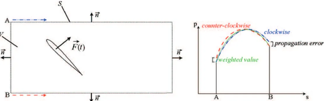
Figure 1.Control volume, surface definitions and pressure weighting process.

techniques are used to extract this information. Thanks to the recent development of high-rate imaging techniques, the momentum equation approach may be applied to relatively high Reynolds number configurations and is particularly convenient for low Reynolds flows. Furthermore, when a moving body is considered, the forces obtained through the use of gauges are the sum of both fluid and inertial forces. In other terms, the fluid forces are deduced by subtracting the inertial forces from the measured forces, increasing the relative error. Thus, the present method appears as a way to avoid such uncertainties.

In this paper, we focus on the practical application of the momentum equation using numerical and experimental data. The first part will present the concept of non-intrusive loads evaluation. The second part will discuss the influence of different parameters such as the spatial and temporal resolutions, velocity accuracy or the presence of a third velocity component using data obtained from a simulated flow. In the last section, loads evaluation will be applied to experimental data and compared with DNS results, leading to a concluding discussion.

2. Loads evaluation

Different approaches of the momentum equation can be proposed, based on the integration of flow variables inside a control volume surrounding a body. Lin and Rockwell (1996) apply the impulse concept, described by Moreau (1952a, 1952b) and Lighthill (1986), which needs the knowledge of the full vorticity field around the body. Starting an oscillating cylinder from rest, they study the flow field during the first instants in order to ensure the confining of the vorticity to a small domain close to the body. Later, Noca

et al (1997) suggest a solution based on the vorticity field in a finite control volume. By this means, the vorticity field does not have to be evaluated everywhere. The interest of this chosen formulation is the absence of the pressure term, eliminated from the momentum equation by algebraic manipulations. Furthermore, the authors mention the possibility of calculating only surface integrals. The approach is numerically validated and applied experimentally on an oscillating cylinder configuration. The comparison with the measurements by gauges reveals a bad agreement both on the amplitude and on the phase of the signal, justified by the two-dimensional approximation of the momentum balance

applied to a three-dimensional flow. In the same way, Protas

et al(2000) successfully implement their numerical flow solver with the approach proposed by Quartapelle and Napolitano (1982) in which the pressure term is eliminated by introducing a new variable depending only on the control volume geometry. Unal et al (1997) present an equivalent formulation which tends to minimize the evaluation of the spatial derivatives. In this case, the pressure term is calculated from the integration of the momentum equation. The experimental lifts (oscillating cylinder configuration) estimated by gauges, circulation measurements and momentum equation seem to be in good agreement despite some variations due to both three-dimensional effects and low spatio-temporal resolution. In a parametrical and numerical study, Noca et al (1999) show the insensitivity of the results to the dimension of the control volume and to the different approaches of the momentum balance.

As previously introduced, the approach discussed in this paper allows non-intrusive steady (van Oudheusden et al

2006) and unsteady (Kurtulus et al2007) loads measurement using the velocity flow fields determined by particle image velocimetry (PIV) or, respectively, time resolved PIV. The measurement of time resolved velocity flow fields reveals the unsteady behaviour of the physical structures. Moreover, the knowledge of the acceleration fields permits the application of the complete momentum equation approach to the velocity flow fields. The equation under integral form gives the instantaneous force EF (t )experienced by the airfoil in function of four components, E F (t ) = −ρ ZZ V Z _{∂ EV} ∂t dV − ρ Z S Z ( EV · En)( EV − EVs)dS − Z S Z p EndS + Z S Z τ · EndS, (1)

where En is the normal to the control surface S as shown in figure1, ρ is the fluid density, EV is the fluid velocity vector, EVs

is the control volume velocity and τ is the viscous stress tensor. The two first terms (unsteady and convective contributions) are directly deduced from the TR-PIV velocity flow fields. Note that the latter is not integrated over the airfoil surface since

E

V − EVs is null for a no through flow boundary condition.

In order to evaluate the third term (pressure contribution), pressure p along the control surface needs to be determined.

This flow property is obtained by spatially integrating the pressure gradient derived from the velocity flow field:

D EV

Dt = −

1

ρ∇p + ν∇

2_{V .E (2)}

Numerically integrating the pressure gradient induces error propagation (affected by the measurement error, round-off errors or integration algorithms) which may lead to a wrong evaluation of the pressure. The offset linked to this propagation phenomenon increases with the number of integration steps. Thus, it is convenient to evaluate the pressure as the weighted value of the pressures deduced by integrating the pressure gradients both clockwise and counter-clockwise. Figure 1

illustrates the pressure weighting process between points A and B. A complementary approach is to introduce the potential flow assumption in regions where the vorticity magnitude is below a specified threshold, allowing the use of the Bernoulli equation instead of equation (2) for the deduction of the pressure (Kurtulus et al 2007). The use of both models may be appropriate when the contour surface is long or when the deduction of the pressure is extended to the entire volume, which is currently under much consideration (Kat

et al 2008). Tests on numerical data demonstrated that the error propagation linked to the introduction of a 2.5% random noise is approximately 0.2% of the pressure contour integral. Finally, the last term represents the action of viscous stresses around the control volume and is deduced from the following expression:

τ = µ( E∇ ⊗ EV + E∇ ⊗ EVt). (3) It is usually neglected if the control surface is sufficiently far away from the airfoil. Note that in our numerical and experimental cases, the latter roughly contributes 0.1% of the total force.

Consequent to the previous remarks, we use equation (1), neglecting the viscous term and deducing the weighted pressure around the control volume from the second-order integration of the pressure gradients. Spatial/temporal derivations and volume/surface integrals are performed using respectively second-order central differences and the Simpson formula. In all cases (see the following section), the control volume translates along with the airfoil. The aerodynamic coefficients CDand CLare derived from the normalization of

the horizontal and vertical components (FDand FL) of resulting

force EF (t )for one planar section, with respect to the chord of the airfoil and translational speed V0:

Ci= 2Fi±ρcV02. (4)

3. Parametrical analysis

The spatial and temporal resolutions, the velocity accuracy or the presence of a third velocity component highly affect the resulting force EF (t ). In order to evaluate the influence of each of these parameters, avoiding the presence of experimental uncertainties, the method is applied to numerical velocity flow fields computed by directly solving the Navier–Stokes equations (DNS) according to a finite volume method. The knowledge of both numerical velocity and pressure flow

fields allows a comparison between the drag and lift deduced from the momentum equation approach and the drag and lift returned by the DNS solver (i.e. calculated from the integration of the pressure distribution and the viscous stresses along the body surface).

The first test case consists of an impulsively starting 2D NACA0012 airfoil, undergoing constant translation at a Reynolds number of 1000 and with a 45◦ angle of attack. In this particular case, the fact that the translation is performed at constant speed ensures that no contribution of the force arises from a change in inertia due to the acceleration of the airfoil. The laminar and incompressible flow around the airfoil is computed using a moving non-conformal OH-type computational domain. The latter is divided into two parts: an inner mesh of radius R = 4 chords defined with 32 256 cells (144 × 224) and a coarser mesh of radius R = 15 chords defined with 6272 cells (56 × 112) such that the influence of the far-field boundary condition is negligible. A no-slip boundary condition is applied at the body surface and a Dirichlet condition for pressure is applied at the far field, allowing the local flow to be outwards or inwards. Both sides of the computational domain are subjected to a symmetry condition. The time step is set to 1t = 10−4 s, which corresponds to 1t∗ = 0.0145, where t∗ _{= V}

0t/c, with cbeing the chord of the airfoil (0.01 m) and V0 being the

translational speed (1.45 m s−1_{). Previous tests demonstrated}

the insensitivity of the results to the number of cells, the position of the external bound and the time step. We specify that first-order upwind and second-order central differencing schemes are respectively used for the spatial discretization of the momentum and continuity equations. The pressure– velocity coupling is treated with a PISO algorithm coupled with a fully temporal implicit discretization scheme. The numerical simulation is performed for 10 t∗.

The second test case is the three-dimensional extension of the previous two-dimensional case. The 2D grid is extruded along the off-plane axis to define the wing span. The aspect ratio is set to λ = 4. A cylindrical extrusion is then applied to define the wing tip. The final mesh is composed of 1541 120 cells. The resolution of the Navier–Stokes equation is as described for the first test case. Note that one end of the wing is subjected to a symmetry condition whereas the other one is free.

For the third test case, we decelerate and rotate the 2D airfoil after t∗ = 10 (the first test case) such that it reaches a 90◦angle of attack and a zero translational speed. This case is considered so as to take into account the contribution of the inertial component or added mass effects.

In order to work with a spatial resolution comparable to that achieved using TR-PIV, the resulting velocity flow fields obtained on a non-conformal OH-type grid are interpolated to a Cartesian grid. The final resolution is 60 cells per chord for a full domain of 10 × 10 c2_.

3.1. Lift and drag evaluation

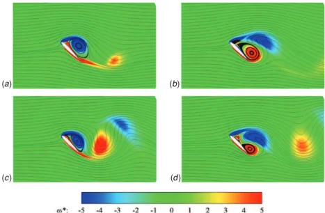
Figure 2 displays the non-dimensional vorticity flow fields relative to the first test case. Figure3 shows a comparison

(a)

(c)

(b)

(d)

Figure 2.Non-dimensional spanwise vorticity flow fields and stream lines at times t∗_{= 2 (a), 4 (b), 6 (c) and 8 (d).}

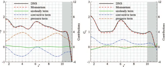
Figure 3.Comparison between the coefficients obtained by integrating the pressure and the viscous stresses along the airfoil surface (DNS) and by applying the momentum equation (momentum) to the 2D velocity fields—first test case.

Table 1.Mean values of the drag and lift coefficients and their respective unsteady, convective and pressure contributions computed with different spatio-temporal resolutions and introduction of random noise.

CD Unst. Conv. Press. CL Unst. Conv. Press.

Ref. (600 × 600) 1.396 0.077 −1.402 2.721 1.256 −0.074 1.332 −0.003 400 × 400 1.390 0.077 −1.394 2.707 1.254 −0.072 1.328 −0.002 200 × 200 1.372 0.073 −1.471 2.770 1.213 −0.072 1.304 −0.019 Noise 1t∗_{= 0.12 1.400 0.077 −1.404 2.728 1.258 −0.073 1.333 −0.002} Noise 1t∗_{= 0.35 1.398 0.077 −1.404 2.726 1.257 −0.073 1.333 −0.003} Noise 1t∗_{= 1.40 1.502 0.144 −1.404 2.762 1.315 −0.008 1.333 −0.010}

between the unsteady lift and drag coefficients CL and CD obtained by means of the momentum equation and by

integrating the pressure and the viscous stresses along the airfoil surface. For a better comprehension, the corresponding unsteady, convective and pressure contributions are added. The comparison reveals that both lift and drag estimations are correct despite slight discrepancies probably arising from discretization errors and grid interpolation step. The mean

values of the respective contributions are computed over the interval t∗ = [1; 10] and given in table 1 so as to facilitate comparisons with the lift and drag obtained using flow fields subjected to a lower spatial resolution or to a random noise. The mean absolute errors computed for such varying parameters are listed in table2.

Two simple remarks are addressed: the unsteady term exhibits weak amplitude oscillations around zero (by

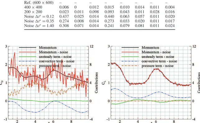
Table 2.Mean absolute errors (relative to reference case) committed on the drag and lift coefficients and their respective unsteady, convective and pressure contributions computed with different spatio-temporal resolutions and introduction of random noise.

CD Unst. Conv. Press. CL Unst. Conv. Press.

Ref. (600 × 600) – – – – – – – – 400 × 400 0.006 0 0.012 0.015 0.010 0.014 0.011 0.004 200 × 200 0.023 0.011 0.098 0.093 0.043 0.011 0.028 0.016 Noise 1t∗= 0.12 0.437 0.025 0.014 0.440 0.063 0.057 0.011 0.020 Noise 1t∗= 0.35 0.274 0.008 0.014 0.273 0.033 0.020 0.011 0.017 Noise 1t∗= 1.40 0.308 0.071 0.014 0.241 0.079 0.081 0.011 0.024

Figure 4.Influence of a 2.5% uniformly distributed random noise on the deduction of drag (left) and lift (right) and their respective unsteady, convective and pressure contributions with 1t∗_{set to 0.35.}

definition, its mean value tends to zero); the pressure term relative to the lift evaluation is negligible. The latter arises from the fact that the upper and lower limits of the control volume, from which the pressure contribution to lift is integrated, are not subjected to steep velocity and pressure gradients. As we will see in the following sections, both observations are favourable to the consistency of the experimental loads prediction as it minimizes the difficulties linked to (1) the temporal resolution and (2) the pressure evaluation.

3.2. Spatial resolution

In order to evaluate the influence of the spatial resolution on the forces obtained by the momentum balance, the previous calculation is reiterated for Cartesian grids of lower resolution (400 × 400 and 200 × 200 cells, the resolution of the reference case being 600 × 600 for a 10 × 10 c2_{field). In table2, the}

mean absolute errors (over the interval t∗_{= [1; 10]) introduced}

on the different contributions are given. It is shown that the convective and pressure terms relative to the drag prediction are affected in a stronger way than those relative to the lift prediction. Respectively, for the lower resolution (200 × 200), the mean absolute errors are 0.098, 0.093 and 0.028, 0.016. This remark is attributable to the fact that the zones of integration for the convective and pressure terms relative to the lift (upper and lower limits of the control volume) are far away from the wake and consequently not very prone to

the velocity and pressure gradients. In addition, it is noticed that the resolution has little influence on the unsteady term, the error related to it being minimized by the dimensions of the integration domain (integration on the control volume and not the surface). Note that these deviations compensate for each other in the case of drag prediction, leading to a weak mean absolute error of 0.023.

3.3. Velocity noise

The velocity vectors determined by DNS are here disturbed by a random error. Considering the spatial resolution used in both numerical and experimental data, a uniform distribution leading to a mean absolute uncertainty of 0.1 pixel (as commonly measured in PIV experiments, e.g. Stanislas

et al2005) is introduced in order to assess the influence of experimental errors on the evaluation of lift and drag. Note that, with respect to the airfoil translational speed, 0.1 pixel corresponds to a relative error of 2.5%.

Figure 4 illustrates the influence of noise on the drag and lift predictions and their respective contributions. On the one hand, it is shown that the introduction of a random error significantly affects the drag component. This effect comes from the fact that the pressure term, whose contribution is here substantial, is strongly degraded due to (1) the presence of differential operators in equation (2) which tend to amplify the measurement error and (2) the phenomenon of error propagation discussed in section2. Conversely, the unsteady

Figure 5.Mean values and mean absolute errors of the drag coefficient and its contributions as a function of 1t∗_.

and convective terms are quasi-insensitive to the presence of noise. One can note from equation (1) that their analytical formulations require respectively no and only one derivation step. Results in table 2 demonstrate that the mean error committed on the pressure term accounts for roughly all of the total mean absolute error committed on the drag component. On the other hand, the lift evaluation appears more robust to the presence of noise. As previously put into evidence, both unsteady and convective terms are quasi-unaffected. Furthermore, the instantaneous contribution of the pressure term does not exceed 2% of the lift component. Hence, the mean error committed on the latter is nearly equally shared among the unsteady, convective and pressure terms. For an adequate value of 1t∗ (see the following section), the introduction of a 2.5% uniformly distributed random noise leads to a mean error of respectively 15.6% and 1.6% on the drag and lift predictions.

3.4. Temporal resolution

If the error relative to the introduction of a random noise is directly transmitted to the convective term of equation (1), its influence on the unsteady and pressure terms indirectly depends on the value of 1t used in equations (1) and (2). Theoretically, an increase of 1t tends to minimize the parasitic temporal variations induced by the presence of noise but, in parallel, causes a loss of information on the intensity of the acceleration fields. Figure5plots the mean values and mean absolute errors of the drag coefficient and its contributions as a function of 1t∗. Specific values are listed in table 2. The results demonstrate that increasing the time step from 1t∗ = 0.12 to 1t∗ _{= 0.35 decreases the mean absolute error}

committed on the unsteady and pressure terms relative to the drag evaluation by respectively 68% and 38%, without affecting their mean values. Analogous effects are put into evidence for the unsteady and pressure terms relative to the lift evaluation with a reduction of respectively 65% and 15%. This improvement is optimum on the interval [0.5; 1], after which the loads evaluation is degraded. It is shown that further increasing the time step to 1t∗= 1.40 leads to a wrong

evaluation of the acceleration. As a result, the mean lift and drag are overestimated by respectively 4.7% and 7.6%. This overestimation does not seem critical though; the contributions of the unsteady term and the unsteady part of the pressure term being weak for both lift and drag components.

For this first test case, fixing 1t∗ to approximately 0.5 appears to be a suitable parameterization. The theoretical analysis of the stability behind a NACA0012 airfoil (Dergham

et al2009) brings St = fcsin(α)/V0 = 0.124, where St is the

non-dimensional vortex shedding frequency f and α is the angle of attack. According to this value, a sufficient temporal resolution is obtained by discretizing the characteristic time scale of the flow in approximately 10 instants, which is surprisingly low.

3.5. Spanwise component

The experimental reproduction of two-dimensional configurations is particularly delicate due to the influence of the boundary conditions (e.g. end plates) which may imply the presence of a three-dimensional velocity component. In other words, the velocity flow fields obtained by PIV2D-2C may not be strictly free of divergence. Thus, the aim of this section is to evaluate the influence of such a 3D component on the determination of loads by means of the momentum equation approach. The second test case is here considered. The momentum equation approach is applied to the planar velocity flow fields obtained at mid-span λ/2. The resulting aerodynamic loads are compared to those deduced from the integration of the pressure and the viscous stresses along the airfoil surface in the same plane (figure6).

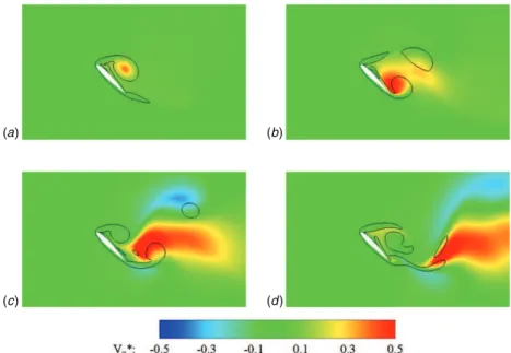
In contrast to the lift coefficients, it is shown that the unsteady behaviour of the drag coefficients significantly differs from t∗ = 2. The representation of the third velocity component contours (figure7) suggests that there might be a link between this offset and the interaction spanwise velocity regions/control volume limits. Some specifications may be addressed. First, physical features exhibiting substantial spanwise velocities do not interact with the upper and lower limits of the control volume. Consequently, the

Figure 6.Comparison between the coefficients obtained by integrating the pressure and the viscous stresses along the airfoil surface (DNS) and by applying the momentum equation (momentum) to the 2D velocity fields at mid-span—second test case.

(a)

(c)

(b)

(d)

Figure 7.Non-dimensional spanwise velocity flow fields and iso-vorticity magnitude contour |ω∗| = 4 in the mid-span plane at times t∗_{= 2}

(a), 4 (b), 6 (c) and 8 (d).

convective and pressure terms relative to the lift coefficient are not significantly affected. Furthermore, considering the conformity between momentum and DNS lift coefficients, the presence of a third component does not seem to significantly alter the unsteady term. In contrast, spanwise velocity structures continually cross the downstream limit of the control volume from t∗= 2. The convective and pressure terms relative to the drag coefficient are hence significantly affected. The resulting error committed on the latter may reach 50% for spanwise velocities of the order of 0.5 V0. Such observations

suggest that, besides the obviousness that a two-dimensional approach is not adapted to three-dimensional flows, a coherent lift force may still be obtained if a suitable control volume is used. Furthermore, one may have a quantitative estimation of

the accuracy of the results if the magnitude of the spanwise component is known.

3.6. Inertial component

When non-constant motion laws are prescribed, an inertial contribution arises from the added mass or virtual mass effects. In order to ensure that the latter is correctly taken into account, the momentum balance is applied to the third test case. Note that the inertial contribution is simply deduced from the knowledge of the airfoil boundary conditions and is contained in the convective term of equation (1). Figure 8 compares the unsteady lift and drag coefficients obtained by means of the momentum equation and by integrating the pressure and the viscous stresses along the airfoil surface. For the sake of

Figure 8.Comparison between the coefficients obtained by integrating the pressure and the viscous stresses along the airfoil surface (DNS) and by applying the momentum equation (momentum) to the 2D velocity fields—third test case.

clarity, the inertial part (after 10 t∗) is darkened. Note that the rotation of the airfoil induces a lift bump through the Kramer effect. The latter is followed by a sharp decrease of both lift and drag due to the airfoil deceleration.

4. Application on experimental data

Although the momentum balance theory appears relatively simple, its application on experimental data is delicate as submitted to experimental uncertainties, principally affecting the deduction of the pressure along the control surface. However, the approach is particularly convenient when considering low Reynolds flows or moving bodies which limit the use of gauges. Here, the momentum equation is applied to the experimental flow fields measured by TR-PIV on a 2D NACA0012 airfoil at Reynolds 1000. Specifically, we focus on the flow generated by the impulsive start of the airfoil at high angle of attack, as described in section3. The correlation between vorticity flow fields and aerodynamic coefficients is addressed.

4.1. Experimental set-up

The instruments and procedures used in the experiments have been described elsewhere (Jardin et al2009). A transparent NACA0012 profile of chord 60 mm and span 50 cm, placed between two end plates in a 1 × 1 × 2 m3 _{water tank, is}

translated by means of a servo-controlled motor. TR-PIV measurements are performed on the spanwise symmetry plane using two JAI 8-bits cameras placed side by side. The laser sheet is provided by a continuous argon laser system. Thirty per cent of the laser illuminates one side of the profile while 70% is transported through an optical fibre to illuminate the other side. Such an experimental set-up allows access to all regions of the flow that might have been hidden by perspective or shadow effects. This aspect appears as essential when dealing with the momentum equation approach. The two-dimensional velocity flow fields are deduced every 1t∗ ₌

0.014 (where 1t∗ is the non-dimensional time step between

two images used for the cross correlation) using a multipass algorithm with a final interrogation window size of 16 × 16 pixels (LaVision software). The 2% spurious velocities are identified and replaced using both peak ratio and median filters. The NACA0012 airfoil is impulsively started at a constant speed V0= 1.67 cm s−1and with a fixed angle of attack α0=

45◦. The pure translational motion is maintained throughout 6 chords, corresponding to an adimensional travel time of 6 t∗. Here, the inertial effects arising from the mechanical set-up and motors may be considered negligible.

4.2. Parameters setting

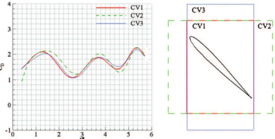
Theoretically, the aero-hydrodynamic loads determined by means of the momentum equation approach are insensitive to the dimensions and size of the control volume. Practically, its definition requires attention as it directly affects the relative contributions of the unsteady, convective and pressure terms. Keeping in mind that the evaluation of the pressure around the control volume is subjected to some difficulties, it is here convenient to use a control volume which minimizes both the contribution of the pressure term and the error propagation phenomenon. For the lift evaluation, the first condition is ensured by placing the upper and lower limits away from the wake, i.e. away from steep velocity and pressure gradients regions (e.g. CV3 in figure 9). For the drag evaluation, the downstream limit being subjected to significant gradients in all cases, a relatively small domain is used in order to lower the effect of error propagation (e.g. CV1 in figure9). Figure 9 shows the influence of the control volume on the deduction of the instantaneous drag coefficient generated by the impulsive start of a NACA0012 airfoil at Reynolds 1000. The corresponding control volumes are displayed.

Moreover, in accordance with the previous analysis carried out on the temporal resolution, figure10shows that the dispersion is significantly weakened with increasing time step 1t∗. Consequently, its value is fixed to 1t∗_{= 0.68, i.e. above}

the threshold value of 0.5 defined in section3. A polynomial fitting function is then defined, based on the corresponding

Figure 9.Influence of the control volume on the drag evaluation.

Figure 10.Experimental unsteady drag (left) and lift (right) coefficients calculated with different time steps.

results. Besides, as reported earlier, one can note that the typical dispersion of the drag is significantly stronger than that of lift.

4.3. Flow dynamics/loads correlation

In this section, we put into evidence the correlation between the vorticity flow fields (figure 11) and the resulting lift and drag coefficients (figure 12) obtained experimentally on an impulsively started NACA0012 airfoil at Reynolds 1000.

The motion starts at t∗= 0. Due to the high angle of attack, the flow instantly stalls at the leading edge, forming the so-called leading edge vortex or LEV (blue vorticity in figure11). In parallel, one can clearly observe the formation of the starting vortex, denoted as a red vorticity spot in the vicinity of the airfoil trailing edge. The circulation establishment is here quasi-immediate, the Wagner effect being negligible at such Reynolds numbers. The production of vorticity at the leading edge is continuously fostered by the translation, resulting in the formation of a low-pressure suction region on the upper surface of the airfoil. Hence, both lift and drag rapidly reach substantial levels. The latter is maintained between t∗ = 0

and t∗ ≈ 1.5, corresponding to the close attachment of the LEV. Nevertheless, after t∗ ≈ 1.5, the further accumulation of vorticity, combined with the action of the trailing edge vortex (TEV) formation, leads to the LEV instability. As a consequence, the latter is progressively shed into the wake, resulting in a sharp decrease of both lift and drag. The drag exhibits a local minimum near t∗ ≈ 2.6, followed by a bump at t∗ ≈ 3.7 deriving from the formation of the TEV. In contrast, the latter does not significantly affect the lift whose local minimum is thus reached near t∗≈ 3.2. As the first LEV is convected downstream, a second LEV is formed alternatively with the previous TEV, inducing the so-called von Karman street. The presence of this second LEV on the airfoil upper surface sustains the production of lift and drag whose coefficients reach another local maximum at t∗≈ 5.4. Afterwards, the loads decrease again, leading to a periodic shedding state which cannot be put into evidence in this study since the translation length is limited to 6 chords. One important feature here is that substantial levels of lift and drag are reached during a longer period at the onset of the motion. This phenomenon, also referred to as the dynamic stall mechanism, is a common feature in rotating blades and flapping wings aerodynamics.

(c) (b) (a)

Figure 11.Non-dimensional experimental vorticity flow fields and stream lines resulting from the impulsive start of a NACA0012 airfoil at t∗_{= 2 (a), 4 (b) and 6 (c) from top to bottom.}

Therefore, it is demonstrated that the temporal behaviour of the loads matches the spatio-temporal evolution of the vortical structures. In the range t∗ = 1–6, typical levels of

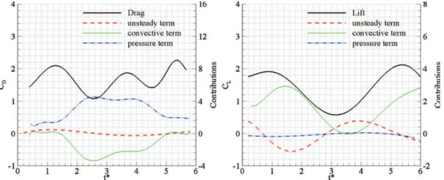
Figure 12.Experimental drag (left) and lift (right) coefficients and their respective unsteady, convective and pressure contributions resulting from the impulsive start of a NACA0012 airfoil—filtered data.

Figure 13.Experimental unsteady, convective and pressure contributions of the drag coefficient resulting from the impulsive start of a NACA0012 airfoil—raw data.

lift and drag corresponding to the development of vortical structures in the vicinity of the airfoil are comparable in both experimental and numerical cases. However, some discrepancies exist. First, we can observe a time offset attributable to a delay in the formation and development of vortical structures. Second, differences in amplitudes deriving from both experimental errors and numerical diffusivity are noticed. Focusing on the influence of experimental errors, it is here convenient to display the unsteady, convective and pressure contributions of the lift and drag components. It is shown that relatively strong differences between experimental and numerical results are put into evidence when the pressure contribution is preponderant, as illustrated by the surprising levels reached by the drag near t∗ = 3.7, i.e. due to the formation of the TEV. In addition, the presence of spurious vectors at this specific instant may affect the measurement accuracy and further alter the results. Figure 13 confirms that this instant is critical and suggests that, throughout the whole motion, the main dispersion comes from the unsteady

and pressure term, as previously described in section3. In contrast, in accordance with the numerical tests, the pressure contribution of the lift coefficient is negligible, making its evaluation more robust.

5. Conclusion

Measuring the loads experienced by an airfoil through the momentum equation approach appears a powerful method for several reasons. Besides the fact that the approach is non-intrusive as applied on TR-PIV velocity flow fields, it is particularly convenient for low Reynolds flows or for moving airfoil configurations (as encountered for flapping wing MAVs applications), whose resulting forces have strong uncertainties due either to their weak values or to the influence of an inertial component. Moreover, it allows an accurate temporal correlation between the loads and the vortex structures, hence giving further insight into the force generating mechanisms.

First, the present work evaluates the influence of the different parameters specific to the calculation of the momentum equation and validates the method using DNS velocity flow fields around an impulsively started 2D NACA0012 airfoil at Reynolds 1000. It is found that the spatial resolution principally affects the convective and pressure contributions to drag since the limits of integration relative to their calculation are subjected to steep velocity and pressure gradients. Nevertheless, its global influence on the resulting force is weak; the discrepancy between the reference case and the lower resolution case does not exceed 5%. Furthermore, the introduction of a 2.5% random noise demonstrates that the principal errors attributable to the measurement uncertainties derive from the pressure term. This effect is due to the use of differential operators and, to a minor extent, the phenomenon of error propagation. Consequent to this remark, the lift evaluation appears more robust to the presence of noise than the drag evaluation, the contribution of the pressure term being negligible in this case. In addition, it is worth highlighting that the error induced by a random noise highly depends on the time step used to compute the acceleration fields. For an adequate value of this time step, the mean errors committed on the drag and lift coefficients are respectively 15.6% and 1.6%. The analysis of the influence of the temporal resolution surprisingly suggests that discretizing the characteristic time scale in 10 instants is sufficient to accurately describe the flow dynamics. Besides, it is shown that the two-dimensional approximation of the momentum equation approach is not valid when applied to three-dimensional flows. This observation is notably verified when the positions of spanwise velocity regions coincide with the positions of the integration limits.

Second, the momentum balance is applied to experimental TR-PIV velocity flow fields. A similar configuration as previously considered for the parametrical study is

analysed. Despite discrepancies resulting from experimental uncertainties and a time delay denoted between both experimental and numerical approaches, the resulting lift and drag demonstrate a clear correlation with the spatio-temporal behaviour of the vortical structures. Moreover, the influence of their respective unsteady, convective and pressure contributions augments the previous conclusions on numerical data.

Future work will concentrate on adapting the momentum equation method to three-dimensional flows.

References

Dergham G, Sipp D and Jacquin L 2009 On the frequency selection for two-dimensional thin and bluff body wakes Phys. Fluids submitted

Jardin T, David L and Farcy A 2009 Characterization of vortical structures and loads based on time-resolved PIV for asymmetric hovering flapping flight Exp. Fluids

46847–57

Jones B M 1936 Measurement of profile drag by the pitot-traverse method ARC R&M 1688

Kat R, Van Oudheusden B W and Scarano F 2008 Instantaneous planar pressure field determination around a square-section cylinder based on time-resolved stereo-PIV 14th Symp. App.

Las. Tech. Fluid Mech. (Lisbon, Portugal)

Kurtulus D F, David L, Farcy A and Alemdaroglu N 2008 Aerodynamic characteristics of flapping motion in hover Exp.

Fluids4423–36

Kurtulus D F, Scarano F and David L 2007 Unsteady aerodynamic forces estimation on a square cylinder by TR-PIV Exp. Fluids

42186–96

Lighthill J 1986 Fundamentals concerning wave loading on offshore structures J. Fluid Mech.173667–81

Lin J C and Rockwell D 1996 Force identification by vorticity fields: techniques based on flow imaging J. Fluids Struct.10663–8

Moreau J J 1952a Bilan dynamique d’un ´ecoulement rotationnel

J. Math. Pures Appl. 31355–75

Moreau J J 1952b Bilan dynamique d’un ´ecoulement rotationnel

J. Math. Pures Appl. 321–78

Noca F, Shiels D and Jeon D 1997 Measuring instantaneous fluid dynamic forces on bodies, using only velocity fields and their derivatives J. Fluids Struct.11345–50

Noca F, Shiels D and Jeon D 1999 A comparison of methods for evaluating time-dependent fluid dynamic forces on bodies, using only velocity fields and their derivatives J. Fluids Struct.

13551–78

Protas B, Styczek A and Nowakowski A 2000 An effective approach to computation of forces in viscous incompressible flows

J. Comput. Phys.159231–45

Quartapelle L and Napolitano M 1982 Force and moment in incompressible flows AIAA J.21911–3

Stanislas M, Okamoto K, K¨ahler C J and Westerweel J 2005 Main results of the second international PIV challenge Exp. Fluids

39170–91

Unal M F, Lin J C and Rockwell D 1997 Force prediction by PIV imaging: a momentum based approach J. Fluids Struct.

11965–71

Van Oudheusden B W, Scarano F and Casimiri E W F 2006 Non-intrusive load characterization of an airfoil using PIV Exp.