Sensitivity and optimal forcing response in separated boundary layer flows

Science Arts & Métiers (SAM)

is an open access repository that collects the work of Arts et Métiers Institute of

Technology researchers and makes it freely available over the web where possible.

This is an author-deposited version published in: https://sam.ensam.eu

Handle ID: .http://hdl.handle.net/10985/6862

To cite this version :

Frédéric ALIZARD, Stefania CHERUBINI, Jean-Christophe ROBINET - Sensitivity and optimal forcing response in separated boundary layer flows Physics of Fluids Vol. 21, n°064108, p.3 -2009

Any correspondence concerning this service should be sent to the repository

Frédéric Alizard, Stefania Cherubini, and Jean-Christophe Robinet

Citation: Phys. Fluids 21, 064108 (2009); doi: 10.1063/1.3153908 View online: http://dx.doi.org/10.1063/1.3153908

View Table of Contents: http://pof.aip.org/resource/1/PHFLE6/v21/i6 Published by the American Institute of Physics.

Related Articles

Instability of a backward-facing step flow modified by stationary streaky structures Phys. Fluids 24, 104104 (2012)

Dynamics of magnetic chains in a shear flow under the influence of a uniform magnetic field Phys. Fluids 24, 042001 (2012)

Boundary layer development in the flow field between a rotating and a stationary disk Phys. Fluids 24, 033601 (2012)

Slip boundary for fluid flow at rough solid surfaces Appl. Phys. Lett. 100, 074102 (2012)

Wang’s shrinking cylinder problem with suction near a stagnation point Phys. Fluids 23, 083102 (2011)

Additional information on Phys. Fluids

Journal Information: http://pof.aip.org/about/about_the_journal Top downloads: http://pof.aip.org/features/most_downloaded Information for Authors: http://pof.aip.org/authors

Sensitivity and optimal forcing response in separated boundary layer flows

SINUMEF Laboratory, Arts and Métiers, ParisTech, 151 Bd. de l’Hôpital, 75013 Paris, France

共Received 16 June 2008; accepted 8 May 2009; published online 26 June 2009兲

The optimal asymptotic response to time harmonic forcing of a convectively unstable two-dimensional separated boundary layer on a flat plate is numerically revisited from a global point of view. By expanding the flow disturbance variables and the forcing term as a summation of temporal modes, the linear convective instability mechanism associated with the response leading to the maximum gain in energy is theoretically investigated. Such a response is driven by a pseudoresonance of temporal modes due to the non-normality of the underlying linearized evolution operator. In particular, the considered expansion on a limited number of modes is found able to accurately simulate the linear instability mechanism, as suggested by a comparison between the global linear stability analysis and a linearized direct numerical simulation. Furthermore, the dependence of such a mechanism on the Reynolds number and the adverse pressure gradient is investigated, outlining a physical description of the destabilization of the flow induced by the rolling up of the shear layer. Therefore, the convective character of the problem suggests that the considered flat plate separated flows may act as a selective noise amplifier. In order to verify such a possibility, the responses of the flow to the optimal forcing and to a small level of noise are compared, and their connection to the onset of self-excited vortices observed in literature is investigated. For that purpose, a nonlinear direct numerical simulation is performed, which is initialized by a random noise superposed to the base flow at the inflow boundary points. The band of excited frequencies as well as the associated peak match with the ones computed by the asymptotic global analysis. Finally, the connection between the onset of unsteadiness and the optimal response is further supported by a comparison between the optimal circular frequency and a typical Strouhal number predicted by numerical simulations of previous authors in similar cases. © 2009 American Institute of Physics. 关DOI:10.1063/1.3153908兴

I. INTRODUCTION

When a laminar boundary layer encounters a sufficiently large adverse pressure gradient, a laminar separation bubble 共referenced as LSB hereafter兲 occurs. Many engineering ap-plications such as low Reynolds number aerodynamics con-figurations of airfoils or car industries and turbomachineries involve typical structures of LSB. Since the first observations of Jones,1 flow separation was extensively studied, experi-mentally as well as numerically. A part of these prior re-searches deals with its time-averaged mean and steady struc-ture such as the experimental work of Gaster,2 the first numerical attempt of Briley,3 and the method of matched asymptotic expansions provided by the triple deck theory.4

A typical feature of LSB is its very unstable nature and its high sensitivity to background disturbances, even at low Reynolds numbers. This property is often synonymous of loss of aerodynamic performances such as increase in the drag or loss of lift on airfoils at angle of attack close to static stall values. As a consequence, many investigations have been carried out on the onset of unsteadiness in several con-figurations; for instance, the flat plate separated boundary layer has been studied by means of direct numerical simula-tions共referenced as DNSs hereafter兲5,6and experiments,7as

well as the backward facing step flow共see Refs.8and9for instance兲. In particular, the self-sustained oscillatory behav-ior as well as the role of topological changes in the separated flows has received a lot of attention during the last two de-cades. More specifically, it is now well established that the onset of global instabilities observed in absence of perma-nent external perturbations is related to the existence of a local absolute instability.10 In that respect, the nonlinear se-lection criteria based on local properties of the flow used by Marquillie and Ehrenstein11was allowed to explain the glo-bal high frequency unsteadiness of a recirculation bubble confined between two bumps. This global instability mecha-nism is characterized by a resonator dynamics similar to the one observed in many open shear flows, for instance, the self-sustained oscillations occurring in the wake of a cylinder.12In such cases, the associated space-time dynamics of the flow is intimately connected to the existence of an unstable global mode. A resonator dynamics driven by a three-dimensional mechanism was observed in a flat plate separated flow by Theofilis et al.,13 in a flow over a back-ward facing step by Barkley et al.14 or behind a bump by Gallaire et al.15The same authors identified a slowly ampli-fied, large scale, stationary, and unstable global mode, not revealed by a local instability analysis, which is able to in-duce a topological change in the flow.

Nevertheless, some authors recently conjectured that the occurrence of self-sustained oscillations in separated flows

a兲_{Author to whom correspondence should be addressed. Electronic mail:} frederic.alizard@paris.ensam.fr.

b兲_{Also at DIMEG, Politecnico di Bari, Via Re David 200, 70125 Bari, Italy.}

PHYSICS OF FLUIDS 21, 064108共2009兲

observed numerically or experimentally may be attributed not only to a resonator dynamics, but should also take into account the influence of external perturbations, as discretiza-tion errors in numerical simuladiscretiza-tions or environment noise occurring in experiments. For instance, Kaiktsis et al.9 re-ported discrepancies among various numerical simulations of the time asymptotic state of a two-dimensional 共2D兲 flow over a backward facing step. Typically, the onset of global unsteadiness appears to be closely dependent on the numeri-cal method and the grid resolution and well below the emer-gence of an unstable global mode, as reported by Barkley et al.14The response of the convective modes to the level of background noise due to the discretization errors is thus pro-posed by Kaiktsis et al.9to explain such discrepancies in the asymptotic regime. A similar convective mechanism sus-tained by the presence of numerical noise is proposed by Wasistho et al.16 as an explanation of the onset of unsteadi-ness in a flat plate separated flow. All these studies suggest that an inherent random background noise may generate un-steadiness in a separated flow. Therefore, the amplifier char-acter of the flow which is due to the presence of a convec-tively unstable region may play a major role in the capability of the flow to self-sustain perturbations. Nevertheless, the onset of unsteadiness and selected frequencies are still an open question at which no clear answer is as far as we know provided.

In the present contribution, we reassess the selective noise amplifier dynamics of a typical flat plate separated flow by means of a so-called global linear stability approach based on 2D temporal eigenmodes.17 In particular, the con-vective instability mechanism underlying the global optimal response to a harmonic forcing and its associated energy gain in the asymptotic regime is investigated. It is worth to notice that such a methodology is relevant in the configuration here considered, where nonparallel effects are not negligible. Since the seminal work of Cossu and Chomaz1810 years ago on the space-time dynamics of open flows, and the review of Chomaz19 in 2005, it is well known that a global amplifier dynamics could derive from the convective instabilities due to the nonorthogonality of the set of global eigenmodes as-sociated with the considered flow. Since then, this topic has received the attention of several researchers, turning into a vivid research field. In particular, in the previous works of Ehrenstein and Gallaire,20Alizard and Robinet,21and Åker-vik et al.22 on a flat plate boundary layer, a large transient growth has been observed due to the optimal nonmodal am-plification of a localized perturbation. An appropriate super-position of global eigenmodes has shown that the optimal perturbation takes the form of a wave packet traveling along the flat plate and amplifying itself, leading to an increase in the kinetic energy of the perturbation.

Furthermore, similar global stability analysis have been performed in various configurations as a falling liquid cur-tain by Schmid and Henningson,23 an open cavity flow by Åkervik et al.24 and Henningson and Åkervik,25 or a flow behind a bump by Ehrenstein and Gallaire26and pointed out new physical understandings on the low-frequency global unsteadiness of open flows as the flapping effect occurring in separation bubbles,7 which was explained in terms of an

in-teraction of modes. The regeneration of the wave packet traveling along the flow under the influence of a convective mechanism leads to a low-frequency beating.

Furthermore, Blackburn et al.27 and Marquet et al.28 studied the convective instability mechanism emerging in separated flow over a step by means of an optimization strat-egy involving the integration in time of the direct and adjoint linearized Navier–Stokes equations. The results obtained by such a method, called “direct optimal growth analysis” by Blackburn et al.,27 confirmed the large transient growth re-sulting from the convective amplification of a wave packet localized in space. Such studies have thus provided a first attempt to relate the unsteadiness observed in numerical simulation and laboratory experiments in the considered flows with the noise amplifier dynamics derived from the optimal transient behavior.

It is worth to point out that all these studies present common features which rely on the non-normality of the governing linear operator, as noticed in Ref.29. Neverthe-less, none of them are dedicated to a specific investigation of the global response to an external forcing and its relationship with the onset of unsteadiness in the asymptotic regime, un-der the assumption of a permanent residual noise. Conse-quently, it seems interesting to develop a strategy based on the non-normality of temporal modes similar to the one in Refs. 20–22 in order to describe the optimal response to a harmonic forcing in the considered flow, which could result in a selective noise amplifier dynamics somewhat connected to the onset of unsteadiness observed in DNSs of separated flows by Wasistho et al.,16 Pauley et al.,30 and Ripley and Pauley.31

The present work, which deals with 2D globally stable flat plate separated flows, focuses on the description of the convective mechanism underlying the optimal response and investigates the effect of the high sensitivity to external forc-ing on the destabilizforc-ing physics in the asymptotic regime. The paper is organized as follows. In Sec. II a brief descrip-tion is given of the numerical tools employed for the com-putation of the base flow.

In Sec. III, an analysis of the non-normality of the tem-poral evolution operator is provided by the computation of pseudospectra. Such an analysis is found to be able to de-scribe the triggering of convective waves in the asymptotic regime through a pseudoresonance of the temporal modes. A specific study of the resolvent norm is carried out in order to identify the most responsive disturbance and the underlying amplification mechanism. The reduced model derived from the 2D temporal modes summation is then validated by per-forming a comparison with a linearized DNS. Later, an in-vestigation is carried out on the effects of the increase in the adverse pressure gradient and/or the Reynolds number on the resolvent norm as well as on the spatial distribution of the associated most responsive disturbance. Such results are able to bring new elements on the influence of the shear layer on the instability mechanism.

Finally, nonlinear numerical simulations are performed initialized by the considered flow perturbed randomly at the inlet points, in order to find a connection between the selec-tive noise amplifier behavior derived from the optimal

re-sponse to harmonic forcing and the onset of unsteadiness observed in separated flows. Therefore, a possible scenario is proposed related to the onset of unsteadiness in a flat plate separated flow, which is supported by the results of the present analysis and by a comparison with literature.

II. BASIC STATES A. Some generalities

The incompressible 2D Navier–Stokes equations are written in the vorticity-stream function共W,⌿兲 formulation,

⳵W ⳵t + U ⳵W ⳵x + V ⳵W ⳵y = 1 Re

冉

冊

冉

冊

where Re represents the Reynolds number and 共U,V兲 the

velocity fields as U =⳵⌿/⳵y and V = −⳵⌿/⳵x.

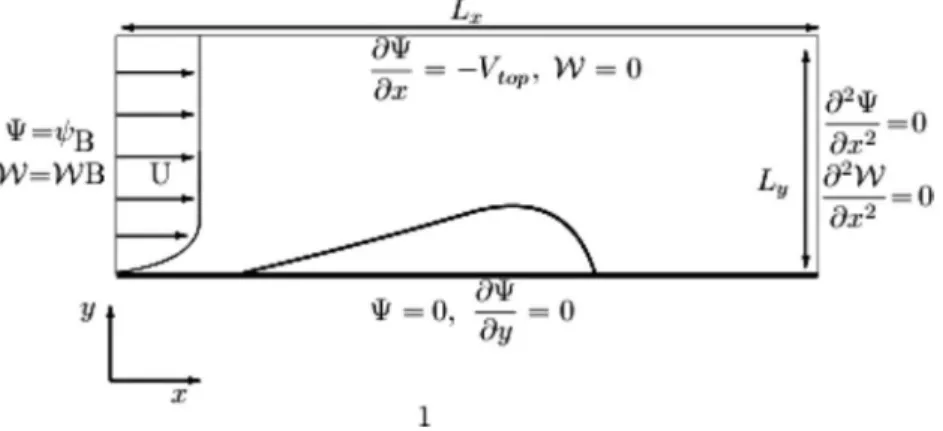
In order to induce a well defined separated zone, a spe-cific suction profile at the upper boundary points is pre-scribed. A Blasius profile at the inflow, referenced asWB,⌿B outflow and wall boundary conditions complete system共1兲 as depicted in Fig.1.

B. Numerical method

The time discretization of Eq.共1兲 is performed using a

second order Adams–Bashforth/backward-differentiation

scheme based on an implicit treatment of the viscous terms and an explicit treatment of the advection terms,

1 ⌬t

冉

冊

冉

冊

The vorticity as well as the stream function are dis-cretized using a spectral collocation method based on Cheby-shev polynomials in the wall normal direction and a second order finite difference scheme in the streamwise direction. The most difficult task in the discretization of the

vorticity-stream function formulation is the definition of the vorticity at the wall where no explicit boundary condition is known. In order to provide an accurate implementation of the no-slip condition, an influence matrix method is used to compute the vorticity at the wall. A similar approach was used by Daube32 in a vorticity-velocity formulation. This technique allows to verify exactly the Neumann boundary condition of the stream function. The methodology is detailed by Peyret33 which further illustrates the numerical matters.

Consequently, at each time step four linear systems have to be solved and a matrix productM−1_{S, giving the vorticity} values at the wall, is performed. The matrixM is the influ-ence matrix whereas S is computed from the Neumann con-dition applied at boundary points on the stream function, and is updated at each time step. The build ofM as well as its inversion are realized in the preprocessing stage. The spec-tral discretization in the wall normal direction coupled with the influence matrix technique allows to obtain an accurate definition of the no-slip boundary condition at the wall. Fi-nally, a direct method based on a Thomas algorithm is used to solve the implicit system as well as the Poisson equation, taking into account the block tridiagonal matrix structure.

The DNS allows to approach a steady state solution. A Newton procedure based on the library NITSOL 共Ref. 34兲

achieves the convergence of the base flow by means of a continuation procedure.

C. Flat plate separated flows

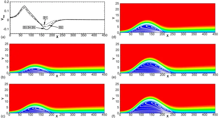
Five base flows, characterized by a different suction pro-file and/or Reynolds number, are computed and depicted in Figs.2共b兲–2共f兲. The Reynolds number Re_␦based on the dis-placement thickness at x = 0 varies from 200 to 220 which is below the critical Reynolds number for convective instabili-ties. The dimensions of the computational box are Lx= 525 and Ly= 25. A共1000⫻100兲 point grid allows to obtain a well converged base flow. Furthermore, such a grid is regular in the streamwise direction and clustered near the wall in the normal direction by means of a classical transformation from a Gauss–Lobatto grid.

The base flows labeled from D1 to D3 are computed at a Reynolds number Re_␦= 200 for the three suction profiles dis-played in Fig.2共a兲. The separated flows D4 and D5 are ob-tained by using the same upper boundary velocity distribu-tion as D3, for the Reynolds numbers Re_␦= 215 and Re_␦

FIG. 1. Computational box and boundary conditions associated with the base flow.

= 220, respectively. One may observe in Figs.2共b兲–2共f兲 the influence of these parameters on the resulting base flows. An increasing intensity of the suction implies a larger separated zone as well as a displacement of the center of the bubble near the reattachment point. A slight increase in the Reynolds number value causes an increase in the bubble size and of the recirculation close to the reattachment point. Moreover, un-der the same adverse pressure gradient, the location of the separation point is only slightly affected by the increasing of Re_␦共TableI兲. The stability of such base flows is analyzed in

the next sections with the aim of determining the influence of the shape of the bubble on the spatial distribution of the most responsive disturbance.

III. CONVECTIVE INSTABILITY ANALYSIS: A SELECTIVE NOISE AMPLIFIER

A. Global linear stability: Some theory and problem definition

In this section the base flow variables are denoted by •¯. We investigate the evolution in space and time of a small perturbation superposed to a 2D flat plate separated flow sub-ject to a harmonic forcing localized in the plane 共x,y兲. A specific point in the plane共x,y兲 will be denoted by x

here-after. The instantaneous velocity and pressure fields Q are decomposed into a 2D base flow Q=t_{共U, P¯兲 and a 2D} distur-bance q=t共u,p兲 as follows:

Q = Q共x兲 + ␧q共x,t兲 with ␧ Ⰶ 1, 共3兲

with u =共u,v兲, where u, v are the streamwise and wall nor-mal components of the velocity perturbation and p is the pressure perturbation. The space-time dynamics of q at the first order in␧ can thus be described by the following initial value problem:

B⳵q

⳵t = − Aq +F,

共4兲 q共x,t = 0兲 = q0,

whereF is a spatially localized forcing term and the opera-tors A and B are defined as follows:

B =

冢

冣

冢

冣

whereC1= U¯⳵/⳵x + V¯⳵/⳵y represents the effect of the advec-tion of the perturbaadvec-tion by the base flow and C2=共⳵2_/⳵x2 D3 D4 D5 D1 D2 X Vto p 0 50 100 150 200 250 300 350 400 450 -0.1 0 0.1 0.2 (a) (d) (b) (e) (c) (f)

FIG. 2.共Color online兲 Streamwise components and streamlines of the computed separated flows. 共a兲 Suction profiles prescribed. 共b兲 D1. Re_␦= 200.共c兲 D2. Re␦= 200.共d兲 D3. Re␦= 200.共e兲 D4. Re␦= 215.共f兲 D5. Re␦= 220.

TABLE I. Separation and reattachment points, referenced as Xs and Xr,

respectively, of the different base flows.

X D1 D2 D3 D4 D5

Xs 49.5 45.8 40.8 39.8 39

+⳵2_/⳵y2_{兲/Re models the viscous diffusion effects.} Appropri-ate boundary conditions at each edge close system共4兲. The base flow being convectively stable at inflow and convec-tively unstable at the outflow, a zero velocity perturbation, and a Robin condition, based on the approximation of the local dispersion relation, are imposed at x = 0 and x = Lx, re-spectively共similar conditions are used in Refs.20 and21兲.

Finally, the velocity fluctuations are set to zero at y = 0 and y = Ly.

The operator associated with the initial value problem of the homogeneous part of Eq.共4兲being independent of time, solutions are thus assumed of the form

q共x,t兲 = qˆ共x兲e−i⍀t, 共6兲

where no explicit dependence in the plane共x,y兲 is imposed and where⍀rand⍀iare the circular frequency and the tem-poral amplification rate, respectively. This ansatz allows the transformation of the homogeneous part of Eq. 共4兲 into a large generalized eigenvalue problem,

共A − i⍀B兲qˆ = 0, 共7兲

where qˆ共x兲 is the eigenfunction and i⍀ is the eigenvalue. The couple共qˆ,⍀兲 defines a temporal mode.

Due to the slow convergence of the spectrum, the streamwise discretization is modified, and a Chebyshev/ Chebyshev spectral collocation is used to solve system共7兲 共the treatment of spurious modes is illustrated in Refs. 21,

33, and35兲. For that purpose, a spectral interpolation

proce-dure allows to transfer the base flow from the DNS grid to the stability grid. Finally, the most significative part of the spectrum is given by a shift and invert Arnoldi algorithm from theARPACKlibrary.36

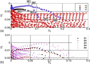
A 共270⫻55兲 grid discretizing a domain of lengths Lx = 450, Ly= 25 for D1, D2, D3 and Lx= 450, Ly= 30 for D4, D5, and a 2000 modes Krylov subspace are assumed throughout the rest of the paper. The lengths of the compu-tational domains have been proven to be large enough to not influence the stability results. The previously mentioned dis-cretization yields to large, quite converged spectra for all the base flows, which are shown in Fig.3. One can observe that all the temporal modes are damped temporally which indi-cates that the considered separated flows are asymptotically globally stable. In particular, the different base flows 共D1– D5兲 span many configurations, from widely stable to margin-ally stable flows.

Three families of temporal modes, referenced as F1, F2, and F3 and described briefly hereafter, could be recovered in the spectra. The least damped modes denoted by F1 and represented by diamonds in the top frame of Fig.3are remi-niscent of classical Kelvin–Helmholtz共KH兲 waves along the shear layer, and relax to Tollmien–Schlichting waves on the attached boundary layer. The eigenvectors of the typical modes labeled M1 and M2 in Fig.3are shown in Figs.4共a兲 and4共b兲. A second category of modes referenced as F2 and represented by squares in the top frame of Fig.3are charac-terized by a spatial distribution reaching the outflow bound-ary, as depicted in Figs.4共c兲and4共d兲, which show the modes labeled M3 and M4 in Fig.3. Finally, a wide range of highly damped modes are classified into F3. This last set of modes

are reminiscent of the so-called continuous branch obtained by a local analysis. Indeed, a part of the energy of the cor-responding modes is concentrated at high values of y. Fur-thermore, one may observe that KH waves are present on the shear layer as shown in Figs. 4共e兲 and 4共f兲, depicting the modes M5 and M6, respectively. Looking at Figs.4共a兲–4共f兲, one can notice the strong similarity in terms of spatial struc-ture of the eigenmodes characterized by close frequencies for F1, F2, and F3. Such a property reveals the strong nonor-thogonality of the eigenvectors for the considered flow, which seems to be a typical feature of open flows and, in particular, of separated flows.24,26 In Sec. III B we would investigate how the non-normality of the temporal modes could affect the linear asymptotic instability of the consid-ered flow subject to a harmonic forcing.

B. Sensitivity associated with the non-normality: Pseudoresonance

In this section, we will investigate briefly the non-normality features of the linearized Navier–Stokes operator and their consequences on the asymptotic behavior of the separated flows. Indeed, even if all the modes are damped temporally, the flow, being strongly separated, is subject to convective instabilities. Thus, the existence of convective waves as a response to a harmonic forcingF=f共x,y兲e−i⍀ft_is

investigated in a global framework. Such a phenomenon may be related to a pseudoresonance of the temporal modes due to the non-normality of the linearized Navier–Stokes opera-tor for the considered flow.37 In order to investigate such a possibility, let us introduce the pseudospectrum of the operator,

␭_␧=兵␴苸 C,储P共␴兲储 ⱖ ␧−1其,

共8兲

with P共␴兲 = 共i␴B − A兲−1_,

which characterizes the asymptotic behavior of the evolution Eq. 共4兲.37 In the present computations an approximation of the pseudospectrum with the Hessenberg matrix from the Arnoldi computation is used.21,38

M5 M1 M2 M3 M4 M6 Ωr Ωi 0 0.1 0.2 0.3 -0.06 -0.04 -0.02 0 F3 F2 F1 (a) (b) Ωr Ωi 0 0.05 0.1 0.15 0.2 -0.02 -0.01 0 0.01 D1 D2 D3 D4 D5

FIG. 3.共Color online兲 共a兲 Spectrum of the separated flow D3 at Re_␦= 200 and Lx= 450. 共b兲 A zoom on the least damped area of the spectrum for

D1–D5.

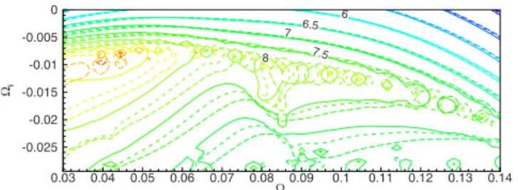
The base flow D1 is considered. As shown in Fig. 5, large sensitivity areas appear around each temporal mode. A pseudoresonance, resulting from the high nonorthogonality, may thus occur even far away from the considered modes. In particular, the value of the contour −log10共␧兲 crossing the real pulsation axis represents the sensitivity of the flow to external disturbances at a given real pulsation ⍀f; a high value of such parameter共⬇10−6_{for the case here considered兲} means that the flow is able to get a large response to an external real forcing at a selected frequency⍀f. Furthermore, it is worth to notice that such a value does not depend on the domain size, as shown by the␧ levels in Fig.5, so that one can argue that it is an intrinsic property of the separated flow. Following the arguments above, we will now investigate in detail the shape of the perturbation inducing an optimal re-sponse to a harmonic forcing and the associated sensitivity mechanism for the flow here considered.

C. Global space-time response to a localized harmonic forcing

1. Theoretical tools based on temporal mode expansion

The global asymptotic response of a perturbation to a harmonic forcing兵F共x,t兲=f共x兲e−i⍀f,⍀f苸R其 can be

formu-lated as a summation of temporal modes as follows:22,37

q共x,t兲 =

兺

k

Kkqˆk共x兲e−i⍀kt, 共9兲

where each couple 共qˆk,⍀k兲 is solution of Eq. 共7兲 and Kk characterize the initial components of the perturbation into the basis composed of temporal modes. The forcing term is expanded in a similar way,

f共x兲 =

兺

k

fkqˆk共x兲. 共10兲

Under the assumption that all the temporal modes are damped temporally, in the asymptotic regime the flow’s re-sponse toF reduces to q共x,t兲 =

兺

We introduce now the quantity R共⍀f兲 which characterizes the maximum response of the separated flow to a forcing,

R共⍀f兲 = max F

储q储E

储F储E, 共12兲

where the energy based norm储 储Eis derived from the scalar product 具q,q典E=兰₀Lx兰

0

Ly共uⴱ_{u +v}ⴱ_v兲dxdy with •ⴱ _{denoting the}

complex conjugate. In order to evaluate Eq.共12兲 we intro-duce the scalar product matrix M whose coefficients are de-fined by (a) (b) (c) (d) (e) (f)

FIG. 4.共Color online兲 Real part of the streamwise component uˆ of the modes labeled in Fig.3as M1–M6. The dividing streamline is illustrated in black. D3 is considered.共a兲 Mode M1. 共b兲 Mode M2. 共c兲 Mode M3. 共d兲 Mode M4. 共e兲 Mode M5. 共f兲 Mode M6.

8 7.5 7 6.5 6 Ωr Ωi 0.03 0.04 0.05 0.06 0.07 0.08 0.09 0.1 0.11 0.12 0.13 0.14 -0.025 -0.02 -0.015 -0.01 -0.005 0

FIG. 5.共Color online兲 Pseudospectrum of the separated flow. The isolevels −log₁₀共␧兲 are shown. Three domain sizes of D1 are studied: L1=450 共—兲,

L2 = 425共- - -兲, and L3=400 共– – –兲 discretized by Nx= 270, 265, and 260

Mi,j=

冕

冕

It is thus more convenient to compute Eq.共12兲as R共⍀f兲 = 储FDfF−1_储

2, 共14兲

with Df_共l,p兲=␦l,p关i/共⍀f−⍀l兲兴 and M=Ft_{F the Cholesky} de-composition of M.

Finally, Eq.共14兲can be computed for each⍀fby deter-mining the largest singular value sv1,

R共⍀f兲 = sv1共FDfF−1兲. 共15兲

The expression of the most responsive disturbance is repre-sented in the temporal mode expansion by the vector Kres which is equal to the right singular vector of FDfF−1 associ-ated with the largest singular value sv1. The components of the forcing term Kf=t共f1, f2, . . . . , fN兲 leading to such a re-sponse can thus be recovered by a simple matrix product

Kf= F−1Kres.

2. Validation of the reduced model

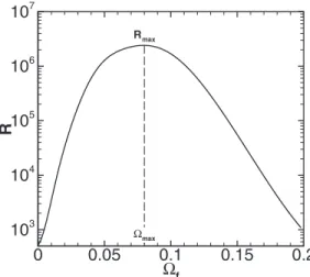
The influence of the number of modes N taken into ac-count in the optimization process is investigated. For that purpose, the base flow D1 is considered. Similar results are provided for the different base flows. The resolvent norm R is plotted in Fig.6 for N = 1300. As it is suggested by the pseudospectrum analysis, one observes a strong amplifica-tion of the value of R which reaches a maximum value for ⍀f= 0.08. In order to validate the behavior predicted by a limited number of modes, two quantities are introduced, de-noted by R_max共N兲 and ⍀_max共N兲,

R_max共N兲 = max_⍀

f关R共⍀f,N兲兴,

共16兲

⍀max共N兲 = 兵⍀f/R共⍀f,N兲 = Rmax共N兲其,

which are sketched in Fig.6. The values of such quantities in function of the number of modes used in the computation of R共⍀f兲 are depicted in Figs. 7共a兲 and 7共b兲. One observes a good convergence of the most amplified frequency which reaches an almost constant value for N = 800. The value of

R_maxexhibits a fast increase for moderate values of N and a slow increase after N = 800. One may expect convergence

when N→⬁.

Therefore, N = 1300 modes are here considered sufficient to capture the optimal response and its associated frequency. The spatial distribution of the optimal forcing and its respec-tive response, both represented by the variable Ux共x兲 =兰₀Ly_u共x,y兲2_{dy, are shown in Figs.8共a兲and8共b兲共the} quanti-ties are normalized by maxx关Ux共x兲兴兲. It appears that a number of modes greater than N = 800 lead to a quite converged spa-tial distribution of the optimal response and forcing, whose u Ωmax R_max Ωf R 0 0.05 0.1 0.15 0.2 103 104 105 106 107

FIG. 6. The resolvent norm R共⍀f兲 is depicted for D1. N=1300 modes are

considered. N Ωma x 200 400 600 800 1000 1200 0.05 0.06 0.07 0.08 N Rma x 200 400 600 800 1000 1200 1E+06 2E+06 3E+06 (a) (b)

FIG. 7. Influence of the dimension of the temporal mode expansion for D1 and Lx= 450.共a兲 Evolution of ⍀maxwith the number of modes.共b兲 Evolution of Rmaxwith the number of modes.

X Ux 0 50 100 150 200 250 300 350 400 0 0.5 1 _N=100 N=300 N=800 N=1300 xr xs X Ux 0 50 100 150 200 250 300 350 400 0 0.5 1 N=100 N=300 N=800 N=1300 (a) (b)

FIG. 8.共Color online兲 Influence of the number of modes N on the spatial distribution of the optimal forcing and response for D1 and Lx= 450. The

vertical lines correspond to the separation point and the reattachment point denoted by Xsand Xrrespectively.共a兲 Streamwise distribution of the optimal

forcing represented by the variable Ux共x兲. 共b兲 Streamwise distribution of the

optimal response represented by the variable Ux共x兲.

components are shown in Figs.9共a兲and9共b兲. One can ob-serve that for N = 1300, the optimal forcing is localized close to the separation point of the bubble leading to a response which is amplified along the shear layer reaching a maxi-mum after the reattachment point. Consequently, it could be argued that the optimal frequency and the corresponding re-sponse are well described by a limited number of modes despite the slow convergence of Rmax. In particular, such a slow convergence may be ascribed to the difficulty to re-cover the tilting of the initial perturbation upstream of the bubble by means of a reduced model based on a global mode expansion. Indeed, the action of the shear on structures tilted at t = 0 in the direction opposed to the mean flow may lead, through an Orr mechanism, to an increase in the energy gain, as observed by Blackburn et al.27 and Marquet et al.28 by means of a direct-adjoint optimal growth strategy. On the other hand, such a mechanism is not perfectly observed in the works of Åkervik et al.24 and Ehrenstein and Gallaire,26 where a global mode expansion strategy is used. Further-more, in the work of Åkervik et al.22on a flat plate boundary layer, it is demonstrated that the Orr mechanism does not affect the value of the optimal response frequency but only the value of the maximum energy gain.

Finally, a validation of the previously discussed results is carried out by means of a perturbative linearized version of the DNS code described in the first part. The equations are written as follows: ⳵␼ ⳵t + U .ⵜ␼ + u . ⵜW = 1 Reⵜ 2_{␼ + F,} 共17兲 ⵜ2_␺=␼,

whereF represents the forcing term, and ␼ and␺the vor-ticity and the stream function perturbation, respectively. The nullity of the velocity fluctuations is imposed all over the boundaries of the computational domain except at the out-flow where the second derivatives of␼ and␺along x are set to zero. A fringe region is implemented in order to damp the perturbation at the outlet.

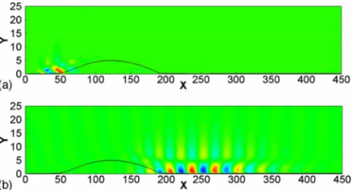
We initialize at zero the perturbation fields and force with two circular frequencies ⍀f= 0.08 and ⍀f= 0.13. The associated forcing field is deduced from the optimization

process. The grid and domain lengths discussed in Sec. II C are used. After the transient, we compare the instantaneous perturbation with the one resulting from the temporal mode expansion with N = 1300. Figures10共a兲and10共b兲 show that the linearized simulation results are in a very good agree-ment with the ones of the linear stability theory based on summation共9兲. Such a computation is a good validation of the temporal mode expansion which has demonstrated to be an appropriate reduced model for the description of the op-timal response to external forcing in the asymptotic regime. Being confident about the results derived from the present summation, we further explore the physical destabilizing mechanism associated with the optimal response.

3. Physical mechanism associated with the optimal response

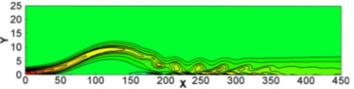
In Fig.11we plot the vector perturbation fields共u,v兲 for ⍀max in the asymptotic regime for the base flow D3. One may observe that the action of the perturbation on the base flow originates a series of counter-rotating vortices along the shear layer and the decelerated zone. A visualization of the instantaneous vorticity field, where ␧ is fixed arbitrarily to 10% of the maximum value of U¯ , represents the resulting response in Fig.12. The destabilizing mechanism associated with the most responsive disturbance described above leads to the formation of rolling vortices amplified along the shear layer which are advected in the attached boundary layer and die away. Such process seems to be a specific feature

under-FIG. 9.共Color online兲 Representation of the streamwise component result-ing from the optimization process. D1 is considered.共a兲 Streamwise com-ponent u of the optimal forcing.共b兲 Streamwise component u of the optimal response.

FIG. 10. Plot of the value of u共x,8兲 obtained by linearized DNS and tem-poral mode expansion with N = 1300 for the base flow D1.共a兲 ⍀f= 0.08.共b兲

⍀f= 0.13.

FIG. 11. 共Color online兲 Illustration of the perturbation vectors 共u,v兲 ob-tained for D3 and the forcing frequency⍀maxin the asymptotic regime. The dividing streamline is represented by the dashed line.

lying the optimal behavior of separated flows. We may for instance refer to the counter-rotating structures observed by Blackburn et al.27 in a flow over a backward facing step resulting from the optimal amplification of a localized wave packet.

In order to determine the effects of the size of the recir-culation area on the values of R共⍀f兲, computations are per-formed for the different base flows discussed in Sec. II C. The response curves are shown in Fig.13.

One can observe the strong increase of the optimal re-sponse value R_max with the size of the recirculation zone which reaches a very high maximum energy gain of order ⬇109 _{for D5. In particular, the most responsive frequency} range is found to reduce when the Reynolds number and/or the pressure gradient at the upper boundary increase, leading to a more defined peak around⍀_max.

Furthermore, Figs. 14–16 show that the spatial support associated with the most responsive disturbance is spreading along the separated zone with the increase in the recircula-tion area. In particular, this last one is centered around the reattachment point for D4. This correlation suggests that an inviscid-type KH mechanism, similar to the one observed in separated flows by Lin and Pauley,39 for instance, is the cause of the increase in the optimal response energy. As de-scribed by the latter, this last one results in the roll-up of the shear layer.

D. Relation between the global optimal response and the onset of unsteadiness

Our analysis has assessed that flat plate separated flows may exhibit a large response to a harmonic forcing for a range of frequencies at moderate Reynolds number. The bubble may act as a selective amplifier of frequencies due to

the strong convectively unstable character of the flow. Fur-thermore, a typical feature of such configuration is the onset of self-sustained oscillations characterized by the triggering of shedded vortices 共see Refs. 16, 30, and 31 in DNS and Ref.40in experiments兲. Moreover, such flows are subject to a certain level of noise in experiments as well as in numeri-cal simulations due to the discretization errors. Therefore, we propose to investigate the connection between the emergence of coherent structures in the considered configuration subject to noise and the amplifier dynamics related to the optimal response to forcing, which leads to the generation of counter-rotating structures, as previously discussed. For that purpose, the full 2D Navier–Stokes equations by superposing a ran-dom noise with small amplitude共10−6_{兲 to the base flow inlet} vorticity are computed. Simulations are carried out for the base flow D5. Figure 17shows a time series and a Fourier analysis of the vorticity component at the wall extracted at two different locations, the reattachment points x = 253 and x = 282; after that the simulation has reached a statistically stationary state. Although a white noise perturbation is im-posed at the inflow, the Fourier spectra shown in Figs.17共b兲 and17共c兲provide a narrow banded response whose peak is localized around ⍀=0.085. This behavior is in agreement with the optimal response analysis realized in Sec. III C 1. In particular, the peak and the range of excited pulsations are close to the predictions of the theoretical analysis based on a temporal modes summation. Similar results are observed with D1–D4.

Thus, we can assume that the amplification mechanism provided by the optimal response analysis is able to describe a possible scenario for the onset of unsteadiness in the con-sidered separated flow. Under a sufficiently large pressure gradient and/or Reynolds number, even a 2D globally stable separated flow is able to select by means of sensitivity an optimal range of frequencies out of the existing numerical noise, generating optimal-like counter-rotating structures which can trigger a self-excited vortex shedding.

This selective noise amplifier mechanism can be com-pared to the unsteadiness taking the form of KH-like shedded

D4 D1 D2 D3 D5 Ωf R 0 0.05 0.1 0.15 0.2 103 104 105 106 107 108 109

FIG. 13. Evolution of R共⍀f兲 for the different separated flows discussed in

Sec. II C. Rmaxare sketched in black points.

FIG. 14.共Color online兲 Streamwise distribution of the optimal response for the base flow D1.

FIG. 15.共Color online兲 Streamwise distribution of the optimal response for the base flow D3.

FIG. 12. 共Color online兲 Instantaneous vorticity for D3 and ⍀max in the asymptotic regime.

vortices observed in the asymptotic regime in numerical simulations of similar configurations by Wasistho et al.,16 Pauley et al.30 and Ripley and Pauley.31

Indeed, such authors observed that under a sufficiently large pressure gradient, a strongly unsteady behavior taking the form of self-excited vortex shedding occurs even at low Reynolds number共Re_␦= 330 for the first one and from 400 to 800 for the last one兲. A natural generation of convective waves from the existing numerical noise is thus suggested by Ref.16as an explanation.

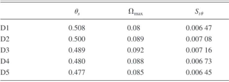
Focusing on the relation between optimal response and the vortex shedding observed in previous investigations, we compute a typical parameter characterizing the unsteadiness behavior such as the shedding frequency nondimensionalized by the boundary layer momentum thickness␪sand the local free stream velocity Ueat the separation point with no ap-plied gradient pressure, through Strouhal number,

St␪= f ␪s Ue

, 共18兲

where f denotes the shedding frequency. According to Pauley et al.,30Ripley and Pauley31and Pauley41for flat plate sepa-rated flows or Lin and Pauley39in an airfoil configuration, a typical Strouhal number associated with unsteadiness varies in the range from 0.0055 to 0.008. It is worth to notice that such a value is not fixed constant due to the dependence of

the shedding frequency to the pressure distribution along the flat plate.31Therefore, the shedding frequency is slightly ge-ometry dependent.

The Strouhal numbers associated with the frequency leading to an optimal response are computed and summa-rized in TableII. Such values are found to be consistent with the ones obtained by the authors previously mentioned.

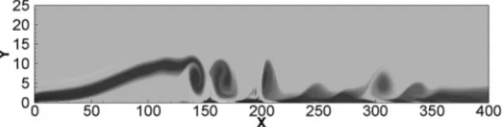
In order to verify that the optimal response is able to trigger unsteadiness in the nonlinear regime, a larger white noise amplitude is superposed at inflow points in a DNS. The base flow D3 is investigated, and the amplitude is fixed to 10−5_{. After the transient, the nonlinear saturation occurs.} Fig-ure 18 shows an instantaneous vorticity field showing the vortex shedding behavior resulting from the selective noise amplifier mechanism at t = 2000. It is worth to notice the strong similarity between the resulting 2D structures and the computations of previous investigations by Refs.16,30, and

31.

Such results support the hypothesis that flat plate sepa-rated flows could act as a selective noise amplifier, whose selected frequencies could be recovered by an optimal re-sponse analysis, and whose amplificating rere-sponse leads to the onset of a self-excited vortex shedding phenomenon.

Nevertheless, as it is detailed in Sec. I of the present manuscript and recently discussed by Marquet et al.,28 a

TABLE II. Values of␪s,⍀max, and St␪at Xsfor the five separated flows.

␪s ⍀max St␪ D1 0.508 0.08 0.006 47 D2 0.500 0.089 0.007 08 D3 0.489 0.092 0.007 16 D4 0.480 0.088 0.006 73 D5 0.477 0.085 0.006 45

FIG. 16.共Color online兲 Streamwise distribution of the optimal response for the base flow D4.

t W a ll v o rt ic it y 0 2000 4000 6000 8000 -1 -0.5 0 0.5 1 (a) Ω nor m a li z e d s tr e ngth 0 0.05 0.1 0.15 0.2 0 0.2 0.4 0.6 0.8 1 (b) _Ω nor m a li z e d s tr e ngt h 0 0.05 0.1 0.15 0.2 0 0.2 0.4 0.6 0.8 1 (c)

FIG. 17. Vorticity histories at the wall taken at two different positions where the inflow condition is continually per-turbed with a low-amplitude random noise. The normalized optimal re-sponse to a localized harmonic forcing is depicted in black line. D5 is consid-ered.共a兲 Time series of the wall vor-ticity at the reattachment point x = 253 extracted from the DNS.共b兲 Normal-ized pulsation distribution from Fou-rier analysis of the wall vorticity his-tory at the reattachment point x = 253. 共c兲 Normalized pulsation distribution from Fourier analysis of the wall vor-ticity history after the reattachment point x = 282.

resonator dynamics associated with a three-dimensional glo-bal stationary unstable mode may occur in separated flows as it is observed in a similar configuration by Theofilis et al.13It may be supposed that such three-dimensional mechanism could appear in the present configuration. Therefore, one can argue that such resonator dynamics could dominate the asymptotic space-time dynamics of the considered flow and invalidate the present analysis. However, Gallaire et al.,15 Marquet et al.,28and Blackburn et al.27established that such three-dimensional global mode is amplified with a weak tem-poral growth rate. Furthermore, the analysis of the influence of random noise perturbation superposed at the inflow in a similar configuration by Pauley42 illustrates that the vortex shedding frequency observed in the 2D computation is not altered by the influence of a three dimensionality of the flow. Thus, it may be suggested that the selective noise amplifier associated with the optimal response yields a convincing sce-nario for the onset of unsteadiness in flat plate separated flows excited by a permanent external noise.

Consequently, the global analysis based on temporal mode expansion seems to be efficient in modeling the asymptotic behavior of open flows which are found to be strongly sensitive to external forcing, opening new

possibili-ties of control strategy aiming at minimize the quantity R共⍀f兲 by reducing the non-normality of the operator.43

IV. CONCLUSION

Recently, global linear stability analyses have yielded a rich picture of the instability features of separated flows. In particular, the concept of non-normality in a global frame-work has explained some large transient phenomena occur-ring even at low Reynolds number. Therefore, as argued by Marquet et al.28and Blackburn et al.,27the amplifier dynam-ics predicted by an optimal growth analysis yields a possible scenario explaining the onset of unsteadiness in flows over a backward facing step under the influence of a localized dis-turbance. Nevertheless, it seems interesting to adopt a differ-ent point of view connecting the triggering of unsteadiness in the asymptotic regime and the selective noise amplifier be-havior of a separated flow. For that purpose, in this work we have studied the global linear response to a localized har-monic forcing leading to a maximum kinetic energy gain in the asymptotic regime, as well as the associated amplifica-tion mechanism and its connecamplifica-tion with the onset of un-steadiness in flat plate separated flows.

The proposed global linear stability approach is found to be able to identify the instability mechanism related to the linear response to a harmonic forcing introduced into a lami-nar flat plate separated flow. In particular, the temporal mode expansion of the perturbation is able to describe the linear space-time dynamics of a 2D perturbation, outlining a desta-bilizing mechanism involving the shear layer. Indeed, the most responsive disturbance takes the form of KH-like vor-tices, which roll up and amplify themselves along the shear layer, until being advected and die away in the attached

TABLE III. Vtop共x兲.

x 0 10 20 30 40 50 60 70 80 90 D1 0.0227 0.0249 0.0308 0.0418 0.0614 0.0900 0.1155 0.1241 0.0097 0.0068 D2 0.0253 0.0277 0.0343 0.0467 0.0688 0.0983 0.1254 0.1352 0.1083 0.0789 D3 0.0295 0.0323 0.0401 0.0544 0.0780 0.1110 0.1406 0.1523 0.1266 0.0974 100 110 120 130 140 150 160 170 180 190 D1 0.0445 0.0233 0.0029 ⫺0.0164 ⫺0.0329 ⫺0.0448 ⫺0.0532 ⫺0.0529 ⫺0.0411 ⫺0.0263 D2 0.0547 0.0315 0.0084 ⫺0.0142 ⫺0.0357 ⫺0.0546 ⫺0.0685 ⫺0.0734 ⫺0.0670 ⫺0.0523 D3 0.0722 0.0470 0.0206 ⫺0.0066 ⫺0.0335 ⫺0.0597 ⫺0.0862 ⫺0.1041 ⫺0.1014 ⫺0.0813 200 210 220 230 240 250 260 270 280 290 D1 ⫺0.0149 ⫺0.0077 ⫺0.0043 ⫺0.0030 ⫺0.0013 0.0014 0.0036 0.0042 0.0038 0.0032 D2 ⫺0.0355 ⫺0.0212 ⫺0.0108 ⫺0.0039 0.0003 0.0028 0.0041 0.0048 0.0050 0.0050 D3 ⫺0.0557 ⫺0.0337 ⫺0.0187 ⫺0.0096 ⫺0.0034 ⫺0.0012 0.0041 0.0053 0.0054 0.0051 300 310 320 330 340 350 360 370 380 390 D1 0.0028 0.0027 0.0027 0.0027 0.0026 0.0025 0.0024 0.0024 0.0023 0.0023 D2 0.0049 0.0047 0.0045 0.0042 0.0040 0.0038 0.0037 0.0035 0.0034 0.0033 D3 0.0048 0.0047 0.0046 0.0045 0.0043 0.0041 0.0039 0.0037 0.0036 0.0035 FIG. 18. Instantaneous vorticity field from DNS subject to a random white

noise at the inflow. The amplitude is fixed to 10−5_.

boundary layer. The pseudoresonance of the temporal modes due to the non-normality of the temporal evolution operator of the linearized Navier–Stokes equations explains this be-havior. Moreover, an analysis of the evolution of the re-sponse, when the Reynolds number and/or the gradient pres-sure are increased, clarifies the strong influence of the shear layer on the maximum response.

Such elements suggest that flat plate separated flows may act as a strong selective noise amplifier. In order to find out if a connection exist between the global optimal response of the flow and the unsteadiness observed in experiments and DNS, a DNS is carried out in which the base flow is con-tinuously perturbed at inlet points with a random noise. The DNS results show that the selected frequencies recovered by Fourier transform in the asymptotic regime are in agreement with the amplified frequencies derived from the optimal re-sponse analysis. The most amplified frequency is then com-pared to the shedding frequencies measured by Pauley et al.,30Ripley and Pauley,31Lin and Pauley,39and Wasistho et al.16The Strouhal number recovered by the authors previ-ously mentioned is found consistent with the most amplified frequency of the global optimal response.

Finally, the present analysis should be completed by tak-ing into account the influence of three-dimensional perturba-tions. The emergence of a resonator dynamics associated with a stationary unstable global mode is expected.13 There-fore, the asymptotic dynamics of such flow is still a challeng-ing problem where the amplifier and the resonator dynamics may compete.

ACKNOWLEDGMENTS

The authors would like to thank Ulrich Rist for welcom-ing Frédéric Alizard into the IAG and for his financial sup-port. We would like to acknowledge the anonymous referees for enlightening discussions, their comments, and advice. Computing time was provided by “Institut du Développe-ment et des Ressources en Informatique Scientifique 共IDRIS兲-CNRS.”

APPENDIX A: SUCTION VELOCITY PROFILES: Vtop„x…

Table III defines the values taken by Vtop along some streamwise position x.

APPENDIX B: COMPUTATIONAL BOX DEPENDENCY

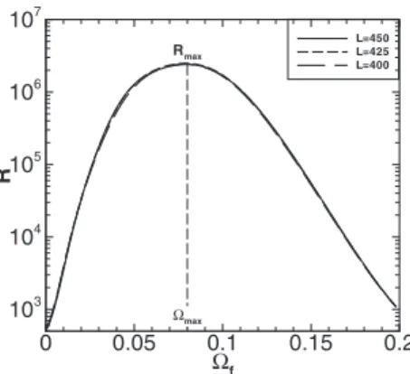
This appendix is devoted to the analysis of the depen-dency of the stability results on the computational box. The case D1 is considered. From Figs.19and20, one observes that despite the spectrum is influenced by the domain size, the resulting resolvent norm is unchanged. The global values are thus independent of the computational box.

1_{B. M. Jones, “Stalling,” J. R. Aeronaut. Soc. 38, 753共1934兲.}

2_{M. Gaster, “The structure and behaviour of laminar separation bubbles,”} Ministry of Technology, Aeronautical Research Council Technical Report No. 3595, 1969.

3_{W. R. Briley, “A numerical study of laminar separation bubbles using the} Navier–Stokes equations,”J. Fluid Mech. 47, 713共1971兲.

4_{V. Sychev, A. I. Ruban, V. Sychev, and G. L. Korolev, Asymptotic Theory}

of Separated Flows共Springer, New York, 2005兲.

5_{U. Rist and U. Maucher, “Direct numerical simulation of 2-d and 3-d} instability waves in a laminar separation bubble,” AGARD Conf. Proc.

551, 361共1994兲.

6_{U. Rist and U. Maucher, “Investigations of time-growing instabilities in} laminar separation bubbles,”Eur. J. Mech. B/Fluids 21, 495共2002兲.

7_{A. V. Dovgal, V. V. Kozlov, and A. Michalke, “Laminar boundary layer} separation: Instability and associated phenomena,”Prog. Aerosp. Sci. 30,

61共1994兲.

8_{B. F. Armaly, F. Durst, J. C. F. Pereira, and B. Schönung, “Experimental} and theoretical investigation of backward-facing step flow,”J. Fluid Mech.

127, 473共1983兲.

9_{L. Kaiktsis, G. Karniadakis, and A. Orszag, “Unsteadiness and convective} instabilities in two-dimensional flow over a backward-facing step,” J.

Fluid Mech. 321, 157共1996兲.

10_{P. Huerre and P. A. Monkewitz, “Absolute and convective instabilities in} free shear layers,”J. Fluid Mech. 159, 151共1985兲.

11_{M. Marquillie and U. Ehrenstein, “On the onset of nonlinear oscillations in} a separating boundary-layer flow,”J. Fluid Mech. 490, 169共2003兲.

12_{B. Pier, “On the frequency selection of finite-amplitude vortex shedding in} the cylinder wake,”J. Fluid Mech. 458, 407共2002兲.

13_{V. Theofilis, S. Hein, and U. Dallmann, “On the origins of unsteadiness} and three dimensionality in a laminar separation bubble,”Philos. Trans. R.

Soc. London, Ser. A 358, 3229共2000兲.

14_{D. Barkley, M. Gomes, and D. H. Genderson, “Three dimensional} insta-bility in flow over a backward-facing step,”J. Fluid Mech. 473, 167

共2002兲.

15_{F. Gallaire, M. Marquillie, and U. Ehrenstein, “Three-dimensional} trans-verse instabilities in detached boundary layers,”J. Fluid Mech. 571, 221

共2007兲.

16_{B. Wasistho, B. J. Geurts, and J. G. M. Kuerten, “Numerical simulation of} separated boundary-layer flow,”J. Eng. Math. 32, 177共1997兲.

17_{V. Theofilis, “Advances in global linear instability of nonparallel and} three-dimensional flows,”Prog. Aerosp. Sci. 39, 249共2003兲.

18_{C. Cossu and J.-M. Chomaz, “Global measures of local convective}

insta-Ωr Ωi 0 0.05 0.1 0.15 0.2 -0.04 -0.02 0 0.02 L=450 L=425 L=400

FIG. 19.共Color online兲 Influence of the computational box on the spectrum. D1 is considered. Ωmax Rmax Ωf R 0 0.05 0.1 0.15 0.2 103 104 105 106 107 L=450 L=425 L=400

FIG. 20. The resolvent norm R共⍀f兲 is depicted for D1 where 1300 modes

are considered. Three computational boxes are studied referenced by Lx

= 450, Lx= 425, and Lx= 400 associated with Nx= 270, Nx= 265, and Nx

bilities,”Phys. Rev. Lett. 78, 4387共1997兲.

19_{J.-M. Chomaz, “Global instabilities in spatially developing flows:} Non-normality and non linearity,”Annu. Rev. Fluid Mech. 37, 357共2005兲.

20_{U. Ehrenstein and F. Gallaire, “On two dimensional temporal modes in} spatially evolving open flows: The flat-plate boundary layer,”J. Fluid

Mech. 536, 209共2005兲.

21_{F. Alizard and J.-C. Robinet, “Spatially convective global modes in a} boundary layer,”Phys. Fluids 19, 114105共2007兲.

22_{E. Åkervik, U. Ehrenstein, F. Gallaire, and D. S. Henningson, “Global} two-dimensional stability measures of the flat plate boundary-layer flow,”

Eur. J. Mech. B/Fluids 27, 501共2008兲.

23_{P. J. Schmid and D. Henningson, “On the stability of a falling liquid} curtain,”J. Fluid Mech. 463, 163共2002兲.

24_{E. Åkervik, J. Hoepffner, U. Ehrenstein, and D. S. Henningson, “Optimal} growth, model reduction and control in a separated boundary-layer flow using global eigenmodes,”J. Fluid Mech. 579, 305共2007兲.

25_{D. S. Henningson and E. Åkervik, “The use of global modes to understand} transition and perform flow control,”Phys. Fluids 20, 031302共2008兲.

26_{U. Ehrenstein and F. Gallaire, “Global low-frequency oscillations in a} separating boundary-layer flow,”J. Fluid Mech. 614, 315共2008兲.

27_{H. M. Blackburn, D. Barkley, and S. J. Sherwin, “Convective instability} and transient growth in flow over a backward-facing step,”J. Fluid Mech.

603, 271共2008兲.

28_{O. Marquet, D. Sipp, J.-M. Chomaz, and L. Jacquin, “Amplifier and} reso-nator dynamics of a low-Reynolds-number recirculation bubble in a global framework,”J. Fluid Mech. 605, 429共2008兲.

29_{P. J. Schmid, “Nonmodal stability theory,”Annu. Rev. Fluid Mech. 39,} 129共2007兲.

30_{L. L. Pauley, P. Moin, and W. Reynolds, “The structure of two} dimen-sional separation,”J. Fluid Mech. 220, 397共1990兲.

31_{M. D. Ripley and L. L. Pauley, “The unsteady structure of} two-dimensional steady laminar separation,”Phys. Fluids A 5, 3099共1993兲.

32_{O. Daube, “Resolution of the 2D Navier–Stokes equations in} velocity-vorticity form by means of an influence matrix technique,”J. Comput.

Phys. 103, 402共1992兲.

33_{R. Peyret, Spectral Methods for Incompressible Viscous Flow共Springer,} New York, 2002兲.

34_{M. Pernice and F. W. Homer, “Nitsol: A Newton iterative solver for} non-linear systems,”SIAM J. Sci. Comput.共USA兲 19, 302共1998兲.

35_{T. N. Phillips and G. W. Roberts, “The treatment of spurious pressure} modes in spectral incompressible flow calculations,” J. Comput. Phys.

105, 150共1993兲.

36_{R. B. Lehoucq, D.C. Sorensen, and C. Yang,}

ARPACKUsers’ Guide:

Solu-tion of Large Scale Eigenvalue Problems with Implicitly Restarted Arnoldi Methods共SIAM, Philadelphia, 1998兲.

37_{P. J. Schmid and D. S. Henningson, Stability and Transition in Shear}

Flows共Springer, New York, 2001兲.

38_{K.-C. Toh and L. N. Trefethen, “Calculation of pseudospectra by the} Ar-noldi iteration,”SIAM J. Sci. Comput.共USA兲 17, 1共1996兲.

39_{J. C. M. Lin and L. L. Pauley, “Low-Reynolds-number separation on an} airfoil,”AIAA J. 34, 1570共1996兲.

40_{C. P. Häggmark, A. A. Bakchinov, and P. H. Alfredsson, “Experiments on} a two-dimensional laminar separation bubble,” Philos. Trans. R. Soc. Lon-don, Ser. B 358, 3193共2000兲.

41_{L. L. Pauley, “Structure of local pressure-driven three-dimensional} tran-sient boundary-layer separation,”AIAA J. 32, 997共1994兲.

42_{L. L. Pauley, “Response of two-dimensional separation to} three-dimensional disturbances,”ASME J. Fluids Eng. 116, 433共1994兲.

43_{T.-R. Bewley and S. Liu, “Optimal and robust control and estimation of} linear paths to transition,”J. Fluid Mech. 365, 305共1998兲.