Science Arts & Métiers (SAM)
is an open access repository that collects the work of Arts et Métiers Institute of Technology researchers and makes it freely available over the web where possible.
This is an author-deposited version published in: https://sam.ensam.eu Handle ID: .http://hdl.handle.net/10985/9219
To cite this version :
Benjamin LAMOUREUX, Jean-Rémi MASSÉ, Nazih MECHBAL - Improving Aircraft Engines Prognostics and Health Management via Anticipated Model-Based Validation of Health Indicators - Prognostics journal - Vol. 2, n°1, p.18-38 - 2014
Any correspondence concerning this service should be sent to the repository Administrator : archiveouverte@ensam.eu
Improving Aircraft Engines Prognostics and Health Management via
Anticipated Model-Based Validation of Health Indicators
Benjamin Lamoureux benjamin.lamoureux@snecma.fr
Systems Health Monitoring, SAFRAN Snecma
Rond Point René Ravaud, Moissy-Cramayel, Paris area, France
Jean-Rémi Massé jean-remi.masse@snecma.fr
Systems Health Monitoring, SAFRAN Snecma
Rond Point René Ravaud, Moissy-Cramayel, Paris area, France
Nazih Mechbal nazih.mechbal@ensam.eu
PIMM laboratory, Arts & Métiers ParisTech 151 boulevard de l’Hôpital, Paris, France
Abstract
The aircraft engines manufacturing industry is subjected to many dependability constraints from certification authorities and economic background. In particular, the costs induced by unscheduled maintenance and delays and cancellations impose to ensure a minimum level of availability. For this purpose, Prognostics and Health Management (PHM) is used as a means to perform online periodic assessment of the engines’ health status. The whole PHM methodology is based on the processing of some variables reflecting the system’s health status named Health Indicators. The collecting of HI is an on-board embedded task which has to be specified before the entry into service for matters of retrofit costs. However, the current development methodology of PHM systems is considered as a marginal task in the industry and it is observed that most of the time, the set of HI is defined too late and only in a qualitative way. In this paper, the authors propose a novel development methodology for PHM systems centered on an anticipated model-based validation of HI. This validation is based on the use of uncertainties propagation to simulate the distributions of HI including the randomness of parameters. The paper defines also some performance metrics and criteria for the validation of the HI set. Eventually, the methodology is applied to the development of a PHM solution for an aircraft engine actuation loop. It reveals a lack of performance of the original set of HI and allows defining new ones in order to meet the specifications before the entry into service.
Keywords: Prognostics and Health Management, Health Indicators, Validation,
Model-Based, Performance metrics.
1. Introduction
Over the past decades, the importance of dependability within the modern aircraft engines manufacturing industry has grown significantly. The concept of dependability was formalized in the middle 1980s by Jean-Claude Laprie [1]. According the concept he developed with Avizienis, dependability is composed of three elements: attributes, threats and means.
In the field of aircraft engines, attributes are commonly safety, reliability, maintenability and availability, threats are faults and failures and means are removal, prevention, tolerance and forecasting. Dependability constraints generally come from certification authorities and economic background: While certification authorities impose a minimum level of safety and reliability, economy imposes a high level of maintenability and availability. The dependability management of aircraft engines is currently organized as follows:
Removal is used to increase engines’ safety and reliability via corrective maintenance Prevention is used to increase engines’ safety and reliability via preventive maintenance Tolerance is used to increase engines’ safety via fault tolerant control and dispatch
Forecasting is still a research subject because the computational capabilities to perform it were not available before the advent of embedded systems and large scale networks
If we take a look at the operating costs repartition (see Fig. 1), the importance of direct maintenance costs traduces that the current dependability management strategy based on corrective and preventive maintenance entails high direct maintenance costs that are becoming prohibitive and could be reduced. Those costs come mainly from the following ascertainment: The interval between preventive maintenance check-up is not optimized and entails many
additional costs with growing size of fleets.
Tolerance logics result on a multiplication of faults occurrence which are often false alarms resulting on No Fault Found (NFF).
Aircraft engines are becoming more and more electric and as a result the number of potential causes of failure increases. The current troubleshooting process is becoming obsolete because not too much based on reliability analysis and not enough on physical considerations.
In cases of no-dispatch alarms or unpredicted failure, the costs can be very high in cases where the aircraft is blocked in an isolated airport with rudimentary maintenance center.
Corrective maintenance results on Delays and Cancellations (D&C) which entails high indirect costs because of indemnification to passengers.
Eventually, the stock of spare parts, the size of fleets and the maintenance infrastructures must be over dimensioned because of previous consideration.
In order to limit those costs, one is to increase maintenability and availability by use of forecasting, i.e. the ability to anticipate faults and failures and to avoid their unexpected appearance. Fault forecasting made a remarkable entry in the scientific world at the end of the
1990s. At first, it was dedicated to structures through Structural Health Monitoring (SHM) [2] but has spread to other fields with an additional management aspect to make a link between monitoring and maintenance. Prognostics and Health Management (PHM) [3] is the application of health monitoring to systems with a supervision aspect enabling new kind of maintenance strategies such as condition-based maintenance [4] or predictive maintenance. PHM is the most used term but other can be found such as Health and Usage Monitoring Systems (HUMS) or Systems Health Management (SHM).
The upper purpose of PHM is to improve systems availability and maintenability in order to be complementary to removal, prevention and tolerance in dependability management. For this aim, it performs diagnostics and prognostics from a set of variables reflecting the health status of the host system named Health Indicators (HI). The set of health indicators should be capable of: Detecting degradation modes occurring in the host system
Identify threat precursors
Localize the degrading functional unit
Prognose the Remaining Useful Life (RUL) before threat occurrence
These HI are the keystone of PHM: a bad selection will ensure bad performances for the PHM system. Moreover, because of prohibitive controller retrofit costs in aircraft engines industry, the embedded part of PHM including the computation of HI should be validated before the entry into service. Eventually, the selection and validation of HI is a paramount step which needs to be undertaken in the earliest development stages. However, despite its importance, the issue of selecting and validating HI is rarely addressed in the scientific community. Actually, as far as the selection is concerned, there are research papers addressing structural residuals or parity spaces [5], but although the introduced methods perform well on simple simulated systems, they are not applicable to real operating complex systems such as aircraft engines with specific constraints such as imposed location and type of sensors, highly impacting environment, limited embedded computational and storage capacities, high development costs and certifications. Concerning the validation of HI, there is currently no method to validate them independently so they are validated during the latest development stages, simultaneously with the whole PHM system. It means that in the current framework, one has to wait for the host system to have experiment every type of faults and failures several to be able to validate the PHM system and by the same the set of HI. Obviously, given the level of aircraft engines reliability, it can take decades, which is not acceptable.
In the light of the previous observation, the aircraft engines industry could find great interest in a methodology aimed at selecting and validating HI during design phases. This paper proposes such a methodology, based on physics based modeling of the host system and uncertainties propagation to create stochastic data. The selection is based on expert knowledge, experience feedback, equipment specifications and acceptance test procedures descriptions. The validation is based on the computation of four types of Numerical Key Performance Indicators (NKPI) assessing the potential of the HI set for respectively the detection of degradation modes, the identification of incoming threats’ precursors, the localization of degrading functional unit and the prognostics of the Remaining Useful Lifetime (RUL) of the system before the occurrence of next threat.
The remainder of this paper is organized as follows: the first section presents the PHM systems development methodology as it is proposed by authors. The second section is dedicated to the
selection and validation of HI. The third section addresses the issue of modeling and uncertainties propagation and the fourth and final section presents the application of the methodology to the PHM of an aircraft engine control loop with a review of the results.
2. Prognostics and Health Management Systems
2.1. The lexical framework of PHMIn the present PHM framework, we consider two kinds of threats: operating threats that are observable because related to external and ascertainable change of the system and physical threats that are not observable because related to internal and hidden change within the system.
Operating threats:
o Failures: Online observation of a loss of system’s operability.
In high safety requirement fields such as aeronautics, failures can be catastrophic if they appear in flight. Thus, a great part of them are “protected” by the definition of faults that play the role of warnings for imminent failures. However, as it is neither possible to predict every potential failure nor to set up a fault detection logic for those we know, failures without faults can occur. o Faults: Online observation of a difference between the real characteristic of an entity and the
specified characteristic, this difference exceeding the limits of acceptability.
Fault are associated with tolerance logics aimed at allowing the aircraft to finish its mission. Then, the removal of the fault depends on its level of dispatch. There are three types of dispatch:
Long-term dispatch faults: Repair or replacement is expected within hundreds of flights Short-term dispatch faults: Repair or replacement is expected within dozens of flights No dispatch faults (or No-go): Repair or replacement is expected immediately on site. Physical threat:
o Degradation Modes: Modifications of one value of the host system’s parameters. Degradation modes are defined by expertise, experience feedback or physical reasoning.
Marginal degradation modes: lead neither to fault nor failures
Hazardous degradation modes: Low hazard degradation modes lead to long-term or short-term dispatch faults and High hazard degradation modes lead to No dispatch faults or failures
Although only hazardous degradation modes have to be monitored for dependability purposes, it is necessary to consider also marginal degradation modes for identification matters because even if they are not dangerous for the system, they can be detected and lead to erroneous diagnostics. The true added value of PHM for dependability management is the consideration of degradation modes which enables forecasting. A given degradation mode leads to one type of operating threat but this is not reciprocal: an operating threat can be the result of different degradation modes. o Intensity: The intensity of a degradation mode is the ratio of the current value of the
degrading parameter over its mean limit value. It is given in percentage.
o Mean Limit Value: For a hazardous degradation mode, it is the value of the degrading
parameter for which the associated operating threat is reached with a probability of 0.5. For a marginal degradation mode, it is the maximal reasonable value that the parameter can take. For degradation mode 𝑗, the MLV is written 𝑀𝐿𝑉𝑗. The mean limit value can be determined by expertise, experience feedback or simulation.
need vectors to collect relevant data from the system. Collecting vectors:
o Health Indicators: Variable issued from a combination of measures, control values, models or
other sources of knowledge that reflects the health status of a system.
o Syndrom: Vector of the set of Health Indicators’ values at the time of observation.
o Precursor: Reference syndrom traducing the presence of a degradation mode. A precursor is
associated with the level of intensity of the running degradation mode. Typically, we consider 25%, 50%, 75% and 100% precursors.
Note that the 100% precursor traduces a state where an operating threat has 0.5 probability to occur.
Finally, we need processing means to traduce the syndroms into meaningful and interpretable information destined to maintenance operators.
Processing means:
o Diagnostics: Set of operations performed to detect and identify most probable degradation
modes and localize degraded system.
o Detection: Send an alert to the support system when one HI at least crosses a threshold. o Identification: Classify the observed syndrom with respect to a precursors’ database to
identify the type of running degradation mode.
o Localization: Determine the degraded sub-system, functional unit, equipment or component
from the identified running degradation mode.
o Prognostics: Set of operations performed to predict the remaining time before next operating
event of a system based on current diagnostics and history data.
2.2. PHM architecture
In the case of aircraft engines, the PHM system is divided into three stations: the collecting, the processing and the scheduling station. The first one is embedded into the host system and in charge of the online computation and storage of HI. The sending of HI is commonly performed at
the end of each flight. The second station is in the Health Monitoring (HM) system and in charge of the offline computation of status indicators. Status indicators are structures broadcasting information about the system health status from the HM system to the support system. The third station is part of the support system and in charge of updating the maintenance plan with respect to the status indicators received from the processing station. The interaction between these stations is shown in Fig. 2. Each station has its own development issues:
Collecting station: Selection and validation of a performing set of HI.
Processing station: Implementation and verification of algorithmic solutions for diagnostics and prognostics.
Scheduling station: Network implementation and database management. Interfaces between processing results and maintenance operators.
Concerning the functioning of PHM, we will consider the following scheme: the Open System Architecture for Condition-Based Maintenance (OSA-CBM). The correspondence between the three stations introduced above and the OSA-CBM steps is given in Fig. 3. In the remainder of this paper, only issues related to the collecting station are addressed. Actually, the scientific production is quite prolific concerning the two other stations, as evidenced by the numerous review papers on diagnostics and prognostics (see [6], [7]). However, all the related applications are, of what we know, run on systems for which the selection of HI is a simple task because industrial constraints are not taken into account. This paper tries to reduce the gap between academic research and industrial expectancies by providing a method for a model-based selection and validation of health indicators in the design stages. It could become a great asset for companies that are currently developing PHM systems with no quantifiable information about the quality of their HI.
3. Development process of the collecting station
As mentioned above, the role of the collecting station is to compute and store HI online. It means that all the collecting algorithms have to be embedded into the controller. In aircraft engines, collecting algorithms are implemented into a dedicated controller named Engine Monitoring Unit (EMU). Because in flight environmental constraints are stringent, the EMU have neither high computational capabilities nor large storage capacities. Moreover, because collecting algorithms have the lowest level of criticality, they do not have the priority for post entry into service
controller updates named retrofit. Finally, the HI set have to be selected and validated at the latest for the end of design stages. This section introduces a methodology to achieve this purpose. 3.1. Health Indicators Selection
The selection consists in establishing a list of HI that seems to be a priori suitable with respect to the list of degradation modes. For this selection, the following items are needed (see Fig. 4): o The functional and organic architecture of the host system
o Results of risk analysis methods o Equipments specifications documents
o Acceptance Test Procedures (ATP) descriptions Functional and organic architecture
3.1.1.
The functional architecture defines the different functions the host system is expected to be able to perform in a hierarchical form. The principal functions of the host system are declined into secondary functions for subsystems and components. The organic architecture shows the different subsystems, functional units and equipments of the system. In the aircraft engines industry, maintenance constraints have forced the arrival of modular architecture. Modular units are set of equipments that are replaceable online. They are named Line Replaceable Unit (LRU). In a PHM purpose, the most important for diagnostics is to be able to localize the degraded LRU because maintenance operators need this information to proceed to its replacement. The knowledge of functional and organic architectures allows determining the list of these LRU.
Risk analysis 3.1.2.
Risk analysis or risk assessment methods aim at determining quantitative or qualitative value of risk. Risk analysis can be based on inductive or deductive reasoning. The most famous method is an inductive reasoning method named Failure Modes and Effects Analysis (FMEA). The purpose of FMEA is to perform a functional analysis of the system and to identify potential failure modes, their causes and their effects. FMEA can be based on every source of knowledge. In aircraft engines development process, FMEA is undertaken during design stages thanks to expertise and experience feedback. Finally, risk analysis methods allow identifying failures and their associated hazardous degradation modes.
Equipment specifications 3.1.3.
Equipments specifications are defined from the functional and organic architecture. They provide lists of requirements which can be of structural type (e.g. lengths, diameters, stiffness…) or of functional type (e.g. min flow, response time, max gap between two values…). The list of requirements contains generally a list of faults with associated detection and tolerance logics which purpose is to protect the system from reaching a failure. Faults are defined by engineers from the results of the risk analysis. In a PHM purpose, we want to prevent those faults from occurring because they often entail expensive delays and cancellations, a fortiori when they are of no dispatch type. Equipment specifications documents allow identifying faults and their associated hazardous degradation modes.
Acceptance test procedures 3.1.4.
In aircraft engines industry, Acceptance Test Procedures (ATP) are series of test run on equipments or subsystems received from suppliers to check if they comply to specification in order to be able to enter into service. The same tests are also used during maintenance check-ups. Thus, ATP are a good source of ideas for the definition of HI. Beyond the precious information they give, the interest to use ATP is that they are already used and mastered by maintenance operators so that HI based on ATP will have a better welcome due to a better understanding. 3.2. Health Indicators Validation
The validation consists in verifying if the established list of HI is capable of detecting and identifying precursors, localizing degraded LRU and predicting threat occurrence in compliance with performance metrics. For this validation, the following items are needed:
o List of Line Replaceable Units (LRU)
o List of degradation modes and their correspondence with LRU o Physics-based models of the host system and its subsystems o Performance metrics for the validation
o Specifications of required values of the performance metrics List of line replaceable units
3.2.1.
Because the final objective of PHM is maintenance, the localization of degraded LRU is the most important feature of the diagnostics. Therefore, the list of LRU is of paramount importance. It is obtained from the organic architecture knowledge (see Fig. 4).
List of degradation modes 3.2.2.
One of the PHM objectives being to detect and identify hazardous degradation modes, it is necessary to have the list of these degradation modes. The list of hazardous ones come from risk analysis and equipment specifications as explained above. However, it is not sufficient as we need to consider also the marginal degradation modes in order to validate the identification. The list of marginal degradation modes can be established thanks to an analysis of the model’s parameters combined with scientific publications and expert advices.
Physics-based models 3.2.3.
The physics-based model of the system can be built as soon as the organic architecture of the host system is adopted. Then, the values of the parameters are determined via equipment specifications.
Performance metrics 3.2.4.
In order to assess the quality of the HI, some performance metrics are needed. The principal performance metrics are detectability, identificability, localizability and prognosticability defined from Receiver Operating Characteristic (ROC) curves and introduced in the next section.
HI performance requirements 3.2.5.
compared to some performance requirements: 𝑇𝑃𝑆𝑃𝐸𝐶 and 𝐹𝑃𝑆𝑃𝐸𝐶, respectively the specified minimal true positive and maximal false positive ratio, 𝐷𝐻%, 𝐼𝐻%, 𝐿𝑈% and 𝑃𝐻%, the percentage of respectively detectable hazardous degradation modes, identifiable hazardous degradation modes, localizable LRU and prognosticable hazardous degradation modes.
4. Performance Metrics
In order to quantify the potential of the set of HI to meet the specifications, the authors have defined some performance metrics called Numerical Key Performance Indicators (NKPI). The main particularity of these NKPI is that they can be computed as soon the design phases because their calculation only needs distributions of HI characterizing healthy and degraded states. These distributions can be computed via uncertainties propagation on a model. The NKPI are defined from Receiver Operating Characteristics (ROC) curves [8], a well-known graphical tool in signal detection theory [9] which illustrates the performance of a binary classifier. ROC curves are created by plotting the rate of False Positive (FP) versus the rate of True Positive (TP) for varying discrimination thresholds. In practice, ROC curves are drawn from two distributions of a given HI 𝑖; the first one representing the nominal state noted 𝑇𝑖0, and the second one representing a degraded state resulting of degradation mode 𝑗 named 𝑇𝑖,𝑗𝑚 with 𝑚 the degrading parameter’s value. In the remainder of this paper, ℎ is the number of HI and 𝑑 the number of degradation modes, so that (𝑖, 𝑗) ∈ ⟦1; h⟧ × ⟦1; d⟧.
4.1. Detectability matrix
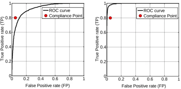
For each couple (HI/degradation mode), the detectability index indicates if the HI is capable of detecting the degradation mode at its mean limit value within false positive and true positive specifications. In practice, we draw the ROC curve between the nominal distribution of the HI and the 100% precursor distribution of the HI and compute the Detectability index as following:
𝐷(𝑇, 𝑇′) = {1 𝑖𝑓 𝑅𝑂𝐶(𝑇, 𝑇′) 𝑖𝑠 𝑎𝑏𝑜𝑣𝑒 𝑡ℎ𝑒 𝑐𝑜𝑚𝑝𝑙𝑖𝑎𝑛𝑐𝑒 𝑝𝑜𝑖𝑛𝑡
0 𝑖𝑓 𝑅𝑂𝐶(𝑇, 𝑇′) 𝑖𝑠 𝑢𝑛𝑑𝑒𝑟 𝑡ℎ𝑒 𝑐𝑜𝑚𝑝𝑙𝑖𝑎𝑛𝑐𝑒 𝑝𝑜𝑖𝑛𝑡 (1)
Where the compliance point is defined as the point of coordinates (𝐹𝑃𝑆𝑃𝐸𝐶, 𝑇𝑃𝑆𝑃𝐸𝐶) (see Fig. 5). Detectability indices are computed for each couple (𝑇𝑖0, 𝑇𝑖,𝑗𝑀𝐿𝑉𝑗) , (𝑖, 𝑗) ∈ ⟦1; h⟧ × ⟦1; d⟧ with the value of the degrading parameter equal to 𝑀𝐿𝑉𝑗 to construct the detectability matrix 𝑫.
𝑫 = | 𝐷(𝑇10, 𝑇1,1𝑀𝐿𝑉1) … 𝐷(𝑇ℎ0, 𝑇ℎ,1𝑀𝐿𝑉 1 ) ⋮ ⋱ ⋮ 𝐷 (𝑇10, 𝑇1,𝑑𝑀𝐿𝑉 𝑑 ) … 𝐷 (𝑇ℎ0, 𝑇ℎ,𝑑𝑀𝐿𝑉 𝑑 ) | ∈ {0,1}𝑑×ℎ (2)
We can now define the notion of detectability for degradation modes: a degradation mode is said “detectable” when its corresponding column of 𝑫 is non-null.
4.2. Identificability Matrix
Before introducing the identificability matrix, we need to define signatures. The signature matrix 𝑺𝒊𝒈 is defined as follows: 𝑺𝒊𝒈 = || 𝑠 (𝑚 (𝑻𝟏,𝟏𝑴𝑳𝑽𝟏) − 𝑚(𝑻𝟏𝟎)) 𝐷(𝑇10, 𝑇1,1𝑀𝐿𝑉1) ⋯ 𝑠 (𝑚 (𝑻𝒉,𝟏𝑴𝑳𝑽 𝟏 ) − 𝑚(𝑻𝒉𝟎)) 𝐷(𝑇ℎ0, 𝑇ℎ,1𝑀𝐿𝑉 1 ) ⋮ ⋱ ⋮ 𝑠 (𝑚 (𝑻𝟏,𝒅𝑴𝑳𝑽 𝒅 ) − 𝑚(𝑻𝟏𝟎)) 𝐷 (𝑇10, 𝑇1,𝑑𝑀𝐿𝑉 𝑑 ) ⋯ 𝑠 (𝑚 (𝑻𝒉,𝒅𝑴𝑳𝑽 𝒅 ) − 𝑚(𝑻𝒉𝟎)) 𝐷 (𝑇ℎ0, 𝑇ℎ,𝑑𝑀𝐿𝑉 𝑑 ) || (3)
Where 𝑚(. ) is the function computing the median of a distribution and 𝑠(. ) is the sign function. For degradation mode 𝑗, the signature 𝑺𝒊𝒈𝑗 is the vectors corresponding to the jth row of 𝑺𝒊𝒈.
Supposing that the set of signatures forms a Euclidian space 𝒯, the identificability index is defined for a couple of degradation modes (𝑗, 𝑘) as the ratio of the angular deviation between signatures over the optimal angular deviation.
𝐼(𝑗, 𝑘) =𝟏𝝅𝑎𝑟𝑐𝑐𝑜𝑠 (‖𝑺𝒊𝒈𝑺𝒊𝒈𝒋‖𝑗𝑻∙𝑺𝒊𝒈𝒌
𝓣‖𝑺𝒊𝒈𝒌‖𝓣)
(4)
Identificability indices are then computed for each couples of degradation modes (𝑗, 𝑘) ∈ ⟦1; d⟧2 to construct the symmetric identificability matrix 𝑰.
Fig. 5: Compliance Point and ROC curve for non-compliant HI (left) and
compliant HI (right) 0 0.2 0.4 0.6 0.8 1 0 0.2 0.4 0.6 0.8 1
False Positive rate (FP)
T ru e P o si tive r a te ( T P ) 0 0.2 0.4 0.6 0.8 1 0 0.2 0.4 0.6 0.8 1
False Positive rate (FP)
T ru e P o si tive r a te ( T P ) ROC curve Compliance Point ROC curve Compliance Point
𝑰 = |𝐼(1, 1) … 𝐼(1, 𝑑)⋮ ⋱ ⋮
𝐼(𝑑, 1) … 𝐼(𝑑, 𝑑)| ∈ [0; 1]
𝑑×𝑑 (5)
We can now define the notion of identificability for degradation modes: a degradation modes is said “identifiable” when its corresponding column of 𝑰 has no coefficient equal to 0 except the one of the diagonal.
4.3. Localizability Matrix
Before introducing the localizability matrix, we need to define the notion of LRU matrix. The LRU matrix associates each degradation mode to the LRU to which it belongs. It allows localizing the degraded LRU from the identified degradation mode. The LRU matrix is defined as follows:
𝑼 = |𝑢(1, 1) … 𝑢(1, 𝑙)⋮ ⋱ ⋮
𝑢(𝑑, 1) … 𝑢(𝑑, 𝑙)| ∈ {0; 1}
𝑑×𝑙 (6)
Where 𝑙 is the number of LRU composing the system and 𝑢(𝑗, 𝑟) is equal either to 1 if degradation mode 𝑗 is affecting LRU 𝑟 or equal to 0 if not.
The localizability matrix 𝑳 is then defined as follows:
𝑳 = 𝑼𝑻𝑰𝑼 ∈ [0; 1]𝑙×𝑙 (7)
We can now define the notion of localizability for LRU: a LRU is said “localizable” when its corresponding column of 𝑳 has no coefficient equal to 0 except the one of the diagonal.
4.4. Prognosticability Vector
Before introducing the prognosticability matrix, we need to define the notions of Minimal Detectable Value (MDV). For a given degradation mode, the MDV is the minimal value of the degrading parameter for which at least one of the HI has a detectability equal to 1. For degradation mode 𝑗, the MDV is written 𝑀𝐷𝑉𝑗. The prognosticability vector 𝑷 is defined for each degradation mode j ∈ ⟦1; d⟧ as follows:
𝑷 = |∆(1) … ∆(𝑑)|𝑻∈ [0; 1]𝑑 (8)
Where and ∆(𝑗) is the relative detection margin equal to:
∆(𝑗) = 𝑀𝐿𝑉 𝑀𝐿𝑉𝑗−𝑀𝐷𝑉𝑗 𝑗 (9)
We can now define the notion of prognosticability for degradation modes: a degradation mode is said “prognosticable” when its corresponding line of 𝑷 is non-null. In other terms, a degradation mode is “prognosticable” if it exists a 𝑛% precursor that is detectable, with 𝑛 < 100%. Because it needs a MLV, prognosticability is computable only for hazardous degradation modes.
4.5. Final Validation
In the end, the set of HI is validated with respect to the following criteria: 𝐷𝐻%, 𝐼𝐻% and 𝑃𝐻% the percentages of respectively detectable, identificable and prognosticable
hazardous degradation modes and 𝐿𝑈% the percentage of localizable LRU.
5. Modeling and Uncertainties Propagation
5.1. System’s modelingLet’s suppose that the physics-based model is represented by a deterministic function 𝒻:
𝒀 = 𝒻(𝑼, 𝜌1, … , 𝜌𝑝 ) (10)
Where 𝑼 is the matrix of model inputs, 𝒀 is the matrix of model outputs and 𝜌1, … , 𝜌𝑝 are the model parameters.
Parameters types 5.1.1.
Parameters are variables that are considered constant during a single simulation but can vary between two different runs. When a variable is not constant during a run, it is classified as an input.
We propose the following classification for parameters 𝜌1, … , 𝜌𝑝 (see Fig. 6):
o Context parameters 𝜆1, … , 𝜆𝑐, 𝑐 ≤ 𝑝 environmental randomness affecting the host system o Structural parameters 𝛽1, … , 𝛽𝑠, 𝑠 ≤ 𝑝 structural randomness of the host system. There are
two types of structural parameters:
Epistemic parameters 𝛾1, … , 𝛾𝑒 structural parameters that cannot evolve into degradation Degradation parameters 𝛿1, … , 𝛿𝑑 structural parameters that can evolve into degradation
Inputs and Outputs 5.1.2.
For an aircraft engine, a great part of both control and environmental variables are stationary during the cruise which is the longest part of the mission. In parallel, health indicators are generally defined as variables reflecting an average behavior of the system over a complete mission. Because of these observations, we chose to use real signals retrieved and adapted from other older engines as inputs to the model. In the present paper, we do not consider the impact of inputs on HI so we use the same set of inputs for every simulation, which lead to a model with constant inputs 𝒻𝑼. Concerning the outputs of the system, we directly compute the set Health Indicators 𝜑1, … , 𝜑ℎ. Finally, we have the following model:
Parameters Context Structural Epistemic Degradation 𝝀𝟏 𝝀𝟑 𝝀𝟐 𝜸𝟏 𝜸𝟐 𝜹𝟏 𝜹𝟑 𝜹𝟐
| 𝜑1 ⋮ 𝜑ℎ | = 𝒻𝑼(| 𝜆1 ⋮ 𝜆𝑐 | , | 𝛾1 ⋮ 𝛾𝑒 | , |𝛿⋮1 𝛿𝑑 |) ⟺ 𝛗 = 𝒻𝑼(𝝀, 𝜸, 𝜹) (11) 5.2. Uncertainties Propagation Uncertainties Management 5.2.1.
When it comes to the modeling of multi-physic complex systems subject to real operating conditions, to manage the parameters uncertainties is of paramount importance. In this paper, two types of uncertainties are considered: random uncertainties derived from environment variations affecting context parameters and systematic uncertainties derived from manufacturing variations affecting epistemic parameters. Taking into account uncertainties consists in replacing the deterministic vectors 𝝀 and 𝜸 by random vectors 𝚲 and 𝚪. The random variables composing the random vectors can be characterized by their Probability Density Functions (PDF). Uncertainties management is performed in two steps: First, uncertainties localization consists in establishing the list of parameters subject to uncertainties. Then, uncertainties quantification consists in defining the pdf for every parameter. The pdf are usually defined by the type of their distribution (normal, uniform, generalized extreme values...) and their parameter vector 𝜽 = (𝜃1, … , 𝜃𝑟)𝑇 with 𝑟 the number of parameters for the considered type of distribution. For example, Λ3~𝒢ℰ𝒱(𝜇, 𝜎, 𝜉) means that the uncertainty on Λ3 is defined by a generalized extreme value distribution of location 𝜇, scale 𝜎 and shape 𝜉. The uncertainties quantification can be very expensive and time-demanding when the number of parameters is large. The way the quantification of uncertainties is performed depends on the type of parameter:
Context parameters: because the context is very similar between different types of engines, we generally use data from other systems to determine their empirical PDF.
Epistemic parameters: they are mostly dimensional parameters whose values and uncertainties interval can be found in equipments specifications. The difficulty is to traduce specifications into PDF. Most of the time, the specified uncertainties interval is modeled by a uniform PDF.
Degradation parameters: The case of degradation parameters is different. They are fixed during a given Monte-Carlo simulation set but they vary between two sets. Thus, we do not need a PDF because we do not perform random selection on their value. Actually, they are defined by their nominal and maximal values (MLV).
Monte-Carlo Simulations 5.2.2.
Thanks to uncertainties quantification, it is possible to compute the distributions of HI from a deterministic model by randomly sampling the uncertain parameters values according to their pdf. This operation is called uncertainties propagation [10]. Many tools are available for uncertainties propagation but the most famous and proven one is the Monte-Carlo Simulation (MCS) [11]. This method will be used in this paper with 𝑞 the number of iterations. In this stochastic framework, Equ.6 can be written:
𝜱 = 𝒻𝑼(𝚲, 𝚪, 𝜹) (12)
Where 𝜱 = (𝛷1, … , 𝛷ℎ) 𝑻 the random vector of HI is, 𝑼 is the input matrix, 𝜞 = (𝛤1, … , 𝛤𝑒)𝑻 is the random vector of epistemic parameters, 𝜦 = (𝛬1, … , 𝛬𝑏)𝑻 is the random vector of context
parameters and 𝜹 is the deterministic vector of the current degradation state.
Finally, a Monte-Carlo simulation set is run for different configurations of 𝜹 in order to compute all the distributions necessary for the validation of HI. For example, if a degradation mode is modeled by the increase of parameter 𝛿𝑎, we need to compute the random vector 𝜱 for growing values of 𝛿𝑎 up to the mean limit value.
6. Application on an Aircraft Engine Actuation Loop
6.1. System’s PresentationSystem’s Functions 6.1.1.
The purpose of the VSV system is to control the amount of airflow through the High Pressure Compressor to provide optimum performance. The VSV actuation system varies the angle-of-attack of the variable stator vanes to maintain a smooth and turbulent free airflow through the compressor at all engine operating conditions. This control of airflow is aimed at preventing the engine from stalling. The actuators work in pairs as part of a closed loop electro-hydraulic system, to constantly adjust the position of the stator vanes. The VSV Actuators are controlled by the Digital Engine Control Unit (DECU) via a servovalve. Note that the method introduced in this paper has also been applied on the high pressure pump of aircraft engines’ fuel system [12].
System’s Architecture 6.1.2.
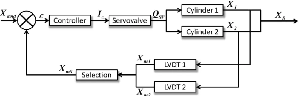
The system is composed of four equipments: the DECU, or controller, the servovalve and two cylinders with encompassed LVDT sensors. The regulated variable is the real selected position of the cylinder 𝑋𝑆 equal to the mean of 𝑋1 and 𝑋2 respectively real positions of cylinders 1 and 2. The VSV loop scheme is given in Fig. 7, where 𝑋𝑑𝑚𝑑 is the position demand, 𝑋𝑚1 and 𝑋𝑚2 the measured position from respectively LVDT1 and LVDT2, 𝑋𝑚𝑆 the selected measured position, 𝜀 the error, 𝐼𝑐 the control current, and 𝑄𝑆𝑉 the outlet flow from the servovalve.
System’s Equipments 6.1.3.
DECU: The DECU performs two main functions. The first one is to regulate the position of the actuators via a feedback mechanism of type Proportional-Integral-Derivative (PID) with variable gains. The second one is to calculate the most probable value of the measured position 𝑋𝑚𝑆 from 𝑋𝑚1 and 𝑋𝑚2. In this paper, we suppose that this selected value is the mean of the two measured values. The sampling period or Real Time Clock (RTC) of the DECU is
equal to 0.015s.
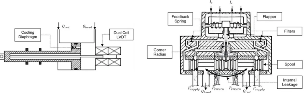
Actuators: The translation of the VSV actuator rod induces the movement of the VSV kinematic that is attached to the individual stator vanes. The two cylinders’ rods are linked by a flexible connection with known stiffness 𝐾. The VSV Actuators are fuel driven actuators. In order to prevent the fuel from coking because of overheating, a cooling diaphragm links the two chambers (see Fig. 8).
LVDTs: Each of the two actuators contains a single dual coil Linear Variable Differential Transformer (LVDT) sensor which allows the close loop control (see Fig. 8).
Servovalve: The servovalve is of type flapper-nozzle. Fig. 8 shows the architecture of this type of servovalve. The pressure difference ∆𝑃 between supply and return ports depends on the rotation speed of the engine 𝑁2. The servovalve feeds the two cylinders. The null current is the current for which the servovalve is in an equilibrium state, i.e. when the flapper is centered.
6.2. System Analysis
Failures, Faults and Degradation Modes 6.2.1.
Failures: From the risk analysis method results, we were able to determine the potential failure of the system. The subsystem VSV is subjected to one failure which is the loss of controllability of the loop. In order to prevent the system from reaching this failure, some faults were defined by engineers:
Faults:
o Position fault: when the absolute value of the error 𝜀 is higher than 2.9mm during 10 RTC. o Position gap fault: when the position gap between 𝑋𝑚1 and 𝑋𝑚2 is greater than 3.5mm.
Both are no dispatch faults so their associated degradation modes are high hazard degradation modes:
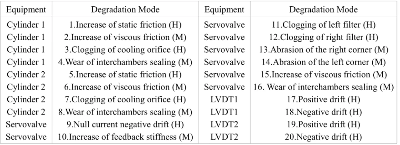
Degradation modes: the list of degradation modes was determined thanks to a combination of expert knowledge and good studies on servovalve degradation modes which can be found in [13] and [14]. Some degradation modes were also added to the list after a physical analysis of the model. The list of both hazardous and marginal degradation modes is given in Table 1 were “(H)” means hazardous and “(M)” means marginal degradation modes.
Table 1: List of the VSV loop’s degradation modes
Equipment Degradation Mode Equipment Degradation Mode
Cylinder 1 Cylinder 1 Cylinder 1 Cylinder 1 Cylinder 2 Cylinder 2 Cylinder 2 Cylinder 2 Servovalve Servovalve
1.Increase of static friction (H) 2.Increase of viscous friction (M) 3.Clogging of cooling orifice (H) 4.Wear of interchambers sealing (M)
5.Increase of static friction (H) 6.Increase of viscous friction (M) 7.Clogging of cooling orifice (H) 8.Wear of interchambers sealing (M)
9.Null current negative drift (H) 10.Increase of feedback stiffness (M)
Servovalve Servovalve Servovalve Servovalve Servovalve Servovalve LVDT1 LVDT1 LVDT2 LVDT2
11.Clogging of left filter (H) 12.Clogging of right filter (H) 13.Abrasion of the right corner (M)
14.Abrasion of the left corner (M) 15.Increase of viscous friction (M) 16. Wear of interchambers sealing (M)
17.Positive drift (H) 18.Negative drift (H) 19.Positive drift (H) 20.Negative drift (H) Uncertainties Management 6.2.2.
Thanks to both analysis of data from other engines and expert knowledge, the list of context and epistemic random parameters was established. The following Table 2 gives, for each parameter, its type (C for context and E for epistemic), its abbreviation and its uncertainty quantification under the form of a PDF where 𝒩(𝜇, 𝜎) defines a normal distribution of mean 𝜇 and standard deviation 𝜎 and 𝒰(𝑎, 𝑏) defines a uniform distribution between 𝑎 and 𝑏. The real values cannot be given here because matters of confidentiality.
Table 2: List of the VSV loop’s context and epistemic parameters and their uncertainties
Parameter Uncertainties Parameter Uncertainties
C: Fuel temperature 𝑇𝑓 𝒩(𝜇, 𝜎) E: Diameter rod cyl2 𝐷𝑟2 𝒰(𝑎, 𝑏)
E: Diameter piston cyl1 𝐷𝑝1 𝒰(𝑎, 𝑏) E: Mass cyl2 𝑀2 𝒰(𝑎, 𝑏)
E: Diameter rod cyl1 𝐷𝑟1 𝒰(𝑎, 𝑏) E: Chamber length cyl2 𝐶ℎ𝑙2 𝒰(𝑎, 𝑏) E: Mass cyl1 𝑀1 𝒰(𝑎, 𝑏) E: Diameter piston servo 𝐷𝑝𝑠 𝒰(𝑎, 𝑏) E: Chamber length cyl1 𝐶ℎ𝑙1 𝒰(𝑎, 𝑏) E: Diameter rod servo 𝐷𝑟𝑠 𝒰(𝑎, 𝑏) E: Diameter piston cyl2 𝐷𝑝2 𝒰(𝑎, 𝑏) E: Mass spool servo 𝑀𝑠 𝒰(𝑎, 𝑏)
Health Indicators 6.2.3.
In order to define relevant HI for monitoring the VSV loop, the acceptance test procedures were a good source of inspiration. For the servovalve, ATP are based on the analysis of the flow gain curve, giving the servovalve outlet flow versus the control current. This flow gain curve being a good indicator of the servovalve behavior’s conformity, the first idea is to monitor this flow gain. This operation can effectively be done during maintenance check-ups but it requires important offline instrumentation to isolate the servovalve and measure the flow. However, when the VSV loop is online, not only the servovalve is part of a subsystem but also it is not equipped with a flowmeter so we need to find indirect monitoring means. The proposed solution, which was the subject of a patent [15], is to use the selected cylinder’s velocity as an image of the servovalve outlet flow to compute the velocity gain curve. Because of the hysteresis, the raw curve has a
large dispersion so we use a smoothing algorithm in order to obtain an exploitable curve, as shown in Fig. 9. Then, we define 10 HI from characteristics extracted from this curve, listed in Table 3.
Table 3: List of Health Indicators from the velocity gain curve
HI Definition HI Definition 𝐶𝐸𝑞𝑢 𝑌𝑛𝑢𝑙𝑙 𝑌𝑜𝑣𝑒𝑟𝑙𝑎𝑝 𝑆𝑙𝑝𝐿𝑒𝑓𝑡 𝑆𝑙𝑝𝑅𝑖𝑔ℎ𝑡
Equilibrium point abscissa Null point abscissa
Length of the low gain part projected on the ordinate axis
Slope of the left high gain regression Slope of the right high gain
regression 𝑋𝑛𝑢𝑙𝑙 𝑋𝑜𝑣𝑒𝑟𝑙𝑎𝑝 𝑆𝑐𝑎𝑙𝑒 𝑆𝑙𝑝𝑁𝑢𝑙𝑙 𝐻𝑦𝑠𝑡0
Null point abscissa
Length of the low gain part projected on the abscissa axis
Difference between the highest and the lowest value of control current
Slope of the low gain regression Standard deviation of null velocity
points
6.3. Simulations
System’s modeling 6.3.1.
The physics-based modeling of the VSV loop is performed on the commercial software AMESim© [16]. AMESim is a proven tool for modeling and analysis of multi-domain systems. Models are described by nonlinear analytical equations that represent the system’s hydraulic, pneumatic, thermal, electric or mechanical behavior. To create a model, we use a set of libraries containing different components and subsystems which have been validated by different engineering domains. The main advantage of this type of simulation is that it allows capturing the system behavior before detailed CAD geometry is available. Hence, it is particularly useful in the upstream development stages of a system.
Uncertainties Propagation 6.3.2.
The propagation of uncertainties is performed via Monte-Carlo simulations. The Monte-Carlo samples are generated in Matlab-Simulink and a cosimulation interface sends the values of parameters to AMESim before finally retrieving the HI values in return. The main advantage of using this cosimulation scheme is that HI are available in the Matlab environment so both classical toolbox functions and specific processing script can be used directly.
6.4. Health Indicators’ Validation
Specifications 6.4.1.
For this application, the specifications given by customers were the following ones: 𝑇𝑃𝑆𝑃𝐸𝐶 = 0.9 and 𝐹𝑃𝑆𝑃𝐸𝐶 = 0.01
𝐷𝐻% = 90% ; 𝐼𝐻% = 80% ; 𝑃𝐻% = 90%
𝐿𝑈% = 100%
First Performance Metrics Computation 6.4.2.
This first computation of the detectability matrix (see the ten first columns of the detectability matrix in Fig. 10) shows that the four last lines have no column were the value of the detectability index is equal to 1. It means that those four degradation modes are not detectable. Because they are hazardous degradation modes, it means that specifications will not be meet so some complementary HI are needed.
Addition of new Health Indicators 6.4.3.
As explained before, the VSV loop contains two LVDT sensors measuring the position of cylinder. Ideally, both measures should be identical if the cylinders were strictly the same of if the value of 𝐾 (stiffness of the bound between cylinders) was high. Yet in reality, the cylinders are
Fig. 10: NKPI for the set of health indicators: detectability matrix (left),
different from each other and the complexity of the kinematic results in a low 𝐾. Moreover, the failure modes analysis revealed that some hazardous degradation modes can induce a drift of LVDT values. From this observation, we have defined 8 HI listed in Table 4:
Table 4: List of additional Health Indicators from the position profile
HI Definition HI Definition 𝑚𝑎𝑥𝑋1 𝑚𝑖𝑛𝑋1 𝑚𝑎𝑥𝐺𝑎𝑝𝑋 𝑚𝑖𝑛𝐺𝑎𝑝𝑋 LVDT1 max value LVDT1 min value Maximum gap between LVDT1’s
and LVDT2’s position values Minimun gap between LVDT1’s and
LVDT2’s position values 𝑚𝑎𝑥𝑋2 𝑚𝑖𝑛𝑋2 𝑚𝑒𝑎𝑛𝐺𝑎𝑝𝑋 𝑠𝑡𝑑𝐺𝑎𝑝𝑋 LVDT2 max value LVDT2 min value Mean gap between LVDT1’s and
LVDT2’s position values Standard deviation of the gap between LVDT1’s and LVDT2’s Second Performance Metrics Computation
6.4.4.
The second computation of the detectability matrix (see Fig. 10) shows that all the hazardous degradation modes are detectable. The identificability matrix is not shown but it would reveal that all the hazardous degradation modes are detectable. Eventually, the localizability matrix traduces that the five LRU are localizable and the prognosticability matrix shows that all the hazardous degradation modes are prognosticable.
In the end, the computation of NKPI highlights that all the specifications for health indicators are validated: for 𝑇𝑃𝑆𝑃𝐸𝐶 = 0.9 and 𝐹𝑃𝑆𝑃𝐸𝐶 = 0.01, 𝐷𝐻% = 100%, 𝐼𝐻% = 100%, 𝐿𝑈% = 100% and 𝑃𝐻% = 100%. It means that the selected set of HI is validated with respect to specifications.
7. Conclusion
In this paper, the issue of dependability management in aircraft engines manufacturing industry is addressed through the following central problem: what are the solutions to improve availability to reduce maintenance costs. Over the last decade, one solution seems to impose itself: Prognostics and Health Management which is becoming increasingly important within the aeronautical field. However, despite its potential, PHM is still considered as a marginal process in the industry with neither formalized development process nor real validation tools.
In the course of this paper, the authors have proposed a method to improve the selection and validation of health indicators for PHM in the early stages of the host system’s development process. The first section have introduced the PHM framework through a set of definition of threats, collecting vectors and processing means. The specificities of the PHM architecture in aircraft engines were also presented with focus on the collecting station. The selection of HI is based on the knowledge about the host system’s architecture, risk analysis methods, equipment specifications and acceptance test procedures. The validation is based on performance metrics called numerical key performance indicators defined from ROC curves. The computation of NKPI needs some distributions of HI obtained via a combination of physics-based modeling and uncertainties propagation.
In the last section, the method is applied to the monitoring of the VSV loop in aircraft engines. After having determined the list of degradation modes and fault, the first selection of health indicators was based on the construction of the velocity gain curve, inspired from acceptance test
procedures. The set of HI has unfortunately proved itself insufficient to detect all the hazardous degradation modes so some other HI were added to the set in order to improve the performance. This second set was validated because NKPI indicated that it allowed detectability, identificability and prognosticability of all the degradation modes and localizability of all the LRU.
Thus, although not based on complex theory, the method showed very promising results which were welcomed by the industry because of their physical based aspect. The computation of NKPI allowed to support the presentation of the monitoring logic with some quantifiable aspects so that the host system designers have accepted to implement the collecting of these HI into future engines. This approach could become systematic in upcoming years because of the following observation: for aircraft engines manufacturer, the more than likely generalization of flight hour contract will make them responsible for unavailability costs whereas they currently make profit thanks to maintenance. Thus, this switch of business model will turn PHM into a strategic and unavoidable selling asset.
In the end, the main future prospects are: first, to develop a method to recalibrate the model with the first operational measured data in order to validate the modeling part. Then, to use surrogate modeling to reduce the simulation costs of the uncertainties propagation and finally, the ultimate objective is to apply the method to the entire aircraft engine.
References
[1] J.-C. Laprie, «Dependable Computing and Fault Tolerance: Concepts and terminology,» chez
Proceedings of the 15th IEEE International Symposium on Fault-Tolerant, 1985.
[2] K. Diamanti et C. Soutis, «Structural health monitoring techniques for aircraft composite structures,» Progress in Aerospace Sciences, vol. 46, n° %18, pp. 342-352, November 2010. [3] J. Sheppard, M. Kaufman and T. Wilmer, "IEEE Standards for Prognostics and Health
Management," Aerospace and Electronic Systems Magazine, vol. 24, no. 9, p. 34–41, 2009. [4] «OSA-CBM Website,» [En ligne]. Available: http://www.osacbm.org/.
[5] J. Chen et R. J. Patton, «Review of parity space approaches to fault diagnosis for aerospace systems,» Journal of Guidance, Control, and Dynamics, vol. 17, n° %12, 2012.
[6] A. Patterson-Hine, G. Biswas, G. Aaseng, S. Narasimhan and K. Pattipati, "A Review of Diagnostic Techniques for ISHM Applications," vol. 1st Integrated Systems Health Engineering and Management Forum, 2005.
[7] M. Roemer, C. S. Byington, G. J. Kacprzynski et G. Vachtsevanos, «An overview of selected prognostic technologies with reference to an integrated PHM architecture,» 2007.
[8] T. Fawcett, An introduction to ROC analysis, 2164 Staunton Court, Palo Alto: Institute for the Study of Learning and Expertise, 2005.
[9] T. D. Wickens, Elementary Signal Detection Theory, N. Y. O. U. Press, Éd., 2002. (ISBN 0-19-509250-3).
[10] E. De Rocquigny, N. Devictor, S. Tarantola, F. Mangeant, C. Schwob, R. Bolado-Lavin, J. R. Massé, P. Limbourg, W. Kanning and P. Van Gelder, Uncertainty in industrial practice: A guide to quantitative uncertainty management, Wiley, 2007.
[11] N. Metropolis et S. Ulam, «The Monte Carlo Method,» Journal of the American Statistical
Association, vol. 44, n° %1247, pp. 335-341, 1949.
[12] B. Lamoureux, N. Mechbal et J. R. Massé, «Selection and Validation of Health Indicators in Prognostics and Health Management System Design,» chez Proceedings of Systol'13, Nice, 2013. [13] L. Borello, M. D. Vedova, G. Jacazio et M. Sorli, «A Prognostic Model for Electrohydraulic
Servovalves,» Annual Conference of the Prognostics and Health Management Society, 2009. [14] K. Zhang, Y. Jinyong, J. Tongmin, Y. Xizhong et Y. Xiaobo, «Degradation Behavior Analysis of
Electro-Hydraulic Servo Valve under Erosion Wear,» chez Proceedings of IEEE International
Conference on Prognostics and Health Management, Washington D.C., 2013.
[15] J. R. Massé, B. Lamoureux, C. Aurousseau, R. Deldalle, P. Michel, X. Flandrois et A. Sif, «METHOD AND DEVICE FOR MONITORING A FEEDBACK LOOP OF A VARIABLE-GEOMETRY ACTUATOR SYSTEM OF A JET ENGINE». Geneva, Switzerland Brevet World Intellectual Property Organization Patent No. 2012052696, 27 april 2012.