Science Arts & Métiers (SAM)
is an open access repository that collects the work of Arts et Métiers Institute of Technology researchers and makes it freely available over the web where possible.
This is an author-deposited version published in: https://sam.ensam.eu
Handle ID: .http://hdl.handle.net/10985/20121
To cite this version :
Meryeme TOTO JAMIL, Abdelkader BENABOU, Stéphane CLÉNET, Sylvain SHIHAB, Laure LE BELLU ARBENZ, Jean-Claude MIPO - Magneto-thermal characterization of bulk forged magnetic steel used in claw pole machine - Journal of Magnetism and Magnetic Materials - Vol. 502, p.166526 - 2020
Any correspondence concerning this service should be sent to the repository Administrator : archiveouverte@ensam.eu
1
Magneto-thermal characterization of bulk forged magnetic steel used in
claw pole machine
Meryeme TOTO JAMIL1,2, Abdelkader BENABOU1,*, Stéphane CLENET1, Sylvain
SHIHAB1, Laure LE BELLU ARBENZ2, Jean-Claude MIPO2
1Univ. Lille, Arts et Metiers ParisTech, Centrale Lille, HEI, EA 2697 - L2EP -Laboratoire
d’Electrotechnique et d’Electronique de Puissance, F-59000 Lille, France
2Valeo Powertrain Systems, 2 Rue André Charles Boulle, 94046 Créteil Cedex, France *Corresponding author e-mail: Abdelkader.Benabou@univ-lille.fr, Phone: +33 (0) 3 62 26
82 15
Abstract
During the operation of Claw Pole (CP) machines, and for some operating loads, the magnetic core temperature can reach 180°C in some hot spots. As a consequence, the core electromagnetic properties may considerably change, impacting the machine performances. In such a case, a deep knowledge of the electromagnetic behavior as a function of the temperature is required.
In this paper, we present a dedicated study of the CP rotor made from a forged magnetic steel. In fact, the CP magnetic properties heterogeneity and the claw shape made it necessary to extract specific samples that are characterized with a miniaturized Single Sheet Tester (SST). To that end, this work proposes a specific methodology to characterize the electromagnetic properties of the CP rotor material as a function of the temperature in order to better predict the machine electrical performances, especially regarding the iron losses.
Keywords: Temperature dependence; magnetic properties; magneto-thermal
characterization; electrical conductivity.
1. Introduction
Magnetic materials are at the heart of the energy conversion in electrical machines. Their electric and magnetic properties are strongly related to the machine performances and energy efficiency. In order to study and to simulate the electrical machine under its operating conditions, the material electromagnetic behavior should be well known and well characterized not only at room temperature but also at the machine operating temperatures. In fact, during
2
the machine operation, in some hot spots, the magnetic core temperature may reach up to 180°C [1]. As a consequence, the magnetic core properties may considerably change, as for the electrical conductivity to which eddy current losses are directly linked [2]–[5]. Thus, when a massive magnetic core is involved, especially the CP rotor, the temperature effects must be carefully considered in the energy conversion process. Therefore, to predict accurately the machine performances, it is necessary to perform both thermal and electromagnetic analyses, starting by characterizing the temperature dependence of the core electromagnetic properties.
In the standard experimental approaches for magnetic measurements, the characterization techniques are rarely adapted to temperatures up to 200°C. In different works, the authors designed specific magneto-thermal characterization devices based on specific needs. Some of them employed the ring core method [3], [6], [7] while few others used an adapted Single Sheet Tester (SST) [5], [8] or even rarely the Epstein frame [9]. However, these techniques are limited to steel sheets. Likewise, they are not adapted to forged heterogeneous bulk core as it is the case for the CP of automotive alternator.
Consequently, the CP requires a specific methodology. Its magnetic core is a massive forged piece with a complex shape through which the magnetic flux has three dimensional trajectories. Also, because of the manufacturing process the CP magnetic properties turn out to be strongly heterogeneous [10]. They vary not only in a given CP but also from one to another. For these reasons, a specific testing device was developed in order to characterize bulk parallelepiped samples extracted from different regions of the CP [11]. However, this characterization device is limited to ambient temperature measurements.
In this paper, a specific methodology and an experimental set-up are proposed to characterize the electromagnetic properties of the CP as a function of the temperature up to 200°C. The temperature dependence of the electromagnetic properties, especially the B-H curve, iron losses and electrical conductivity, are studied. First, the experimental setup is described. Then, the experimental results of the temperature effect on the electrical conductivity and magnetic properties are presented and discussed. Finally, the link between the electrical conductivity and the dynamic losses dependence with temperature is considered.
2. Experimental setup
A magneto-thermal characterization device has been developed for this specific study. The illustration of the device is given in Figure 1. It consists in a miniaturized SST able to work from room temperature and up to 200°C. The supporting frame is made from PolyEther Ether Ketone (PEEK) which exhibits a low coefficient of thermal expansion (10-5.K-1) up to 260°C.
3
As presented in [11] and illustrated in Figure 1, the setup is composed of one yoke, the primary coil to create magnetic field, a secondary coil to measure the polarization J and two high precision Hall sensors to measure the magnetic field. These latter include temperature compensation up to 200°C, with very small linearity error (typically 0,1 % up to 1,5 T). The measurement device has been validated by numerical 2D / 3D simulations as detailed in [11]. Furthermore, the mini-SST measurements were compared, at room temperature, with those made on a standardized SST, and a very good agreement was observed between measurements made on both devices. For instance, to reach a magnetic induction of 1.5T, the relative gap between the magnetic fields, measured with the mini-SST and standard SST, is about 1.15%. Likewise, for the same level of magnetic flux density, the gap is equal to 2.3% for the specific losses. The electrical conductivity is measured at different temperatures using the four probes methods and applying a geometry correction factor as explained in [11], [12].
For both the electrical and magnetic devices, the used cables and copper wires can support temperatures above 200°C. In order to control the temperature of the environment, the device is placed in a drying and heating chamber (Binder, model M53) with a heating capability ranging from 5°C above the room temperature to 300°C. The temperature chamber is also equipped with forced convection and adjustable fan speed functions that allow to have a homogeneous temperature with less than 2°C of variation within the heated volume. Moreover, in addition to the temperature sensor in the heating chamber, a thermocouple is placed on the sample to check its temperature and ensure the thermal equilibrium in the heating chamber.
The experiments were carried out on two bulk parallelepiped samples with dimensions 35 mm x 10 mm x 1 mm. The samples were extracted by Wire Electrical Discharge Machining (WEDM) in two different locations of a CP made from SAE1006 steel. The WEDM process has been chosen because of its low impact on the electromagnetic properties.
4
Figure 1. Magneto-thermal characterization device
3. Measurement results and discussion
3.1. Electrical conductivity
The experimental protocol for the measurement of the electrical conductivity consists in placing the sample in the heating chamber and increasing the temperature by steps of 25°C, starting from the room temperature (25°C) and up to 200°C. After each step, once the thermal steady state is reached, the electrical measurement is performed. As mentioned in the previous section, the electrical conductivity is deduced from the following equation:
𝜎 = 𝐼ℓ
𝑉𝑆𝐹, (Eq 1)
where 𝜎 is the electrical conductivity, 𝐼 current, ℓ the distance between the voltage probes, 𝑉 the measured voltage, 𝑆 the section of the sample and 𝐹 is a correction factor that accounts for the geometry of the sample [11].
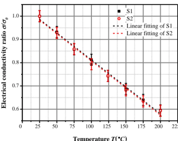
The results of the electrical measurements of both considered samples “S1 and S2” are reported in Figure 2. As expected, a linear relationship is observed between the electrical conductivity and the temperature, which can be written:
𝜎(𝑇) = −0,014 (𝑇 − T0) + σ0 (Eq 2)
Primary magnetizing winding (75 turns)
Hall Effect sensors Sample
Yoke
Secondary winding (47 turns)
5
where 𝜎(𝑇) is the electrical conductivity at the temperature T (°C) and σ0 is the electrical conductivity at room temperature T0 (25°C). Thus, for temperatures between 25°C and 200°C, the electrical conductivity decreases with a rate of 0.23% /°C. This decrease of the electrical conductivity was expected. In fact, due to thermal agitation, the mobility of the charge carrier decreases and, as a result, the ability of the material to conduct electrical current is reduced [2]. However, an accurate determination of the rate can only be done experimentally.
0 25 50 75 100 125 150 175 200 225 0.6 0.7 0.8 0.9 1.0 Elec tr ic al con du ct ivity ratio / 0 Temperature T(°C) S1 S2 Linear fitting of S1 Linear fitting of S2
Figure 2. The electrical conductivity ratio 𝜎/𝜎0 as a function of the temperature (with 𝜎0 the electrical conductivity measured at 25°C)
3.2. Magnetic properties
In the same way, as for the electrical conductivity, the experimental protocol consists in placing the whole device (supporting frame + sample) inside the temperature chamber and performing the measurement once the thermal steady state is reached. The considered temperatures for the magnetic measurements are the room temperature (25°C) and by 50°C steps starting from 50°C and up to 200°C. The measurements were systematically carried out on both the samples to ensure the reproducibility of the observations. And, as expected, both samples showed similar behaviors. Thereafter, only the results of the measurement made on sample S1 are presented.
In Figure 3, the hysteresis loops are illustrated for the considered temperatures and for 1.5 T peak magnetic induction at 50Hz frequency.
6 -3000 -2000 -1000 0 1000 2000 3000 -2.0 -1.5 -1.0 -0.5 0.0 0.5 1.0 1.5 2.0 2000 2200 2400 1.45 1.50 1.55 B[T] B(T) H(A/m) 25°C 50°C 100°C 150°C 200°C
Figure 3. Hysteresis loops of the CP sample characterized at 1.5T/50 Hz at different temperatures
Comparing the hysteresis loops measured at different temperatures, a contraction of the loop area is clearly observed when the temperature increases. This is associated to the decrease of the coercive field, which represents the magnetic field required to demagnetize the sample, with increasing temperature [9]. Besides, as the temperature increases, thermal energy tends more and more to break the spontaneous alignment of atoms. As a result, the magnetization and the susceptibility decrease [13]. In this range of temperature, this behavior is barely noticeable, for this kind of material. In fact, in the saturation zone presented in Erreur ! Source du renvoi introuvable., the saturation induction is reduced by 3%. The same tendency of temperature dependence was observed on FeSi sheets in [3], [9].
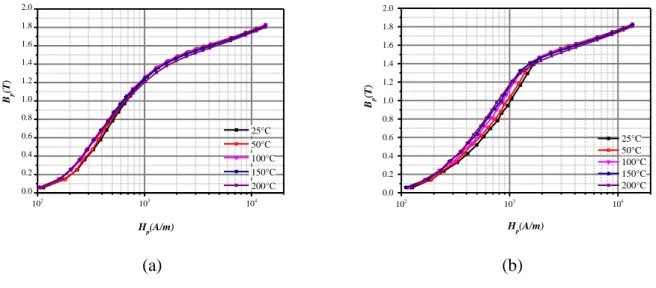
The normal magnetization curve, obtained from the tips Bp-Hp of increasing induction level of minor hysteresis loops, is presented in Figure 4Erreur ! Source du renvoi introuvable. for different temperatures. It is found that, as temperature increases, the magnetic flux density increases for low magnetic fields but decreases slightly at higher magnetic fields above the knee region. This result may be explained by the combination of two effects. The first is the temperature dependence of the saturation magnetization which diminishes with the temperature, and is more pronounced at high magnetic field. The second is related to the dynamic effects which are more visible at low magnetic field. In fact, the total magnetic field H is the sum of the static field 𝐻𝑠𝑡𝑎𝑡 (frequency-independent) and the dynamic field 𝐻𝑑𝑦𝑛due to eddy-currents. When the temperature increases, the eddy currents effect is reduced due to the decrease of the electrical conductivity as shown in the previous section. Consequently, the
7
dynamic field decreases as well with the temperature. Therefore, at low magnetic field, to reach a given magnetic flux density level, the total required magnetic field is less important when the temperature increases. This effect is more noticeable at high frequency measurement (Figure 4.(b)) when the dynamic effects are more pronounced. However, compared to the variation due to the frequency, the temperature effect on the magnetization curves is less significant. The same behavior was observed in [14].
102 103 104 0.0 0.2 0.4 0.6 0.8 1.0 1.2 1.4 1.6 1.8 2.0 Bp (T) H p(A/m) 25°C 50°C 100°C 150°C 200°C 102 103 104 0.0 0.2 0.4 0.6 0.8 1.0 1.2 1.4 1.6 1.8 2.0 Bp (T) H p(A/m) 25°C 50°C 100°C 150°C 200°C (a) (b)
Figure 4. B-H curves (log-scale for H-field) of the sample characterized at different temperatures, (a) at 50 Hz and (b) at 200 Hz.
The previous observations can be emphasized by plotting the relative permeability calculated by (Eq 3), µ𝑟 = 1 µ0∗ 𝐵𝑝 𝐻𝑝 (Eq 3)
where µ0 is vacuum magnetic permeability and (Hp, Bp) are the tips of minor loops. The effect of temperature on the relative permeability is reported in Figure 5. It is observed that, when the temperature increases, the permeability increases at low magnetic flux density whereas it decreases at high magnetic flux density. This is associated to the temperature dependence of the material susceptibility and eddy current effects as noted previously on the magnetization curves.
It should be noted that the increase of the magnetic permeability with temperature at low flux density may also be explained by the Hopkinson effect as shown in [3]. This effect is noticeable at high temperature when approaching the Curie temperature. Nevertheless,
8
regarding the considered temperature range in the present study (below 200°C) and the SAE 1006 material (TCurie=770°C) this effect is barely pronounced.
0.0 0.2 0.4 0.6 0.8 1.0 1.2 1.4 1.6 1.8 2.0 0 200 400 600 800 1000 1200 1400 1600 r Bp(T) 25°C 50°C 100°C 150°C 200°C
Figure 5. Relative permeability of the CP sample characterized at 50 Hz at different temperatures
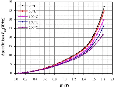
Regarding the iron losses, the effect of the temperature is more significant as we can see in Figure 6. It gives the evolution of the total losses in function of the magnetic flux density for different temperatures. The main observation is a significant decrease of the total iron losses when the temperature increases.
0.0 0.2 0.4 0.6 0.8 1.0 1.2 1.4 1.6 1.8 2.0 0 5 10 15 20 25 30 35 40 Specif ic l oss Ptot (W/ kg) Bp(T) 25°C 50°C 100°C 150°C 200°C
9
To further investigate the total losses 𝑃𝑡𝑜𝑡 dependence with temperature, a loss separation is performed. The losses are decomposed into the hysteresis 𝑃ℎ𝑦𝑠 and dynamic 𝑃𝑑𝑦𝑛 contributions such as:
𝑃𝑡𝑜𝑡 = 𝑃ℎ𝑦𝑠 + 𝑃𝑑𝑦𝑛 (Eq 4)
To determine the hysteresis loss component, energy losses (𝑃/𝑓) measurements at five different frequencies, respectively 1Hz, 5Hz, 20Hz, 50Hz, 100Hz and 200Hz, were used. The hysteresis losses were calculated by extrapolating these measurements to zero frequency. The dynamic losses were then obtained after subtracting hysteresis losses from the total losses for each frequency. Note that the dynamic loss contribution includes the classical losses and the excess losses as defined in the Bertotti’s loss decomposition approach.
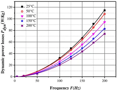
The evolution of the dynamic losses as a function of frequency, for 1.5 T peak magnetic induction, is presented for different temperatures in Figure 7. The dynamic losses exhibit an evolution quasi-proportional to the square of the frequency, as it is the case for the classical losses due to macroscopic eddy currents [15]. It confirms that, in the following, the dynamic losses could be assimilated to the classical losses.
0 50 100 150 200 0 20 40 60 80 100 120 Dy na mic pow er losse s Pdyn ( W/Kg ) Frequency F(Hz) 25°C 50°C 100°C 150°C 200°C
Figure 7 : Dynamic power losses as a function of frequency at 1.5T for different temperatures.
In addition, to describe and to quantify the relative variation with temperature of each of the hysteresis and dynamic losses, the losses were normalized respectively to 𝑃ℎ𝑦𝑠(25°𝐶) and
10 𝑃ℎ𝑦𝑠𝑛 = 𝑃ℎ𝑦𝑠(𝑇°) 𝑃ℎ𝑦𝑠(25°𝐶), 𝑃𝑑𝑦𝑛𝑛 = 𝑃𝑑𝑦𝑛(𝑇°) 𝑃𝑑𝑦𝑛(25°𝐶) (Eq 5)
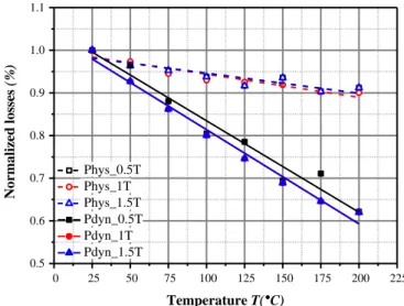
Figure 8 illustrates the temperature dependence of these loss components at 0.5T, 1T and 1.5T peak induction levels. It is noted that the hysteresis losses decrease slightly with temperature (0.07% /°C) while the dynamic losses decrease more significantly. The noted behavior is the same for different peak induction levels. This modification of the dynamic losses is obviously explained by the variation of the eddy current losses which are directly linked to the electrical conductivity.
0 25 50 75 100 125 150 175 200 225 0.5 0.6 0.7 0.8 0.9 1.0 1.1 Phys_0.5T Phys_1T Phys_1.5T Pdyn_0.5T Pdyn_1T Pdyn_1.5T No rmaliz ed losse s (%) Temperature T(°C)
Figure 8: Normalized hysteresis and dynamic losses as a function of temperature measured at 0.5T, 1T and 1.5T.
Theory predicts that the dynamic losses are a linear function of the electrical conductivity [15] and we have shown experimentally that the electrical conductivity is a linear function of the temperature. Consequently, we can expect the dynamic losses to exhibit a linear behavior in function of the temperature with a coefficient of variation close to the one of the electrical conductivity. The experimental results presented in Figure 8 confirm that the dynamic losses are a linear function of the temperature and that the coefficient equal to 0.21%/°C is close to the one of the electrical conductivity which is equal to 0.23%/°C.
11
In this paper a methodology for the characterization of the electromagnetic properties of bulk materials under different temperatures up to 200°C was proposed. The characterization results showed a clear temperature dependence of the electromagnetic properties. The coercive field, the saturation magnetization and the material permeability decrease when the temperature increases. Also, for the considered material, the electrical conductivity decreases in a linear way with temperature. Consequently, the eddy currents are reduced and thus the total losses decrease. The temperature affects also the magnetization curve which was found to be more influenced by the frequency and varies slightly with the temperature. Finally, from the separation of the losses, it has been concluded that the variation of the dynamic losses as a function of temperature is close to the one of the electrical conductivity. Yet, this result can further be used in the development of a loss prediction model using, on the one hand, temperature dependent electrical conductivity measurements and, on the other hand, iron loss measurements at room temperature only. In the context of electrical machine applications, the effect of the operating temperature on the magnetic core will be further accounted for in an easier way to provide a realistic simulation of the machine performance.
References
[1] S. Brisset, M. Hecquet, and P. Brochet, “Thermal modelling of a car alternator with claw poles using 2D finite element software,” COMPEL - Int. J. Comput. Math. Electr.
Electron. Eng., vol. 20, no. 1, pp. 205–215, Jan. 2001
[2] Sun Yafei, Niu Dongjie, and Sun Jing, “Temperature and carbon content dependence of electrical resistivity of carbon steel,” in 2009 4th IEEE Conference on Industrial
Electronics and Applications, pp. 368–372, 2009.
[3] N. Takahashi, M. Morishita, D. Miyagi, and M. Nakano, “Examination of Magnetic Properties of Magnetic Materials at High Temperature Using a Ring Specimen,” IEEE
Trans. Magn., vol. 46, no. 2, pp. 548–551, Feb. 2010.
[4] M. MacLaren, “The Effect of Temperature upon the Hysteresis Loss in Sheet Steel,”
Trans. Am. Inst. Electr. Eng., vol. XXXI, no. 2, pp. 2025–2035, Jun. 1912.
[5] M. Nakaoka, A. Fukuma, H. Nakaya, D. Miyagi, M. Nakano, and N. Takahashi, “Examination of Temperature Characteristics of Magnetic Properties Using a Single Sheet Tester,” IEEJ Trans. Fundam. Mater., vol. 125, no. 1, pp. 63–68, 2005.
[6] N. Takahashi, M. Morishita, D. Miyagi, and M. Nakano, “Comparison of Magnetic Properties of Magnetic Materials at High Temperature,” IEEE Trans. Magn., vol. 47, no. 10, pp. 4352–4355, Oct. 2011.
[7] A. T. Bui, “Caractérisation et modélisation du comportement des matériaux magnétiques doux sous contrainte thermique,” thesis, Lyon 1, 2011.
[8] D. Chen, L. Fang, B. Kwon, and B. Bai, “Measurement research on magnetic properties of electrical sheet steel under different temperature, harmonic and dc bias,” AIP Adv., vol. 7, no. 5, p. 056682, May 2017.
[9] C. W. Chen, “Temperature Dependence of Magnetic Properties of Silicon‐Iron,” J. Appl.
12
[10] M. Borsenberger, “Contribution to the identification of the interaction between process parameters and functional properties of work pieces: Application to forging and to electromagnetic properties of alternator claw poles,” thesis, Paris, ENSAM, 2018. [11] M. Jamil, A. Benabou, S. Clénet, L. Arbenz, and J.-C. Mipo, “Development and
validation of an electrical and magnetic characterization device for massive parallelepiped specimen,” Int. J. Appl. Electromagn. Mech., pp. S1–S8, Jun. 2019.
[12] L. Arbenz, A. Benabou, S. Clenet, J. C. MIPO, and P. Faverolle, “Characterization of the local Electrical Properties of Electrical Machine Parts with non-Trivial Geometry,” Int. J.
Appl. Electromagn. Mech., vol. 48, no. 2&3, pp. 201–206, Jun. 2015.
[13] R. M. Bozorth, “Ferromagnetism,” Ferromagn. Richard M Bozorth Pp 992 ISBN
0-7803-1032-2 Wiley-VCH August 1993, Aug. 1993.
[14] J. Chen et al., “Influence of temperature on magnetic properties of silicon steel lamination,” AIP Adv., vol. 7, no. 5, p. 056113, May 2017.
[15] G. Bertotti, “General properties of power losses in soft ferromagnetic materials,” IEEE