Science Arts & Métiers (SAM)
is an open access repository that collects the work of Arts et Métiers Institute of Technology researchers and makes it freely available over the web where possible.
This is an author-deposited version published in: https://sam.ensam.eu Handle ID: .http://hdl.handle.net/10985/16935
To cite this version :
Guillaume MARTIN, Guillaume VERMOT DES ROCHES, Etienne BALMES, Thierry CHANCELIER - MDRE: an efficient expansion tool to perform model updating from squeal measurements - In: Eurobrake, Allemagne, 2019-05-23 - Eurobrake - 2019
Any correspondence concerning this service should be sent to the repository Administrator : archiveouverte@ensam.eu
MDRE: AN EFFICIENT EXPANSION TOOL TO PERFORM MODEL
UPDATING FROM SQUEAL MEASUREMENTS.
1Martin, Guillaume*, 1Vermot des Roches, Guillaume, 1,3Balmes, Etienne, 2Chancelier, Thierry
1 SDTools, France, 2 Chassis Brakes International, France, 3 PIMM, Arts et Metiers, CNRS, Hesam, France
e-mail: martin@sdtools.com
KEYWORDS – Expansion, model reduction, model updating, parametric study, test/model correlation
ABSTRACT
In brake FEM, model updating is often needed to improve the model accuracy and well describe problematic phenomena such as the squeal. To avoid performing a full model updating which is often time consuming, the use of the Minimum Dynamic Residual
Expansion method is proposed to help building the updating strategy. The procedure proposed in this paper is evaluated on a disc brake system, using experimental measurements and the nominal model as input data. From experimental squeal measurements, two shapes are extracted and expanded on the current model. The evaluation of the residual error of model shows areas where the model is wrong and guides through the definition of sensitive parameters which need to be updated. Once the model is parameterized, a model reduction strategy is proposed for further computations to be performed in a time compatible with industrial processes. A parametric study is then achieved: the expansion is computed for all the combinations of the chosen parameters. It is finally possible to navigate through the expansion results for all the parameters, evaluate the evolution of the model accuracy and extract the best combination which improves the model representability.
TECHNICAL PAPER
In brake models, it is difficult to be confident in the a priori relevance of some parameters. Model updating is thus often needed to properly represent the real system. In previous works, a full model updating method has been proposed [1,2]. To limit model bias in the updating result, the strategy was to update component alone first (geometry and material properties) and then to iteratively update isolated couplings in sub-models. This strategy is really relevant at the component level and for some couplings but can be time consuming (many
measurements are needed) and some parameters cannot be isolated in substructures (sliding contacts, shoes/back-plate, pad/bracket…)
A complementary updating procedure is thus needed. In [3], the Minimum Dynamic Residual Expansion (MDRE) [4,5], was first proposed to improve the interpretation of experimental shapes measured with low sensor density, typically with accelerometers. In presence of higher number of sensors, this expansion technique can also be used to highlight areas where model error exists [6,3]. It is proposed in this paper to go further with two steps: first with a model parameterization of the areas pointed out by the MDRE result and secondly by updating the parameters.
First, the system used as illustration is presented with a description of both numerical and experimental input data. Then, MDRE expansion theory is summarized and expansion results
on the test case are presented. Next, the implementation of the parametric model is developed and precisions are provided on how it can be used in the expansion process. Focus is also made on calculation times. Finally, results of the parametric study are shown and perspectives are provided to go further.
TEST CASE PRESENTATION
When dealing with squeal phenomenon, some parameters are really sensitive to braking conditions (especially the braking pressure) and need to be addressed to obtain a model representative enough to propose design countermeasures. Thus experimental data must be exploited to correlate and improve the model. Using in-squeal ODS correlation provides a good way of updating a brake model in specific operating conditions.
Two main techniques are available to perform the ODS measurements: using accelerometers which can be measured synchronously but have a low spatial resolution or using 3D Scanning Laser Doppler Vibrometer (3DSLDV) measurements which allow a higher spatial density but lead to sequential measurements. Using sequential measurements is a difficulty previously addressed in [3,6] because the squealing system cannot be considered as time invariant. Results from previous papers, with experiments on both drum and disc brakes, showed that the shapes associated with squeal instabilities are expected and actually found to be
dominated by the combination of two real modes. Despite frequency shifts, two real shapes dominate the response and have variations that are coherent with changes due to the wheel position.
Here a disc brake is used as illustration. The disc brake is measured in squealing conditions on test bench shown in Figure 1 left using the Polytec 3DSLDV PSV500. The test wireframe is constructed in two parts: one in the direct view to measure the disc, a part of the caliper and a part of the anchor bracket and one through the mirror to measure the remaining parts of the caliper and the anchor bracket. It is composed of 619 points, leading to 1857 measured channels (XYZ directions). The test wireframe is overlaid with the FEM in Figure 1 right.
Figure 1 : Test case. Left : disc-brake measured on test bench. Right : Measurement wireframe on top of the FEM.
To extract the two main shapes; three reference mono-axial accelerometers were used: one on the caliper, one on the anchor bracket and one on the arm. From sequential time
measurements, the procedure presented in [3,6] was used to extract two main real shapes around 4250Hz, where squeal occurs. The two main shapes are shown in Figure 2.
Figure 2 : Visualization of the two main shapes extracted from all the sequential time measurement with the previously developed method
The first shape shows mainly a deformation of the bracket. The second shape shows another deformation of the bracket with a deformation of the disc.
On the modelling side, the brake assembly is simulated with finite elements. All components are in contact friction-interaction. A steady-sliding state in brake actuation conditions is computed to obtain contact and friction statuses from which a tangent model is derived (linearization) for eigenvalue analysis. The model used in this study is a quality checked (mesh convergence, steady sliding state consistency ...) state-of-the-art model featuring 3.000.000 DOF.
MINIMUM DYNAMIC RESIDUAL EXPANSION
Dealing with modal correlation, the most widely used technique is the Modal Assurance Criterion MAC [7] for shape pairing and frequency correspondence for paired shapes. This methodology has proven its efficiency, but misses the capability to guide the model updating procedure. When the correlation result is poor: it is difficult to localize the modelling errors from a MAC result only. Moreover, the MAC shows irregularity when modes switch and thus cannot be efficiently used in an optimization procedure [8].
The MDRE algorithm [4] combines test and model to estimate test shapes on the full FEM. This process is called expansion. The first interest is to complement 3D-SLDV measurement, which despite their high resolution cannot estimate motion on hidden parts or interfaces between components as shown in the overlay in Figure 1 right. Estimating the shape
everywhere may ease proposing modification to impact the squeal phenomenon. The second interest is to introduce a measure highlighting areas where the FEM may have errors.
Given a FEM shape 𝜙 , one seeks to define a cost function describing a first objective that is its consistence with a test shape {𝑦 } measured at sensors and a second objective in the fact that this shape is close to being a solution of the model.
The observation of the FEM shape at sensors is described by an observation matrix [𝑐]. One can thus define an observation or test error using the classical Euclidian norm of the different between the measured shape and the observation of the FEM shape
𝜖 = [𝑐] 𝜙 − {𝑦 } [𝑐] 𝜙 − {𝑦 } (1)
If the model is somewhat correct, it is also expected that the FEM shape respects equilibrium equations. For a modeshape 𝑍(𝜔) 𝜙 should be zero, for a forced response 𝑍(𝜔) 𝜙 − 𝐹(𝜔) should be zero, … If the shape is not a FEM solution, one can define a mechanical unbalance residual. For example {𝑅 (𝜔)} = 𝑍(𝜔) 𝜙 will be the residual for a modeshape. Since this
residual is a load, one needs to associate an energy measure to properly quantify its size. The classic approach is to introduce a static response induced by the unbalanced forces
{𝑅 (𝜔)} = [𝐾] {𝑅 (𝜔)} = [𝐾] 𝑍(𝜔) 𝜙 (2)
and to compute the strain energy of this shape as equilibrium or model error
𝜖 = {𝑅 (𝜔)} [𝐾]{𝑅 (𝜔)} (3)
If the model is perfectly correct and matches the test, both errors should be zero. In practice, one defines a multi-objective cost function, associated with an error weighting 𝛾 as
J(γ, 𝜙) = ϵ (Z, 𝜙) + γ ϵ (y , 𝜙) (4)
which combines the observation 𝜖 and equilibrium 𝜖 errors. For any value of the weighting 𝛾, the minimization problem (4) can be put in matrix form (see [4,8]) allowing the computation of an optimal expanded shape 𝜙(𝛾) minimizing the objective function.
The expanded shape 𝜙(𝛾) provides the best compromise between the respect of the measured shape and the respect of the model equilibrium, the balance being controlled by 𝛾.
In practice, full resolution of MDRE is generally not accessible [4] so that the reduction proposed in [8] is a major contribution. The FEM is reduced on a basis combining the static responses to unit loads at sensors, for the result to be at least as good as the static expansion, and the free modes of the structure (considering the friction coefficient equals to zero), for the expansion to be exact if the model matches the measurements perfectly. This family of shapes is orthonormalized with respect to mass and stiffness matrices, leading to the basis
[𝑇] = [𝛷] [𝛷 ] (5)
with [𝛷] the free mode shapes and [𝛷 ] the part of the static response to unit loads at sensors that is orthogonal to the free modes (this part will be called enrichment later).
Furthermore, this model reduction can be useful if the expansion is used in combination with an updating procedure, to speed up the parametric studies. It also allows a quick evaluation of the MDRE result for several values of the parameter 𝛾.
Rather than absolute test and model errors, relative errors are introduced to ease interpretation of the role of parameter 𝛾. The relative test error is defined using the Euclidian norm of the test shape to normalize
𝜖 = 𝜖
‖𝑦 ‖ (6)
and the relative model error is normalized with the strain energy of the expanded shape
𝜖 = 𝜖
𝜙 [𝐾] 𝜙 (7)
Exploiting the reduction basis topology (5), the DOFs 𝑞 can be decomposed in those linked to the free modes 𝑞 and those linked to the enrichment 𝑞 . In this basis, the stiffness matrix is diagonal with first the mode pulsations 𝜔 and then the pseudo-pulsations 𝜔 . From this property, the model error can be decomposed in a part linked to the free modes and a part linked to the enrichment
𝜖 = {𝑅 }| ⋱ ω ⋱ {𝑅 }| + {𝑅 }| ⋱ ω ⋱ {𝑅 }| (8)
Several expansions with an increasing 𝛾 from 1 to 1e10 have been performed on the disc brake test case. The evolution of the relative test and model errors is shown in Figure 3.
Figure 3 : Evolution of relative model and test error with 𝛾. Left: first main shape, right: second.
For a very low value of 𝛾 = 1, the relative model error is really low but the expanded shape does not match the measurements. When increasing the value of 𝛾, the test error decreases with at first an increasing model error linked to the enrichment (up to 𝛾 = 1𝑒5). Then, the test error continues to decrease but with a strong increase of the model error linked to the free modes: to represent the measurement well, the free modes are used but do not satisfy the mechanical equilibrium well. The free mode subspace seems thus relevant but there are errors on the associated frequencies.
In the following sections, an intermediate 𝛾 value of 1e+06 is chosen to compute the expansion: at this value, the relative error of model is distributed between a participation of the modes and a participation of the enrichment, and the relative error of measurement is acceptable (<10%). The expanded mode shapes corresponding to this 𝛾 are show in Figure 4. The first one is dominated by the deformation of the right column and the left side of the caliper, with a small level of deformation of the disc. The second shape is mostly a
deformation of the whole caliper and again the right column, plus a deformation of the disc.
The expansion can also be used to analyse the model quality. Indeed, since the model error is a strain energy (see (3)), it is possible to visualize its repartition in the model elements and thus highlight areas where the mechanical equilibrium is poor. This model error can be split in two (see (8)): the part related to the free mode shapes, and the part related to the enrichment shapes.
Figure 5 shows the model error part related the free mode shapes. It is located close to the abutments between the pads and the bracket: surfaces A corresponds to contacts in the tangential direction of the disc and surfaces B in the radial directions.
Figure 5 : Model error on the free mode shapes
These model error maps were used to define a relevant parameterization of the model to perform model updating: contact stiffness between the two pads and the calliper at these 4 locations.
Figure 6 shows that the model error part related to the enrichment shapes is mostly located near the sensor: the model is forced to follow the test shape which contains measurement errors leading to residual loads close to the sensors. The poor readability of this plot illustrates the motivation for splitting energy contributions in two parts.
Figure 6 : Model error on the enrichment shapes
PARAMETRIZATION AND MULTI-MODEL REDUCTION
As stated in the introduction, the process developed here considers updating of individual brake components first and thus limits later choices to interface stiffness. In the previous section the model error associated with expansion was used to select the relevant areas. One thus uses a parametric representation of stiffness of the form
[𝐾(𝛼 )] = K + ∑ 𝛼 𝐾 (9) B B A A A A B B
with K a global matrix corresponding to interior component stiffness and 𝐾 the junction stiffness matrix associated with junction 𝑖 and parametrized by a scaling factor 𝛼 . A major interest of contact definition with stiffness evolution is the ability to use multi-model reduction [9] for very fast computations. The full model is only computed for some snapshots corresponding to sets of parameter values {𝛼 }. The associated collection of vectors (mode shapes of each snapshot) is orthonormalized with respect to the mass [𝑀] and the most rigid stiffness matrix 𝐾 𝛼 (highest value for each parameter 𝛼 ) to generate a reduction basis
𝑇 = [𝑇(𝛼 ), 𝑇(𝛼 ), … , 𝑇(𝛼 )] (10)
Using a standard Ritz-Galerkin procedure, the reduced model takes the form
([𝑀 ]𝑠 + [𝐾 (𝛼 )]){𝑞′} = [T ] {𝐹(𝑠)} (11)
with [𝑀 ] = [T ] [𝑀][T ] and [𝐾 (𝛼 )] = [T ] [𝐾(𝛼 )][T ]
The choice of the snapshots points and normalization remains open. A pertinent strategy is to generate snapshots corresponding to the nominal configuration and the sequence of
configurations with one of the parameters set to its minimal value. Nevertheless, the number of required snapshots can become large and time consuming as these correspond to full model results. Iterative subspace enrichment techniques could be explored in such case. In practice sensitivity analyses allow discarding irrelevant parameters, and it usually remains acceptable to compute a few tens of full points in extreme cases.
For the considered test case, the 4 junctions identified in the previous section use nominal contact stiffness densities 100 times higher than the component material representative stiffness. The nominal junctions 𝐾 are in saturated state, i.e. stiffer than the components interfaces. In practice the effective junction stiffness may be lower than its saturated value accounting for contact imprecisions (effective surface, effective friction,
micro-opening/sliding, ...). The chosen parameters lumps these effects by spreading the stiffness density factors 𝛼 between values 1 (nominal saturated) and 1e-8 (released). The snapshots will thus correspond to a combination of 5 configurations:
𝛼 𝛼 𝛼 𝛼 1 1 1 1 1e-8 1 1 1 1 1e-8 1 1 1 1 1e-8 1 1 1 1 1e-8
For the model parameters to be accessible in the expansion process, the reduction basis used for expansion, previously described in (5), becomes
[𝑇] = [𝑇 ] [𝛷 ] (12)
It is then possible to compute in this subspace the expansion result 𝜙(γ, α ) minimizing
J(γ, α , 𝜙) = ϵ (Z, α , 𝜙) + γ ϵ (y , 𝜙) (13)
for any configuration 𝛼 and any weighting γ.
For a fixed weighting 𝛾, updated model parameters 𝛼 are those which minimize the relative model error defined in (7). The influence of 𝛾 on 𝛼 that will be considered in future work.
The gain of using a reduced model is both in terms of time (cost of 5 computations for hundreds of points in the design space) and memory (storing the reduced modeshapes associated with all points is practical when storing their full version would requires
gigabytes). To highlight the computational gain in, the full model features 3.000.000 DOF and the computation of modes up to 12 kHz takes about half an hour. The enrichment with loads at the 1857 sensors and the orthonormalisation of all the sets of shapes takes about 2 hours. Obtaining a parametric model compatible with the MDRE process thus takes about 5 hours. This parameterized model features 2181 generalized DOFs and it takes about 1 second to get the expansion results for any design point (γ, α ).
PARAMETER STUDY ON THE APPLICATION TEST CASE
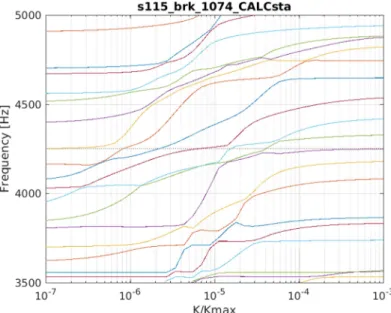
This paper presents preliminary results where a single stiffness factor 𝛼 identically applied to the 4 junctions. Computation is performed between 𝛼 = 10 and 𝛼 = 10 (no evolution outside) and Figure 7 shows the evolution of mode frequencies with the parameter. When the stiffness increases, modal frequencies rise up and several shape crossings pass through 4250Hz (the squeal occurrence and thus expansion frequency).
Figure 7 : Mode frequency evolution with the parameter evolution
Figure 8 presents the parametric stability diagram (or root locus) for the study. This highlights the strong sensitivity of modal damping, thus confirming the interest for the parameters pointed by the initial MDRE analysis on squeal stability.
To get the optimal parameter, the relative model error is shown on Figure 9.
Figure 9 : Relative error of model in function of the stiffness parameter for the first shape (left) and the second shape (right)𝛾 = 10
For the first shape, two minima are reached at K/Kmax=6e-6 (global minimum) and K/Kmax=3e-5 (local minimum). Expanded shapes corresponding to these parameters are shown in Figure 10. The first is global while the second is a local bending of the wear indicator / edge of lower pad.
Figure 10 : Expansion of the first shape for the parameters K/Kmax=6e-6 and K/Kmax=3e-5
The same behavior occurs with the second shape with two minima reached at K/Kmax=8e-7 (local minimum) and K/Kmax=5e-5 (global minimum), whose expanded shapes are shown in Figure 11. One again sees either a global mode or the same local lower pad mode.
Figure 11 : Expansion of the second shape for the parameters K/Kmax=8e-7 and K/Kmax=5e-5
The existence of minima pointing to local unmeasured motion is the indication that local modes of this part may exist. Adding more measurement points would either remove the local minimum of the objective function or confirm the influence of that local mode on the squeal event near 4250 Hz. Vibration of the wear indicated was actually considered in design studies. Future investigations will address the following issues: the optimum parameter differs for the two test shapes so a consistent value must be found combining an objective on both shapes; the 4 parameters should be considered independently. Decoupling normal and tangential
stiffness in the contact parameterization is also possible. The crossing shapes in the S curves (Figure 7), probably corresponding to localized deformations shown in Figure 10 and Figure 11, must be analyzed using modal observations [8]. Finally, it would be interesting to look at the evolution of test/analysis correlation with updating using the MAC matrix.
CONCLUSION
This paper summarized the theory behind Minimum Dynamic Residual Expansion MDRE and showed it to be applicable to an industrial brake squeal problem. The expansion gives access to an estimate of the limit cycle shapes on the full set of DOF including hidden parts and junctions and it further gives model error evaluations that can be used to localize problems in the model based on the squeal shapes only. The evaluation of model error was used to define pertinent junction parameters that were later considered in an updating loop that did not show the usual irregularities that plague MAC based objective criteria.
While the theory behind MDRE has been known for decades, the combination of model reduction techniques proposed here was crucial to allow parametric studies in a reasonable time. The need to work on criteria for interpretation was illustrated by the distinction between model error on free and enrichment shapes, which was key to allow the clear localization of errors on the springs between the anchor bracket and pads. For the updating part, the need to consider more independent parameters and to introduce multi-shape objective criteria was also pointed out.
Other topics for future work are the consideration of relations between parametrization and bias in the updated parameters, understanding expanded shape errors in the presence of incorrect models for a given test wireframe density, and obviously the introduction of strategies that could hint on the impact of squeal mitigation measures.
REFERENCES
1. Martin G, Balmes E, Chancelier T. Review of model updating processes used for brake components. In: Eurobrake. 2015.
2. Martin G, Balmes E, Vermot Des Roches G, Chancelier T. Updating and design sensitivity processes applied to drum brake squeal analysis. In: Eurobrake. 2016 3. Martin G, Balmes E, Vermot Des Roches G, Chancelier T. Squeal measurement using
operational deflection shape. Quality assessment and analysis improvement using FEM expansion. In: Eurobrake. 2017
4. Balmes E. Review and Evaluation of Shape Expansion Methods. IMAC. 2000;555–61. 5. Bobillot A, Balmes E. Solving minimum dynamic residual expansion and using results for
error localization. Proc IMAC XIX SEM Kissimee. 2001
6. Martin G, Balmes E, Vermot Des Roches G, Chancelier T. Squeal measurement with 3D Scanning Laser Doppler Vibrometer: handling of the time varying system behavior and analysis improvement using FEM expansion. In: ISMA. KUL; 2018.
7. Allemang RJ. The modal assurance criterion (MAC): twenty years of use and abuse. Int Modal Anal Conf. 2002;397–485.
8. Martin G. Méthodes de corrélation calcul/essai pour l’analyse du crissement. 2017. 9. Hammami C. Intégration de modèles de jonctions dissipatives dans la conception