Recherche de Jupiters chauds autour d'étoiles jeunes

(1)

THÈSE

En vue de l’obtention du

DOCTORAT DE L’UNIVERSITÉ DE TOULOUSE

Délivré par : l’Université Toulouse 3 Paul Sabatier (UT3 Paul Sabatier)

Présentée et soutenue le 06/12/2019 par : Louise Yu

Recherche de Jupiters chauds autour d’étoiles jeunes

JURY

RIEUTORD Michel Président du Jury

DELEUIL Magali Rapportrice

DOUGADOS Catherine Rapportrice

BARUTEAU Clément Examinateur

BOUVIER Jérôme Examinateur

COLLIER CAMERON Andrew Examinateur

MOUTOU Claire Co-Encadrante

École doctorale et spécialité :

SDU2E : Astrophysique, Sciences de l’Espace, Planétologie Unité de Recherche :

Institut de Recherche en Astrophysique en Planétologie (IRAP, UMR 5277) Directeur de Thèse :

Jean-François DONATI Rapporteurs :

(2)

(3)

Abstract

The past 25 years have seen the detection of about 400 hot Jupiters (hJs), giant exoplanets similar to Jupiter but orbiting their star a hundred times closer than Jupiter does the Sun. These puzzling planets are believed to have formed far from their star before migrating inwards, however the physical processes that drive this orbital transfer are still poorly constrained by observations. This question, essential to our understanding of planetary system formation, has profound implications for the architecture of these systems, and in particular for the probability of forming planets like the Earth in the habitable zone of stars.

In order to better constrain the early orbital evolution of planetary systems, we analyze data collected within the frame of the MaTYSSE programme to search for hJs around weak-line T Tauri stars (wTTSs), i.e. very young Sun-like stars that stopped accreting. The main goal of MaTYSSE is to characterize the high magnetic activity of wTTSs. This activity makes hJ detection difficult, indeed, we look for hJs with the velocimetry technique, but the strong presence of magnetic dark spots and bright plages on the surface of wTTSs adds a jitter in the radial velocities (RVs), of much greater amplitude than that expected of a hJ signature.

In this thesis, we model the magnetic activity of wTTSs TAP 26 and V410 Tau and filter the activity jitter out of their RVs. We also present the MaTYSSE results for star V830 Tau, for comparison. Using Zeeman-Doppler Imaging on spectropolarimetric data sets to reconstruct surface brightness distributions and magnetic topologies, we derive spot-and-plage coverages of 10 – 18 % and field strengths of 300 – 600 G. All three stars exhibit intrinsic variability not explained by differential rotation.

The activity jitter is modelled with two independent methods: deriving it from our ZDI maps, or applying Gaussian Process Regression to the raw RVs. Both methods concur on the detection of a hJ around V830 Tau and another around TAP 26. The ∼2 Myr V830 Tau b has a M sin i of 0.57 ± 0.10 MJup and orbits at 0.057 ± 0.001 au from its star (orbital period ∼4.93 d). Due

to the observing window, the orbital period of TAP 26 b cannot be uniquely determined; the case with highest likelihood is a hJ with M sin i = 1.66 ± 0.31 MJup on an orbit of semi-major

axis 0.0968 ± 0.0032 au (orbital period 10.79 ± 0.14 d). These detections suggest that type II disc migration is efficient at generating newborn hJs, and that hJs may be more frequent around young stars than around mature stars, or the MaTYSSE sample is biased towards hJ-hosting stars.

Our V410 Tau RVs exclude the presence of a Jupiter-mass companion below ∼0.1 au, which is suggestive that hJ formation may be inhibited by the early depletion of the circumstellar disc, which for V410 Tau may have been caused by the M dwarf stellar companion orbiting a few tens of au away.

(4)

Resumé

Les 25 dernières années ont vu la détection d’environ 400 Jupiters chauds (hJs), exoplanètes géantes semblables à Jupiter mais sur des orbites cent fois plus resserrées. Ces planètes étonnantes se seraient formées loin de leur étoile avant de migrer vers elle, cependant les processus physiques à l’origine de ce transfert orbital sont encore peu contraints par les observations. Cette question, essentielle à notre compréhension de la formation des systèmes planétaires, a de profondes répercus-sions sur l’architecture de ces systèmes, et en particulier sur la probabilité de former des planètes telles que la Terre dans la zone habitable des étoiles.

Afin de mieux contraindre l’évolution orbitale précoce des systèmes planétaires, nous analysons des données recueillies dans le cadre du programme MaTYSSE pour rechercher des hJs autour d’étoiles T Tauri à raies faibles (wTTSs), c’est-à-dire de très jeunes étoiles de type solaire qui n’ac-crètent plus. L’objectif principal de MaTYSSE est de caractériser l’importante activité magnétique des wTTSs. Cette activité rend la détection de hJs difficile, en effet, nous recherchons des hJs par la technique de vélocimétrie, mais la forte présence de taches sombres et de plages brillantes magné-tiques à la surface des wTTSs ajoute une perturbation dans les vitesses radiales (RVs), d’amplitude bien supérieure à celle attendue d’une signature de hJ.

Dans cette thèse, nous modélisons l’activité magnétique des wTTSs TAP 26 et V410 Tau et filtrons la perturbation des RVs due à l’activité. Nous présentons également les résultats MaTYSSE sur l’étoile V830 Tau pour comparaison. En utilisant l’imagerie Zeeman-Doppler sur des jeux de données spectropolarimétriques pour reconstruire les distributions surfaciques de brillance et les topologies magnétiques, nous obtenons des couvertures en taches et plages de 10 – 18 % et des champs de 300 – 600 G. Les trois étoiles présentent une variabilité intrinsèque non expliquée par la rotation différentielle.

La perturbation RV due à l’activité est modélisée à l’aide de deux méthodes indépendantes : nous la dérivons à partir de nos cartes ZDI, ou nous appliquons la régression par processus gaussiens aux RVs brutes. Les deux méthodes s’accordent sur la détection d’un hJ autour de V830 Tau et d’un autre autour de TAP 26. V830 Tau b, âgé de ∼2 Myr, a un M sin i de 0.57 ± 0.10 MJup et orbite à

0.057 ± 0.001 au de son étoile (période orbitale ∼4.93 d). La période orbitale de TAP 26 b ne peut être déterminée de façon unique à cause de la fenêtre d’observation ; le cas le plus probable est un hJ avec M sin i = 1.66 ± 0.31 MJup sur une orbite de demi-grand axe 0.0968 ± 0.0032 au (période

orbitale 10.79 ± 0.14 d). Ces détections suggèrent que la migration de type II dans le disque est efficace pour générer des hJs nouveau-nés, et que les hJs sont peut-être plus fréquents autour des étoiles jeunes qu’autour des étoiles matures, ou que l’échantillon MaTYSSE est biaisé vers les étoiles hôtes de hJs.

Nos RVs de V410 Tau excluent la présence d’un compagnon de masse Jovienne en-deçà de ∼0.1 au, ce qui suggère que la formation de hJs est peut-être inhibée par l’épuisement précoce du disque circumstellaire, qui pour V410 Tau aurait été causé par le compagnon stellaire, une naine M orbitant à quelques dizaines de au de l’étoile.

(5)

Remerciements

Tout d’abord, un énorme merci à Magali et Catherine pour avoir bien voulu lire et évaluer mon ma-nuscrit en un intervalle de temps restreint. Merci bien sûr à Jean-François, sans qui cette thèse n’au-rait pas eu lieu, pour ton accompagnement durant presque quatre ans, pour ta patience, le temps que tu as toujours pu me consacrer, et pour tout ce que tu m’as appris. Merci beaucoup à Claire et Clément pour des discussions toujours enrichissantes et pour votre bonne humeur constante. Enfin, merci à Michel, Andrew et Jérôme d’avoir bien voulu être examinateurs de ma soutenance et pour des discussions intéressantes pendant ma thèse.

Ces trois ans et demi ont été l’occasion de former de belles amitiés, qui ont agrémenté ce passage de vie particulier de précieux moments de bonheur. Un merci plein de tendresse donc aux Bras Cassés : Adrien, Mathilde, Edo, Pauline, Geoffroy, pour les jeux, les soirées, les rires. Et un grand merci à Babak, pour tous les fous rires, la musique, ton soutien, ton aide, ta bonne humeur et ta joie de partager inépuisables.

Je remercie l’équipe du PS2E pour leur accueil, pour les discussions, les Journal Clubs, les workshops : les sus-mentionnés Clément et Michel, mais aussi Pascal, Arturo, Laurène (merci pour l’école SunStars à Banyuls !), Sébastien. Merci également à tous ceux, au sein de l’IRAP, qui m’ont aidée à diverses occasions : Geneviève, Émilie, Carole, Patricia, Isabelle, Loïc.

A special thank you to those who welcomed me in St Andrews in October 2017 : Andrew and Moira, and the students Josh, Chris, Dom, Laith, Kirsten, Meng and Fran for the Friday meals and game nights. Finally, thanks to Paloma for your company and to Maries for hosting me.

Merci également à toute l’équipe d’UniverSCiel, pour d’inoubliables moments lors des festivals astrojeunes et autres sorties : Marina, Gab, Wilou, Turpin, Jason, Ppeille, Tata, Lulu, Neuha, Heussaff, Edo, Didi, Jeff, Babak, Ines, Damien, Sacha, Gabi, Simon, Mika, PM, Momo, Hadrien, Mehdi, Abe.

Je remercie tous les doctorants et post-doctorants qui sont passés à l’IRAP avant, en même temps et après moi, pour les conseils, les discussions, les parties de tarot et, pour certains, leur amitié : CHill, Colin F, Andres, Logithan, Elodie, Giovanni, Cyril, Damien, Ppeille, Wrappin, Fitouss, Kevin, Nicolas, Jessie, David, Najda, Annick, Armelle, Étienne, Damien, Gaylor, Paul, Abe, Anthony, Bonnie, Tianqi, Benjamin, Nu, Grégoire, Paul, Benjamin, Florian, Ludivine, Mélina, Léo, Mégane.

Merci aux amis d’horizons divers, pour certains loin de Toulouse, mais toujours là dans ma vie : Antoine, Audrey, Florian, Marine, Raphaël, Élise, Ao, Julien, Luana, Marion, Ambroise, Momo, Fred, Lina, HS, Jenn, Lilly, Claire et Lætitia.

Et enfin, le plus grand des mercis à ma famille, Maman, Papa, Raph, qui ont toujours été là pour moi, merci pour votre soutien et votre amour inconditionnels, j’ai beaucoup de chance de vous avoir.

(10)

(11)

Foreword

The search for exoplanets has yielded around 4000 confirmed detections in the past 30 years, in around 3000 planetary systems. Those extrasolar systems are of very diverse configurations, with many tightly-packed systems of terrestrial planets all on orbits smaller than the orbit of Mercury, some systems with one or several gas giants as massive as Jupiter or Saturn, a few systems orbiting two stars (Winn & Fabrycky, 2015)... A few candidate Solar system analogs, with a gas giant on a low-eccentricity orbit of several astronomical units around a Sun-like star, were detected as well (Barbato et al., 2018). Simultaneously to observational efforts of establishing exoplanetary population statistics, theories on the formation and evolution of planetary systems were developed to explain the current diversity of orbital configurations, and eventually assess how much of an exception the Solar system is (e.g. Mordasini, 2018).

In particular, the origins of hot Jupiters (hJs), i.e. giant planets on close-in orbits, estimated to occur around ∼1 % of Sun-like stars (Wright et al., 2012), are mysterious. In-situ formation in the protoplanetary disc, the primordial dust and gas planet-forming matrix around the forming star, has long been considered implausible, because the high keplerian velocities and the limited quantity of material close to the star make it difficult to build up sufficiently massive cores. Some recent studies have argued in favor of it (e.g. Batygin et al., 2016), but its feasibility is still debated (Dawson & Johnson, 2018). Two theories suggesting that giant planets form far from the star and then migrate inwards have been proposed. Such massive planets have a large gravitational influence impacting their whole planetary systems, constraining their migration would therefore be an essential first step to model the evolution of planetary systems. Shortly after the first confirmed detection of a planet around a Sun-like star (Mayor & Queloz, 1995), a circular hJ in fact, Lin et al. (1996) showed that a scenario where the giant planet migrated within its protoplanetary disc through interactions with the surrounding dust and gas, on a time scale shorter than the lifetime of the disc (∼1 Myr), could explain the observations. As more giant planets got detected, their distributions of orbital eccentricities and of obliquities, depending on the distance separating them to their host star, led to another scenario where gravitational interactions between planets and with their star caused instabilities, sending them on eccentric and inclined orbits. Those which were sent on orbits crossing the influence area of stellar tidal forces would then lose orbital energy and see their orbit become circular again, over time scales of 102 _{– 10}3_{Myr (Dawson & Johnson,}

2018). The study of hJs aged a few Myr, around stars whose protoplanetary discs have dissipated, can therefore be a key element to investigate which migration processes dominate.

However, Sun-like stars of a few Myr that have lost their discs, called weak-line T Tauri stars (wTTSs), have an important magnetic activity that causes large-amplitude modulations of their measured luminosity and radial velocity (RV; Grankin et al., 2008; Crockett et al., 2012). As a result, potential hints of a planetary presence, either a dip in the light curve betraying a transiting planet, or a wobble in the RV curve indicating the star’s reflex motion from the planet’s gravitational pull, are drowned in variations an order of magnitude larger than the expected planetary signature amplitudes. Astronomers have studied the variability and activity of wTTSs since the mid-20th century, but the research for hJs around them had to wait for the advent of spectropolarimetry,

(12)

combined with magnetic imaging techniques, and its application to wTTS targets. This thesis is part of one of the pioneering programmes in the search for young hJs: MaTYSSE (Donati et al., 2014).

More precisely, MaTYSSE, which stands for Magnetic Topologies of Young Stars and the Sur-vival of close-in massive Exoplanets, aims at characterizing the magnetic activity of wTTSs, com-paring it to the magnetic activity of Sun-like stars at earlier and later evolution stages, and searching for hJs around them. It is based upon the spectropolarimetric monitoring of 35 wTTSs, with ob-servations collected between 2013 and 2016 with the twin echelle spectropolarimeters ESPaDOnS (Donati, 2003), installed at the Canada-France-Hawaii Telescope (CFHT), Hawaii since 2004, and NARVAL, installed at the Télescope Bernard Lyot (TBL), France since 2006. From the spectra pro-vided by these instruments, both unpolarized and circularly polarized, we use the Zeeman-Doppler Imaging (ZDI) technique, first developed in the 90s (Semel, 1989) and having undergone successive updates until 2014 (Donati et al., 2014), to reconstruct the surface distribution of brightness and of magnetic field for our wTTSs. Because RVs are measured from the spectral lines in the unpolarized spectra, the activity RV jitter originates from distorsions of the spectral lines mainly due to surface brightness inhomogeneities; therefore our ZDI brightness maps are used to model the activity RV jitter and filter it out, in order to investigate the potential presence of hJ signatures in the filtered RV curves. ZDI has proven an efficient filtering technique for wTTSs prior to this thesis, with the first two MaTYSSE papers on stars LkCa 4 (Donati et al., 2014), V819 Tau and V830 Tau (Donati et al., 2015).

This thesis presents the investigation of the activity and RVs of two more MaTYSSE stars, ∼17 Myr, ∼1 M TAP 26 and ∼0.8 Myr, ∼1.4 M V410 Tau, as well as V830 Tau, on which more

recent data sets were collected. On top of using ZDI, another numerical technique is applied, called Gaussian Process Regression (GPR) and first proposed to the application of exoplanet hunting by velocimetry in Haywood et al. (2014). Applied directly to the raw RVs, GPR is a technique independent from ZDI, that does not rely on a physical model but assumes a given statistical behaviour of the RV curve, with the RV activity jitter being described as a correlated noise. The modelling process thus consists in finding the main parameters characterizing this statistical behaviour, providing at the same time information on the stellar activity.

The first chapter outlines the context of the whole study and presents the broad lines of what constitutes the current theories of star and planet formation and early evolution; in a second chapter, we detail the problem of modelling wTTS activity and describe the various complementary modelling techniques used for this work; chapter three then presents the results of applying our activity modelling techniques to TAP 26, V410 Tau and V830 Tau, and chapter four presents the investigation of the RV curves of these stars. Finally, we draw some conclusions that this thesis brought to the field of star and planet formation, and give some future perspectives.

(13)

Avant-propos

La recherche d’exoplanètes a donné lieu à environ 4000 détections confirmées au cours des 30 dernières années, dans environ 3000 systèmes planétaires. Ces systèmes extrasolaires sont de confi-gurations très diverses, avec de nombreux systèmes de planètes telluriques très resserrés, sur des orbites plus petites que celle de Mercure, certains systèmes avec une ou plusieurs géantes gazeuses aussi massives que Jupiter ou Saturne, quelques systèmes en orbite autour de deux étoiles (Winn & Fabrycky, 2015)... Quelques systèmes potentiellement analogues du système solaire, avec une géante gazeuse sur une orbite à faible excentricité de plusieurs unités astronomiques autour d’une étoile semblable au Soleil, ont également été détectés (Barbato et al., 2018). Parallèlement aux efforts d’observation visant à établir des statistiques sur les populations exoplanétaires, des théories sur la formation et l’évolution des systèmes planétaires ont été élaborées pour expliquer la diversité actuelle des configurations orbitales, et finalement évaluer dans quelle mesure le système solaire fait exception (voir par exemple Mordasini, 2018).

En particulier, les origines des Jupiters chauds (hJ), planètes géantes placées sur des orbites resserrées, dont la fréquence autour des étoiles semblables au Soleil est estimée à ∼1 % (Wright et al., 2012), sont mystérieuses. La formation in-situ dans le disque protoplanétaire, la matrice de poussière et de gaz autour de l’étoile et des planètes en formation, a longtemps été considérée comme improbable, car les vitesses képlériennes élevées et la quantité limitée de matière à proxi-mité de l’étoile rendent difficile la constitution de noyaux suffisamment massifs. Certaines études récentes ont plaidé en sa faveur (par exemple Batygin et al., 2016), mais sa faisabilité est encore débattue (Dawson & Johnson, 2018). Deux théories suggérant que les planètes géantes se forment loin de l’étoile et migrent ensuite vers l’intérieur ont été proposées. De telles planètes massives ont une grande influence gravitationnelle qui a un impact sur l’ensemble de leur système planétaire, comprendre leur migration serait donc une première étape essentielle pour modéliser l’évolution des systèmes planétaires. Peu après la première détection confirmée d’une planète autour d’une étoile semblable au Soleil (Mayor & Queloz, 1995), qui était d’ailleurs un hJ sur orbite circulaire, Lin et al. (1996) a montré qu’un scénario où la planète géante migrait à l’intérieur de son disque protoplanétaire par des interactions avec la poussière et le gaz environnant, sur une échelle de temps plus courte que la durée de vie du disque (∼1 Myr), pourrait expliquer les observations. Au fur et à mesure que des planètes géantes furent détectées, la distribution de leurs excentricités et de leurs obliquités orbitales, en fonction de la distance qui les sépare de leur étoile hôte, a conduit à un autre scénario où les interactions gravitationnelles entre les planètes et avec leur étoile pro-voquent des instabilités, les envoyant sur des orbites excentriques et inclinées. Celles qui étaient envoyées sur des orbites traversant la zone d’influence des forces de marée stellaires perdraient alors de l’énergie orbitale et verraient leur orbite redevenir circulaire, sur des échelles de temps de 102 _{– 10}3_{Myr (Dawson & Johnson, 2018). L’étude des hJs âgés de quelques Myr, autour d’étoiles}

dont les disques protoplanétaires se sont dissipés, peut donc être un élément clé pour étudier les processus de migration.

Cependant, les étoiles de quelques Myr, semblables au Soleil, qui ont perdu leurs disques, appe-lées étoiles T Tauri à raies faibles (wTTS), ont une activité magnétique importante qui provoque

(14)

des modulations de grande amplitude dans leurs courbes de luminosité et de vitesse radiale (RV ; Grankin et al., 2008; Crockett et al., 2012). Par conséquent, les indices potentiels d’une présence pla-nétaire, soit une baisse de la courbe de lumière trahissant une planète en transit, soit une oscillation de la courbe RV indiquant le mouvement réflexe de l’étoile causé par l’attraction gravitationnelle de la planète, sont noyés dans des variations d’un ordre de grandeur supérieur aux amplitudes at-tendues des signatures planétaires. Les astronomes ont étudié la variabilité et l’activité des wTTSs depuis le milieu du 20e siècle, mais la recherche des hJs autour d’elles a dû attendre l’avènement de la spectropolarimétrie, combinée aux techniques d’imagerie magnétique, et leur application aux wTTSs. Cette thèse fait partie d’un des programmes pionniers dans la recherche de jeunes hJs : MaTYSSE (Donati et al., 2014).

Plus précisément, MaTYSSE, qui signifie Magnetic Topologies of Young Stars and the Survival of close-in massive Exoplanets, vise à caractériser l’activité magnétique des wTTSs, à la comparer à celle des étoiles semblables au Soleil à des stades d’évolution antérieurs et postérieurs, et à rechercher des hJs autour de ces wTTSs. Le programme se base sur le suivi spectropolarimétrique de 35 wTTSs, avec des observations collectées entre 2013 et 2016 avec le spectropolarimètre à échelle ESPaDOnS (Donati, 2003), installé au Télescope Canada-France-Hawaï (CFHT), Hawaï depuis 2004, ainsi que son jumeau NARVAL, installé au Télescope Bernard Lyot (TBL), France depuis 2006. À partir des spectres, non polarisés et polarisés circulairement, fournis par ces instruments, nous utilisons la technique d’imagerie Zeeman-Doppler (ZDI), développée pour la première fois dans les années 90 (Semel, 1989) et ayant subi des mises à jour successives jusqu’en 2014 (Donati et al., 2014), pour reconstruire la distribution surfacique de brillance et de champ magnétique de nos wTTSs. Les RVs étant mesurées à partir des raies spectrales des spectres non polarisés, la perturbation d’activité des RVs provient des distorsions des raies spectrales essentiellement dues aux inhomogénéités de brillance surfacique ; par conséquent, nos cartes de brillance ZDI sont utilisées pour modéliser la perturbation d’activité des RVs et la soustraire de notre signal, afin d’explorer la présence potentielle de signatures de hJs dans les courbes de RVs filtrées. ZDI a prouvé son efficacité en tant que technique de filtrage pour les wTTSs avant cette thèse, avec les deux premiers articles MaTYSSE sur les étoiles LkCa 4 (Donati et al., 2014), V819 Tau et V830 Tau (Donati et al., 2015).

Cette thèse présente l’étude de l’activité et des RVs de deux autres étoiles MaTYSSE : TAP 26, âgée de ∼17 Myr et de masse ∼1 M, et V410 Tau, âgée de ∼0.8 Myr et de masse ∼1.4 M. Des

résultats sur des jeux de données plus récents de la wTTS V830 Tau sont également présentés. En plus de l’utilisation de ZDI, une autre technique numérique est utilisée, appelée Régression par Processus Gaussiens (GPR) et appliquée pour la première fois à la recherche d’exoplanètes par vélocimétrie dans Haywood et al. (2014). Appliquée directement aux RVs brutes, GPR est une technique indépendante de ZDI, qui ne repose pas sur un modèle physique mais qui suppose un comportement statistique donné de la courbe des RVs, la perturbation d’activité des RVs étant décrite comme un bruit corrélé. Le processus de modélisation consiste donc à trouver les princi-paux paramètres caractérisant ce comportement statistique, en fournissant en même temps des informations sur l’activité stellaire.

Le premier chapitre décrit le contexte d’ensemble de l’étude et brosse un portrait grossier des théories actuelles sur la formation et de l’évolution précoce des étoiles et des planètes ; dans un deuxième chapitre, nous détaillons le problème de la modélisation de l’activité des wTTSs et décrivons les différentes techniques de modélisation complémentaires utilisées pour ce travail ; le chapitre trois présente ensuite les résultats de l’application de nos techniques de modélisation de l’activité à TAP 26, V410 Tau et V830 Tau, et le chapitre quatre présente l’étude des courbes RV de ces étoiles. Enfin, nous tirons quelques conclusions que cette thèse a apportées au domaine de la formation des étoiles et des planètes, et donnons quelques perspectives d’avenir.

(15)

1 |

Introduction: the formation of stars

and their planets

Contents

1.1 A few notions on the diversity of stars and exoplanets . . . . 8

1.1.1 Stages of stellar evolution . . . 8

1.1.2 The diversity of exoplanetary systems . . . 9

1.2 The formation of stars . . . . 10

1.2.1 From molecular clouds to protostars . . . 11

1.2.2 Classical T Tauri stars . . . 13

1.2.3 Weak-line T Tauri stars . . . 14

1.3 Protoplanetary discs . . . . 15

1.3.1 Structure . . . 15

1.3.2 From dust particles to planets . . . 16

1.4 The mystery of hot Jupiters . . . . 17

1.4.1 Two theories of giant planet migration . . . 17

1.4.2 In-situ formation? . . . 18

1.4.3 Further orbital migration . . . 18

(16)

1.1 A few notions on the diversity of stars and exoplanets

1.1.1 Stages of stellar evolution

Stars form in clouds of dust and gas, accreting plasma until they reach a stable mass. This mass, which varies between ∼0.1 – 100 solar masses (M), is the predominant factor that determines a

star’s evolution. In particular, one can follow the path of a star along its life on a temperature-luminosity plot, or Hertzsprung-Russell (HR) diagram (see figure 1.1). The main sequence (MS) is a region of the HR diagram where stars spend most of their life: it corresponds to the stage during which they burn hydrogen through nuclear fusion in their cores. In general, the more massive a star is, the hotter and brighter it is on the MS, and the faster it evolves through the various evolutionary stages described in the following paragraphs.

Figure 1.1 – Some famous stars on the Hertzsprung-Russell diagram. Masses and lifetimes are noted along the main sequence. Source: https://www.eso.org/public/images/eso0728c/ through https:// commons.wikimedia.org/wiki/File:Hertzsprung-Russel_StarData.png.

◦ The most massive stars (M? & 8 M) reach the MS at ages 0.02 – 0.2 Myr. They initiate

hydrogen nuclear fusion in their cores before they have finished accreting their mass, then stay on the MS until ages 3 – 100 Myr (Maeder, 2009, chapter 18). When they have exhausted the

(17)

hydrogen reserves in their cores, they leave the MS and enter an inflated state as supergiants for 0.5 – 5 Myr, during which they fuse progressively heavier elements in their cores, until developping an iron core, at which point they explode into supernovae and their cores collapse into neutron stars or black holes (Maeder, 2009).

◦ Stars of masses ∼0.5 – 8 M reach the MS at ages 0.2 – 100 Myr and stay on the MS until

ages 0.1 – 10 Gyr. When they exhaust their core hydrogen fuel, they inflate into red giants, fusing helium at their core for 0.5 – 103_{Myr. After running out of nuclear fuel (they are not}

massive enough to initiate full-scale carbon fusion), these stars contract, expelling their outer layers into planetary nebulae through superwinds. Their cores then cool down to become white dwarfs.

◦ Low-mass stars (M_?_{. 0.5 M}) have a lifetime longer than the age of the Universe, and what

happens to them after leaving the MS is yet unobserved.

At the beginning of their life, stars of masses . 8 M go through a protostar phase, during

which they accrete most of their mass, and a pre-main sequence (PMS) phase, during which they contract towards the MS. For stars of masses ∼0.5 – 2 M, the PMS track on the HR diagram

is composed of a phase of luminosity decrease at roughly constant temperature (Hayashi track) and a phase of temperature increase at roughly constant luminosity (Henyey track). These stars follow the Hayashi track for 2 – 20 Myr, during which their interiors are fully convective, and they bifurcate on the Henyey track when a radiative core starts developing. Stars of lower masses stay fully convective, so they follow the Hayashi track up to the MS, and stars of higher masses spend their PMS phase following the Henyey track (e.g. Bodenheimer, 2011, chapter 8).

Protostars and some PMS stars are embedded in circumstellar dust and gas, from which they grow; a protostar/PMS star and its circumstellar environment is referred to as a young stellar object (YSO). YSOs are extensively studied to constrain the theories of stellar formation, for example to explain observed distributions of masses (see studies about the Initial Mass Function, e.g. Offner et al., 2014) and of multiplicity (e.g. solar-type MS stars have on average ∼ 0.6 stellar companion gravitationally bound to them, Duchêne & Kraus, 2013) among MS stars. Moreover, planets can form from the circumstellar matter around PMS stars; therefore, investigating YSOs is also important to understand the initial conditions of the evolution of planetary systems.

1.1.2 The diversity of exoplanetary systems

The search for exoplanets, i.e. planets orbiting around stars other than the Sun, has yielded about 4000 confirmed detections as of 2019 October. Traditionally, a substellar object orbiting a star was classified as a planet if its mass was below 13 Jovian masses (MJup), and as a brown dwarf otherwise,

that criterion roughly corresponding to the start of the thermonuclear fusion of deuterium in the core (Boss et al., 2007). However the distinction between giant planets and brown dwarfs is still debated as of today (e.g. Schneider, 2018).

Various observation/detection techniques exist, complementing each other (see e.g. Perryman, 2018, for a comprehensive review). Velocimetry (see section 2.4.1) yields orbital periods, lower boundaries on planet masses and orbital eccentricities. Photometry enables to detect transiting planets (planets passing between their host star and the observer), giving access to their radii and orbital periods, potentially to their eccentricities and planetary albedos, as well as an estimate of their masses in multiplanetary systems (from transit time variations, see e.g. Holman et al., 2010). Spectroscopy of transiting planets’ host stars unveils their sky-projected obliquities, i.e. the incli-nations between planets’ orbital axes and their hosts’ rotation axes (Rossiter-McLaughlin effect, see e.g. Fabrycky & Winn, 2009), as well as, potentially, some atmospheric characteristics (Mad-husudhan, 2019). Other observation/detection techniques include direct imaging and gravitational lensing, which enable the detection of planets located far from their host stars.

(18)

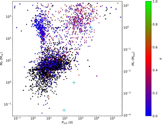
Figure 1.2 shows a mass/period diagram of confirmed exoplanets. Three populations stand out: the super-Earths (planets of masses ∼1 – 10 Earth masses), the hot giants (massive planets on close-in orbits) and the warm giants (massive planets on intermediate orbits). Many observed systems have architectures that are strikingly different from that of the Solar system (Winn & Fabrycky, 2015): for example, accounting for observational biases, it is estimated that ∼30 – 50 % of Sun-like stars have a super-Earth on an orbit closer-in than Mercury’s, while ∼10 % host a giant planet, usually on either a close-in orbit or a larger one but significantly eccentric (Raymond et al., 2018). The occurrence rate of hot Jupiters, the most massive of hot giants, was estimated at ∼1 % around Sun-like stars (Wright et al., 2012).

10 4 10 3 10 2 10 1 100 101 MP (MJup ) 10 1 ₁₀0 ₁₀1 ₁₀2 ₁₀3 ₁₀4 ₁₀5 Porb(d) 10 1 100 101 102 103 MP (M ) 0.0 0.2 0.4 0.6 0.8 1.0 e

Figure 1.2 – Exoplanets mass-period plot, with the color scale representing the orbit eccentricity, when known. Cyan crosses represent, from left to right, Mercury, the Earth and Jupiter. The data was downloaded from http://exoplanet.eu (Schneider et al., 2011) on 2019 October 28, totalling 3725 exoplanets. The masses of 851 among them were known (diamond symbols), those of 768 others were assimilated to their known lower boundaries (triangular symbols), and those of the 2106 remaining planets were derived from their radii (circular dots), following the method described in Han et al. (2014).

Because planets form together with their star, investigating the processes at play early in the life of stars and of their stellar/planetary systems is a primordial first step to understand the evolution of planetary systems, to explain their observed statistics (e.g. Mordasini, 2018), to assess how much of an exception the Solar system is and to estimate the likelihood of finding Solar-System analogs in the galaxy (e.g. Agnew et al., 2018; Barbato et al., 2018). In the next section, we present the broad lines of the current paradigm of stellar formation.

1.2 The formation of stars

YSOs are often seen in groups, whether in gravitationally bound clusters or in associations, within which age and proper motion are roughly homogeneous. These groups bathe in giant clouds of

(19)

gas and dust and are called star-forming regions (SFRs). Famous examples of SFRs are: the Taurus-Auriga molecular cloud, located ∼140 pc away from Earth (Galli et al., 2018), the Orion cloud (∼390 pc, Kounkel et al., 2017), the Scorpius-Centaurus association (∼140 pc, de Zeeuw et al., 1999), the ρ Ophiuchi nebula (∼140 pc, Ortiz-León et al., 2017)... It is noted that many SFRs are located in a particular region of the galaxy, the Gould Belt: an elliptic ring of semi-major and semi-minor axes ∼350 pc and ∼230 pc respectively, whose center lies ∼100 pc away from the Sun in the direction opposite to the galactic center (e.g. Perrot & Grenier, 2003), but the physical origin of the Gould Belt is debated (see e.g. Bobylev, 2014; Bouy & Alves, 2015).

The current understanding is that stars are born from the gravitational collapse of dense cores within these clouds, first appearing at the center of the collapsing core and then growing by matter accretion. Best seen in infrared wavelengths, YSOs are categorized into four classes (0, I, II and III) depending on their spectral energy distribution (SED), each class corresponding to an evolutionary stage as illustrated in figure 1.3 (Adams et al., 1987; André, 2015).

1.2.1 From molecular clouds to protostars

Dark regions have been observed in the sky, with low densities of apparent stars. We now know that they are clouds of gas and dust that dim the light coming from background stars. These clouds are composed in large majority of molecular Hydrogen (H2), with small amounts of interstellar

dust and traces of other molecular gases: CO, NH3, HCN, etc (see e.g. Wilson et al., 1970). Lada

(1992) among others showed that molecular clouds are major sites of stellar formation. André et al. (2014) observed that molecular clouds have a filamentary structure, with filaments always roughly 0.1 pc thick and preferentially in the direction of the cloud elongation. At the crossing of filaments, or at various places along these filaments, we can observe denser clumps, called pre-stellar cores, which are defined as the immediate vicinity of local minima of the gravitational potential within the cloud.

Magnetism and turbulence are thought to be the main factors that drive star formation (Bo-denheimer, 2011; Crutcher, 2012). In magnetically-controlled star formation scenarios, magnetic fields maintain the core against gravitational collapse but see their influence decrease as the core contracts and acquires mass (ambipolar diffusion), until the core reaches a critical mass and col-lapses. In turbulence-controlled star formation scenarios, supersonic turbulence within the cloud leads to complicated shock patterns that randomly generate highly-compressed regions that can collapse. Both magnetic fields and turbulence generally coexist at comparable levels in molecular clouds, so formation models including them together are favored (see Crutcher, 2012, for a review). Moreover, star formation can be triggered by factors external to the cloud, like supernovae shocks or cloud-cloud collisions, which create high-density regions that can collapse. YSOs clusters or associations are assumedly a result of either simultaneous collapse, where an external factor (such as galactic density waves) increases the density in the cloud on a global scale, or contagious star formation, where core collapses generate shockwaves that locally increase the density, resulting in more neighboring collapses (Maeder, 2009, Part V); turbulence can also lead to the simultaneous formation of several cores within a molecular cloud (Bodenheimer, 2011, Chapter 2).

Simulations of simplified cases (plasma ball with solid rotation and uniform magnetic field, e.g. Machida & Matsumoto, 2011; Machida & Basu, 2019) show that the birth of a protostar happens after two successive collapses (Masunaga & Inutsuka, 2000):

First collapse - When the density at the center of the pre-stellar core reaches ∼1010cm−3, the pressure at the center becomes high enough to create a shock, which defines the contour of what is called the first core. The first core accretes mass from the rest of the pre-stellar core, supported by thermal pressure and rotation against self-gravity (e.g. Wurster et al., 2018). The higher the

(20)

Figure 1.3 – Empirical sequence for the formation and circumstellar evolution of a single star from a prestellar cloud core to a class-III YSO, based on the shape of the SED (left), the bolometric temperature, and the mass of circumstellar (envelope + disc) material (right). The lifetime of a cTTS can in fact be as long as 10 Myr, making class-II and class-III phases hardly distinguishable in terms of age sample-wise. Source: André (2002).

initial angular momentum, the longer the first core lives before the second collapse, as centrifugal forces play against self-gravity to slow down the increase of density at its center. If given enough time, the first core takes a flattened shape before the second collapse, and the initial magnetic field

(21)

inside the first core gets dissipated by Ohmic and ambipolar diffusion, leading to a suppression of the magnetic braking (the magnetic field is no longer well-coupled to the neutral gas). Under some conditions, e.g. on the angle between the magnetic field and the angular momentum axis, the disc can become a Keplerian disc early on (see Hennebelle & Ciardi, 2009; Maury et al., 2019, for precise studies). During the accretion of the outer envelope by the first core, low-velocity outflows are driven from the outer boundary of the first core by magnetic forces, because magnetic field lines are twisted horizontally by the rotation (toroidal magnetic field). A very high angular momentum can lead to a fragmentation of the first core (Goodwin et al., 2007; Boss, 2009), which is one of the potential processes for generating multiple star systems (others being disc fragmentation post-protostar formation or gravitational capture; this question still constitutes an active field of research; see e.g. Goodwin et al., 2007; Maury et al., 2010).

Second collapse - When the temperature at the center of the first core reaches & 2000 K, the dissociation of H2 at the center changes the thermodynamics and triggers the second

col-lapse. This second collapse can be as fast as a few years, until the density at the center reaches ∼1018 _{– 10}20_cm−3_{, at which point we consider that the protostar is born. The rest of the first core}

surrounds the newborn class-0 protostar. If the angular momentum of the first core is very low, the first core remnant quickly falls onto the protostar. Otherwise, a Keplerian circumstellar disc appears (Machida & Matsumoto, 2011). Far from the star, in the outer envelope, the magnetic field is well coupled with the neutral gas, then in the area 1011_cm−3

. n . 1015cm−3, the dust absorbs the ions and the magnetic field is efficiently dissipated by Ohmic dissipation and ambipolar diffusion, letting the disc adopt a quasi-Keplerian rotation profile, then close to the star again, the degree of ionization increases and the magnetic field becomes coupled with the neutral gas again (Machida & Basu, 2019).

Main accretion phase - The main accretion phase starts, where the disc accretes mass from the primordial envelope which has not collapsed into the first core, while the protostar accretes mass from the surrounding disc. On top of the low-velocity outflows driven by the disc, high-velocity collimated jets appear near the protostar, fueled by disc material approaching the star at Keplerian velocities and being redirected outwards by toroidal magnetic fields. The accretion and jets are episodic, triggered by gravitational instabilities where clumps of material fall from the disc to the protostar, where a portion is evacuated as jets. The disc and the outer envelope are coupled by magnetic forces and exchange angular momentum, leading to a braking of the disc that prevents it from growing in size. The class-0 stage is characterized by a high mass ratio between the circumstellar environment and the protostar (Menv  M?) and lasts for a few 104yr (e.g. Andre et al., 2000; Masunaga & Inutsuka, 2000). During that phase, the protostar grows at an accretion rate of 10−6 _{– 10}−5_M

/yr (André, 2015). From an observational point of view, its SED is almost

the same as that of a prestellar core, but the presence of the protostar is betrayed by signatures of powerful highly-collimated jets (Bontemps et al., 1996; Bachiller, 1996). Eventually, the outer envelope depletes, allowing the disc to grow. A YSO enters class-I when the protostar becomes more massive than its circumstellar environment. Jets and outflows then broaden and weaken, and the accretion rate decreases to 10−7 _{– 10}−6_M

/yr (André, 2015). The envelope is still present but

the protostar signature appears in the SED at infrared wavelengths. The class I stage lasts for a few 105_{yr (Evans et al., 2009).}

1.2.2 Classical T Tauri stars

Eventually, the protostar has accumulated the majority of its mass and becomes a PMS star. It is at first a class-II source; a distinction is made between class-II YSOs of less than 2 M, called

(22)

classical T Tauri stars (cTTSs), and those of more than 2 M, called Herbig Ae/Be stars (we

do not discuss the latters). Having emerged from their now depleted envelope, cTTSs become visible at near-infrared and optical wavelengths, surrounded by an optically thick disc that causes an infrared excess in the SED (see figure 1.3). Material is channeled onto the star at a rate of 10−9 _{– 10}−7_M

/yr (André, 2015).

CTTSs were observed to have strong magnetic fields (several kG), amplified from the remnants of the primordial field by the dynamo of the star (Johns-Krull et al., 1999; Johns-Krull, 2007). These fields open a cavity around the star in the region where magnetic forces dominate over rotation, called the magnetospheric gap. At the edge of this gap, a magnetic coupling exists between the surface of the protostar and the disc (Collier Cameron & Li, 1994; Bessolaz et al., 2008), and accretion happens by funneling disc material along the magnetic field lines. This magnetic coupling induces a rotational braking of the star (Bouvier, 2007; Bouvier et al., 2014), especially in the propeller regime early on, when high-velocity jets are driven from the protostar (e.g. Romanova et al., 2004; Zanni & Ferreira, 2013).

Even though cTTSs are still contracting under their own gravity and gain angular momentum from the accretion, their rotation rates are observed to be much lower than expected (Rebull et al., 2004). Bouvier et al. (2014) provides a review of the sources of angular momentum gain/loss for cTTSs (star-disc interactions, stellar winds...), revising the widely used paradigm of disc-locking proposed by Ghosh & Lamb (1979), where the star would co-rotate with the inner edge of its disc because of magnetic locking between the stellar surface and the disc plasma. Though models have to be refined, it is still apparent that both the disc and the magnetic field play a major role in braking the star rotation. As the star evolves, its structure becomes more complex and so does its magnetic field, meaning the dipole weakens and the field strength quickly decreases with distance to the star. Thus the disc-braking is less and less efficient, eventually leading to a liberation of the star, which starts to spin up.

During this phase, dust grains can agglomerate within the disc, which can eventually lead to the formation of planetesimals and planets (see section 1.3.2).

1.2.3 Weak-line T Tauri stars

As the inner disc depletes due to its material being either accreted or ejected, accretion gets progressively weaker, then intermittent (cTTSs then become transitional T Tauri stars), before the inner disc is finally exhausted, and the star becomes a weak-line T Tauri star (wTTS, class-III YSO, see e.g. White et al., 2007). The age at which this transition occurs varies widely from star to star, being generally between 1 – 10 Myr (e.g. Richert et al., 2018), which implies that the population of . 10 Myr T Tauri stars is composed of both cTTSs and wTTSs, undistinguishable by age alone. The liberation from disc-locking can be triggered either by the dipole weakening as mentioned above, or by the dissipation of the disc. Free from disc-braking and still contracting, wTTSs spin up until age ∼10 – 100 Myr (depending on the mass). On the Hayashi track, the star shrinks at roughly constant temperature (4000 – 4500 K), then, around 1 – 3 Myr, it starts developing a radiative core and bifurcates on the Henyey track: the star keeps contracting, but at roughly constant luminosity and with a temperature rising with time, until reaching 4500 – 6500 K. For a 0.8 M star, the

contraction phase lasts for ∼25 Myr and for a 1.35 M star, it lasts for ∼10 Myr; stars shrink by a

radius factor of ∼20 – 60 (Amard et al., 2019).

After the contraction slows down, WTTSs spin down because of stellar winds until they reach the main sequence (see e.g. figure 1.4 for 1 M stars; for a more complete study, see Gallet &

Bouvier, 2015). The rotation periods of wTTSs reach down to ∼0.5 – 5 d when they spin the fastest (figure 1.4); their fast rotation induce a strong magnetic activity (see section 2.1.2).

(23)

OD Envelope Core

(a) 1 M

_⊙ OD Envelope Core

(b) 0.8 M

_⊙ OD Envelope Core

(c) 0.5 M

_⊙

Figure 1.4 – Figure extracted from Gallet & Bouvier (2015, figure 5). Angular velocity of the convective envelope (solid lines) and of the radiative core (dashed lines) shown as a function of time between 1 Myr and 10 Gyr for slow (red), median (green), and fast (blue) rotator models in a mass bin centered on 1 M. The left vertical axis is labelled with angular velocity normalised to the Sun’s, while the right vertical axis is labelled with rotational periods (days). The black crosses represent the observed angular velocities of stars in a selection of star-forming clusters of various ages. The red, green and blue tilted squares and associated error bars represent the 25th, 50th and 90th percentiles of the observed rotational distributions at each sampled age. The black rectangle labelled OD (lower right corner) shows the angular velocity dispersion of old disc field stars. The open circle is the angular velocity of the present Sun shown for reference, and the dashed black line illustrates Skumanich’s relationship (Skumanich, 1972), Ω ∝ t−1/2_.

1.3 Protoplanetary discs

We now focus on planetary formation within discs, called protoplanetary discs in this context. The content of this section is largely inspired from the review Armitage (2018).

1.3.1 Structure

We consider the disc around a cTTS (see figure 1.5). Discs around cTTSs have been observed to extend up to ∼100 astronomical units (au; e.g. TW Hya, Nomura et al., 2016). Their masses are estimated to be ∼10−3 _{– 10}−2 _{times the mass of the star (M}

?; see Andrews et al., 2013; Williams & Best, 2014). The surface density (volumic density integrated over the thickness of the disc) is expected to follow a law Σ ∝ r−1_{. Moreover, axisymmetric rings and non-axisymmetric structures}

in discs have been observed (e.g. ALMA Partnership et al., 2015; Dong et al., 2018), the origins of which are uncertain but are hypothesized to be tied to planetary formation (Baruteau et al., 2019). The disc is heated through various sources. Irradiation from the star leads to a global temper-ature profile T ∝ r−1/2_{(Kenyon & Hartmann, 1987). Close to the star, accretion heating increases}

the temperature in the mid-plane, leading to a vertical gradient of temperature (Armitage, 2018). Further away from the star, the thickness of the disc divides it into several regions: an isothermal inner region centered around the mid-plane, where Tdust= Tgas, then a warm layer of dust directly

(24)

Figure 1.5 –Cartoon of a protoplanetary disc viewed from the side (source: Armitage, 2018). The left part shows the thermal structure of the disc while the right part shows the magnetohydrodynamic regimes in various regions of the disc.

lines", which are the limits between areas where given chemicals are under solid or gaseous form. For example, the water snow line is located where T ' 150 K. Since the accretion heating wanes with time and the radius and temperature of the protostar evolve, the locations of the ice lines also evolve with time.

An important factor in the structure of the disc is the magnetic field. Close to the star (T > 3000 K), the disc is thermally ionized and the magnetic field is thus efficiently coupled with the gas. Further away, sources of non-thermal ionization (X-rays, UV photons or cosmic rays) are weak enough to let non-ideal MHD effects take place: the Ohmic diffusion and Hall effect decrease the influence of the magnetic field on the charged and neutral species, and beyond ∼ 30 au, the low density opens the way to ambipolar diffusion, where neutral species drift independently of the magnetic field, because the rate of collision with magnetically-tied electrons and ions is low. Magnetic fields also generate winds that participate to depleting the disc.

The phenomenon of photoevaporation, where gas heated by X-rays or UV photons escapes the disc, taking away matter and angular momentum, is most efficient at 2 – 3 au and can create a dip of density withing the disc, potentially even a gap, and eventually blow the disc away on long time scales.

1.3.2 From dust particles to planets

Not all mechanisms of planet formation within protoplanetary discs are understood as of today, especially as direct observation of disc-embedded planet formation is difficult. The paradigm of planetary formation is that of a bottom-up growth: dust grains (length scale: micrometer) aggregate into pebbles (cm), which themselves aggregate into planetesimals (km), some of which eventually grow into planets (Baruteau et al., 2016).

At first, when the dust grains are very small, aerodynamic forces dominate over gravitational forces, and dust grains grow from µm sized to mm sized thanks to 2-body collisions. Interactions

(25)

between the dust grains and their surrounding gas plays a role in the collision velocities and subsequent trajectory of the dust grains. These collisions, at first, can happen anywhere in the disc but as the solid grows, it is submitted to gas drag and tends to join the mid-plane and to drift radially towards the star. Bouncing and fragmentation are barriers to the growth of solids, and the critical relative velocities at which they happen depend on the solid composition (for example water ice is more resistant to fragmentation than silicates, Armitage, 2018). Eventually, these processes reach an equilibrium and the dust solids, now pebbles, can generally reach sizes of mm-cm, with pebble traps at the snow line and at the inner edge of the disc.

How pebbles grow into planetesimals is not well-constrained by observations, especially as meter-sized solids typically fall into the star in ∼100 yr from an original distance of 1 au, implying that planetesimal formation has to happen faster than solid infall into the star. Ideas proposed by the theory include porous growth, where pebbles stick to each other with little compression, giving birth to porous aggregates with increased cross sections, or streaming instability (Youdin & Good-man, 2005) where the disc gets fragmented and clumps of dust get trapped together, ending up aggregating.

As the planetesimals grow, gravitational forces become dominant and runaway growth starts. The heavier a planetesimal becomes, the faster its cross section grows thanks to its gravitational potential, and the more chances it has to collide with its neighbors. This phase leads to a size distribution of solids where a small number of very large planetesimals stand out. Pebble accretion can occur during this phase, where planetesimals absorb radially-drifting pebbles that arrive on their orbit.

Eventually, the biggest planetesimals, or oligarchs (103_{km), grow so massive that their}

inter-action with their neighbours scatters them, thus slowing down their growth. During this oligarchic growth phase, the oligarchs dominate the gravitational choreography: each of them settles into its own area of gravitational domination, and eventually "eats" the smaller planetesimals in this feeding zone, to grow into a planet embryo. Oligarchs can interact with each other, impacting their respective orbits and the general architecture of the system.

Finally, giant planets are formed from solid cores that have reached at least 10 – 15 Earth masses (M⊕), massive enough to trigger runaway accretion of a gaseous atmosphere from the surrounding

gas (Pollack et al., 1996). The time scale for forming such massive cores can be shorter than the lifetime of the disc, thanks to the enhancement of surface density beyond the snow line (e.g. Kennedy & Kenyon, 2008), and type I migration trapping solids near the snow line (see section 1.4.1).

1.4 The mystery of hot Jupiters

In 1995, the first confirmed detection of an exoplanet around a Sun-like star is published: 51 Peg b is a > 0.5 MJup planet orbiting at 0.05 au from its host (Mayor & Queloz, 1995). With only the

Solar System to compare at that time, finding a giant planet this close to the star was surpris-ing. Furthermore, such close-in orbits are not expected to provide favorable conditions for giant planet formation, since the high Keplerian velocities favor fragmentation during large planetesimal encounters, and the accretion of a massive gaseous envelope is difficult in the limited area around the orbit.

1.4.1 Two theories of giant planet migration

Disc migration - To explain the orbit of 51 Peg b, Lin et al. (1996) showed that giant planets can migrate within their protoplanetary disc from original distances of a few au to the inner edge of the disc, within the lifetime of the disc. In general, interactions between a forming planet and the

(26)

surrounding material in the protoplanetary disc impact the orbit of the planet, causing an orbital migration. The nature of the migration, caused by a wake torque and a corotation torque (Baruteau et al., 2016), depends on the mass of the planet and on properties of the disc. Planets below ∼10 M⊕ undergo type I migration, which generally drives them inwards (towards the star), except

around the silicate evaporation line and the water ice line. Outward migration around those lines and inward migration elsewhere create "planet traps" behind the silicate evaporation and water ice lines. Massive planets that open deep gaps in the disc around their orbits (masses typically & MJup)

undergo type II migration, which also drives them inwards on time scales & 104 _{– 10}5_{yr. Planets}

massive enough to open partial gaps in low- to moderate-density discs follow a migration regime intermediate between type I and type II, but in massive discs, they undergo type III migration which drives them outwards (Baruteau et al., 2016). Type II migration would enable to form hJs, generally keeping their orbit quasi-circular and coplanar. The planet still grows by accreting gas as it migrates, and the migration is slowed down when the planet mass becomes larger than the mass outside the planet gap. The migration stops when the planet reaches the inner edge of the disc. Eccentricity excitation and tidal circularization - Since 1995, ∼400 hot Jupiters have been detected (estimated masses between 0.5 – 13 MJup and orbital periods lower than 10 day, see figure

1.2 and its caption). Figure 1.6 shows the distribution of orbital eccentricities and sky-projected obliquities of giant planets. The eccentricities of hJs are generally low, whereas they are more dispersed for warm Jupiters. Few obliquities were measured for warm Jupiters, but we observe a large dispersion for hJs. A large eccentricity and/or a large obliquity are interpreted to result from gravitational interactions between oligarchs and/or fully-formed planets, which induce orbital instabilities (e.g. planet-planet scattering, Kozai-Lidov cycles, Dawson & Johnson 2018), changing their orbital angular momentums, eccentricities, semi-major axes and even potentially the planes of their orbits. For a cold giant planet to become a hJ, it would need to be placed on a highly eccentric orbit, with a periastron in the close-in region and an apoastron in the region where the planet originally was. The low eccentricities of hJs are believed to be the result of tidal circularization by the star: tidal forces work on the planet every time it goes through its periastron (close enough to be within reach of the stellar tidal influence), and the orbit circularizes within a few 102_{Myr. In}

the latter case, the obliquity does not get dampened as fast as the eccentricity (Dawson & Johnson, 2018).

1.4.2 In-situ formation?

Recent studies have argued in favor of in-situ formation of hot Jupiters, motivated by the difference of mass distribution between hot and cold Jupiters, and the detection of many 10 – 15 M⊕

exo-planets on very close-in orbits (Batygin et al., 2016). Batygin et al. (2016) ran simulations showing runaway accretion of a gaseous atmosphere onto 15 M⊕ cores at 0.05 au, however, simulations by

Coleman et al. (2017) taking different hypotheses showed no runaway atmosphere accretion on orbits below 0.1 au. The in-situ formation theory is still quite new and its feasibility not yet well established.

1.4.3 Further orbital migration

In the close vicinity of the host star, tidal and magnetic interactions between the star and the planet are strong enough to impact the orbit of the planet; in particular, these interactions transfer angular momentum between the star and the planet, by tending to synchronize the rotation of the star with the revolution of the planet. Thus, once a Jupiter-size planet reaches this region, depending on the geometry of the system, the hot Jupiter can either migrate slightly outwards or fall into the star (Bolmont & Mathis, 2016).

(27)

10

1

₁₀

0

₁₀

1

₁₀

2

₁₀

3

₁₀

4

₁₀

5

P

orb

(d)

0.0

0.2

0.4

0.6

0.8

1.0 e

Transit

Velocimetry

Other

0.0

0.2

0.4

0.6

0.8

1.0 e

0

25

50

75

100

125

150

175

200 Hot Jups

_{Warm Jups}

10

1

₁₀

0

₁₀

1

₁₀

2

₁₀

3

₁₀

4

₁₀

5

P

orb

(d)

200

100

0

100 Transit

Velocimetry

0

25

50 75 100 125 150 175

0

5

10

15

20

25 Hot Jups

Warm Jups

Figure 1.6 –Eccentricities (noted e) and obliquities (noted λ) of giant planets against their orbital periods (left) and as distributions (right). Data downloaded from http://exoplanet.eu on 2019 Oct 28 and from TEPCat (Southworth, 2011).

1.5 Summary

Stars are born at the center of collapsing dense cores within molecular clouds. After a rapid accre-tion phase during which the protostar is deeply embedded in its envelope, the protostar becomes a pre-main sequence star, emerging from its cocoon. T Tauri stars, PMS stars under 2 M, are still

surrounded by an accretion disc at first (classical TTSs), in which planets can form. After the disc dissipates, they become weak-line TTSs surrounded by their planetary systems.

The estimated occurrence of hot Jupiters around ∼1 % of mature stars, combined with current planet formation theories, indicate that giant planets likely migrate after/while forming. Giant planets have an enormous gravitational influence on the rest of their planetary systems, it is there-fore essential to understand their migration well, so as to accurately predict the architecture and orbital evolution of planetary systems. To distinguish which scenario dominates between type II mi-gration within the protoplanetary disc and eccentricity excitation followed by tidal circularization, they have been confronted to observations of mature hJs, in particular to their statistics, orbital characteristics and potential presence of moons (see Dawson & Johnson, 2018, for a review). But detecting and characterizing actually young hJs, for example when tidal circularization has not had the time to happen yet, is necessary to make the distinction with better certainty; this is why this thesis focuses on the search for hJs around wTTSs, as detailed in the next chapter.

(28)

(29)

2 |

Observing wTTSs

Contents

2.1 Interests . . . . 22 2.1.1 Hot Jupiters . . . 22 2.1.2 Stellar activity . . . 22 2.2 The MaTYSSE observation programme . . . . 24 2.2.1 Scientific goals . . . 24 2.2.2 Instruments and data . . . 24 2.3 Spectropolarimetry of wTTSs . . . . 25 2.3.1 Spectroscopy and Doppler Imaging . . . 25 2.3.2 Polarimetry and Zeeman-Doppler Imaging . . . 26 2.3.3 Activity proxies . . . 29 2.4 Velocimetry of wTTSs . . . . 30 2.4.1 Searching for planetary signatures . . . 30 2.4.2 RV activity jitter for wTTSs . . . 31 2.4.3 Time-frequency analysis tools . . . 31

(30)

2.1 Interests

To investigate the mechanisms of formation of hot Jupiters, we propose to search them around stars as young as possible, i.e. around cTTSs and/or wTTSs (1 – 15 Myr), and to characterize their orbital parameters. Because of the large dispersion of disc dissipation ages, wTTSs occupy roughly the same age domain as cTTSs, and because they no longer accrete, wTTSs make ideal targets to search for young hJs, without needing to model the accretion that adds variability in light curves and RV curves .

2.1.1 Hot Jupiters

The very young age of wTTSs makes them ideal targets to differenciate between the two main hypotheses for hJ formation. At their age, a planet that migrated through planet-disc type II migration should have a quasi-circular orbit (Baruteau et al., 2014), while one that got scattered through planet-planet interactions has not yet had the time to circularize to align and circularize its orbit via star-planet tidal interactions, so its orbit should be highly eccentric and perhaps tilted with respect to the stellar equator (see section 1.4). Moreover, comparing the statistics of young hJs to those of mature hJs would enable to better constrain their evolution as a function of their intrinsic and orbital parameters.

In this thesis, we use the velocimetry detection technique to look for hJs around wTTSs, which gives us access to their orbital periods, eccentricities and minimal masses (see section 2.4.1). This technique uses measurements of the radial velocity (RV) of the targetted stars, i.e. their velocity projected onto the line of sight (direction linking the observer and the targetted star).

However, the RVs of wTTSs present a strong variability which makes the detection of hJs around them difficult: the RV modulation of wTTSs typically reach semi-amplitudes of a few km s−1_{, drowning potential RV signals from hot Jupiters whose expected semi-amplitudes are of}

the order of 0.1 km s−1 _{(Mahmud et al., 2011; Crockett et al., 2012). This RV modulation can be}

explained by the stellar magnetic activity, which for example manifests itself with dark and bright features covering large fractions of the stellar surface (several tens of percent of the surface, see e.g. Grankin et al., 2008; Gully-Santiago et al., 2017). It is thus necessary to understand and model the stellar activity well enough to be able to filter it out of the data without removing potential planet signatures. Modelling the magnetic field of wTTSs can also inform about potential star-planet magnetic interactions.

2.1.2 Stellar activity

WTTSs have been shown to trigger strong magnetic fields, from a few 100 G to several kG (Skelly et al., 2010; Donati et al., 2014, 2015). The processes driving exchanges between the cinetic energy of the plasma and the magnetic energy, involving the stellar rotation and the convection, are described by the dynamo theory (see e.g. Charbonneau, 2013, for a comprehensive explanation). More precisely, we can describe the magnetic field as the sum of its poloidal and its toroidal components (Chandrasekhar, 1961). The dynamo theory describes how the field is amplified and in particular how both poloidal and toroidal fields are regenerated from each other. For instance, from the field lines of an aligned dipole (poloidal), azimuthal field lines (toroidal) can appear if some latitudinal differential rotation twists the dipole lines (Ω effect). Conversely, poloidal field can be generated from toroidal field thanks to cyclonic convection, which also twists the field lines (α effect, see Parker, 1955). This process is called an α-Ω dynamo, but other types of dynamo are equally possible (Brun & Browning, 2017).

The Rossby number Ro, which is the ratio between the stellar rotation period and the convective turnover time scale, quantifies the capacity of the stellar rotation to generate cyclonic convection,