is an open access repository that collects the work of Arts et Métiers Institute of
Technology researchers and makes it freely available over the web where possible.
This is an author-deposited version published in: https://sam.ensam.eu Handle ID: .http://hdl.handle.net/10985/9456
To cite this version :
Baris AYKENT, Damien PAILLOT, Frédéric MERIENNE, CHRISTOPHE GUILLET, Andras KEMENY - The Role of a Novel Discrete-Time MRAC Based Motion Cueing on Loss of Control at a Hexapod Driving Simulator - Intelligent Control and Automation - Vol. 6, n°1, p.84-102 - 2015
http://dx.doi.org/10.4236/ica.2015.61010
How to cite this paper: Aykent, B., Paillot, D., Merienne, F., Guillet, C. and Kemeny, A. (2015) The Role of a Novel Dis-crete-Time MRAC Based Motion Cueing on Loss of Control at a Hexapod Driving Simulator. Intelligent Control and
Automa-tion, 6, 84-102. http://dx.doi.org/10.4236/ica.2015.61010
The Role of a Novel Discrete-Time MRAC
Based Motion Cueing on Loss of Control at a
Hexapod Driving Simulator
B. Aykent
1*, D. Paillot
1, F. Merienne
1, C. Guillet
1, A. Kemeny
1,2 1CNRS Le2i Arts et Metiers ParisTech, Chalon sur Saone, France2Technical Centre for Simulation, Renault, Guyancourt, France Email: *b.aykent@gmail.com
Received 9 January 2015; accepted 23 January 2015; published 29 January 2015 Copyright © 2015 by authors and Scientific Research Publishing Inc.
This work is licensed under the Creative Commons Attribution International License (CC BY). http://creativecommons.org/licenses/by/4.0/
Abstract
The objective of this paper is to present the advantages of Model reference adaptive control (MRAC) motion cueing algorithm against the classical motion cueing algorithm in terms of biome-chanical reactions of the participants during the critical maneuvers like chicane in driving simu-lator real-time. This study proposes a method and an experimental validation to analyze the ves-tibular and neuromuscular dynamics responses of the drivers with respect to the type of the con-trol used at the hexapod driving simulator. For each situation, the EMG (electromyography) data were registered from arm muscles of the drivers (flexor carpi radialis, brachioradialis). In addi-tion, the roll velocity perception thresholds (RVT) and roll velocities (RV) were computed from the real-time vestibular level measurements from the drivers via a motion-tracking sensor. In or-der to process the data of the EMG and RVT, Pearson’s correlation and a two-way ANOVA with a significance level of 0.05 were assigned. Moreover, the relationships of arm muscle power and roll velocity with vehicle CG (center of gravity) lateral displacement were analyzed in order to assess the agility/alertness level of the drivers as well as the vehicle loss of control characteristics with a confidence interval of 95%. The results showed that the MRAC algorithm avoided the loss of adhe-sion, loss of control (LOA, LOC) more reasonably compared to the classical motion cueing algo-rithm. According to our findings, the LOA avoidance decreased the neuromuscular-visual cues lev-el conflict with MRAC algorithm. It also revealed that the neuromuscular-vehicle dynamics conflict has influence on visuo-vestibular conflict; however, the visuo-vestibular cue conflict does not in-fluence the neuromuscular-vehicle dynamics interactions.
Keywords
Driving Simulator, EMG Analysis, Model Reference Adaptive Control, Discrete-Time Control, Loss *Corresponding author.
of Control, Head Dynamics
1. Introduction
Multi-sensory datafusion: such as visual, auditory, haptic, inertial, vestibular, neuromuscular signals are of im-portance to represent a proper sensation (objectively) and so a perception (subjectively as cognition) in motion base driving simulators [1]-[10].
A use study of the physiological measurements (biofeedback methods) has been presented to estimate user interruptibility status by [3]. Heart Rate Variability (HRV) and Electromyogram (EMG) signals have been reg-istered as users performed a diversity of assignments. Results have elicited high correlations for both HRV and EMG (r = 0.96 and r = 0.85 respectively) with user subjective reports for interruptibility [3].
Motion sickness has been discussed when a moving visual surround induces the illusion of self-rotation in [4] [11]. The vestibulo-ocular reflex and the occurrence of motion sickness are attached to the gravito-inertial force level according to [12].
Motion cueing for a 2 DOF (degrees of freedom) driving simulator has been examined by [6]. The theme of that research has been to test and compare performances of different washout algorithms applied to such sort of platform. The results have depicted that there has been no significant difference among those approaches [6]. The effects of different washout algorithms used for Stewart platforms (6 DOF) on subjective and objective rat-ings have been discussed in [2]. According to the simulator sickness test, closed-loop motion cueing algorithm; the subjects have reacted less stressfully (cold sweat) to the conditions, whereas they have behaved more stress-fully in the conditions of the open-loop motion cueing (classical) algorithm. Regarding the visual sickness of the participants, closed-loop motion cueing algorithm has presented the most reasonable situation. Also concerning the mental pressure, the statistical distribution points out an agreeable experience for closed-loop motion cueing algorithm comparing to the open-loop motion cueing algorithm. Based upon the “modified simulator sickness questionnaire”, the most realistic acceleration has been perceived by operating the motion platform with closed- loop motion cueing algorithm; where the most unpleasant steering has been coincided by exploiting the motion platform by open-loop motion cueing algorithm; and whereas the most agreeable condition has been expe-rienced at closed-loop motion cueing algorithm with regards to perception of the pitch motion severity. Fur-thermore, the perception on curvature has been assessed as the most disagreeably during the attempts with clas-sical washout algorithms [2].
Restituting the inertial cues on driving simulators play an important role to sustain a more proper functioning in proximity to the reality [13] [14]. Simulator sickness deals with whether this convergence is obtained or not, as being one of the main research issues for the driving simulators. Simulator sickness was assessed between moving base and fixed base simulators by [15]. However, there has been a very few publications of vehicle (visual)-vestibular cue conflict based approach and its correlation with the neuromuscular dynamics. This paper addresses a methodology in order to rate the loss of adhesion (LOA) as well as the agility and alertness level of the drivers as a correlated function of the vestibular cues with the EMGRMS total power. Due to the restricted
workspace, it is not possible to represent the vehicle dynamics permanently with scale one to one on the motion platform [6] [12] [16]-[18].
This research work was performed under the dynamic operations of the SAAM driving simulator as with a classical and a MRAC controlled tracking of the hexapod platform. The dynamic simulators’ utilization scope diversifies from driver training to research purposes such as vehicle dynamics control, advanced driver assis-tance systems (ADAS) [19] [20]. The dynamic driving simulator SAAM (Simulateur Automobile Arts et Métiers) is made up of a hexapod platform system. It is exploited on a RENAULT Twin go 2 cabin with the original control instruments (gas, brake pedals, steering wheel). The visual system is handled by a 150˚ dome view. Multi-level real-time measuring techniques (XSens motion tracker, Biopac EMG (electromyography) de-vice, Technoconcept postural stability platform) [1] are available, which are already used with numerous expe-riments/scenarios such as sinus steer test, NATO chicane, etc. The vehicle accelerations of translations (longitu-dinal X, lateral Y and vertical Z axes) as well as the vehicle accelerations of roll and pitch, which correspond to the vehicle dynamics, are taken into account for the control. Then the platform positions, velocities and accele-rations were controlled and fed back to minimize the conflict between the vehicle and the platform levels [2].
The paper is organized as: Section 2 explains the proposed control approach for the dynamic platform of the driving simulator. Section 3 describes the used materials and methodology in order to analyze the multiple level data acquisition (neuromuscular via using EMG, vestibular through using motion tracking sensor and vehicle levels via SCANeR studio software). Section 4 discusses the results. And finally, Section 5 concludes up the paper.
2. Proposed Control Approach
This paper explores a comparative study between an open and a closed loop controlled platform to maintain the vehicle pursuing a chicane maneuver scenario (loss of control-LOC). For the evaluation and the validation pro-cedure [3] [16] [18] [21]-[24], the scenario driven on the simulator SAAM with a classical motion cueing (open loop control) and a MRAC motion cueing (closed loop control) to describe the impact of the feedback control on LOC. The results from a case study were illustrated in the scope of this research with real time controls of the platform at a longitudinal velocity of 60 km/h. This research surveys the following hypotheses:
-Neuromuscular (EMGRMS total power) and vehicle dynamics (lateral displacement of the vehicle CG (center
of gravity)) interaction indicates the limit of LOC in the driving simulation experiments.
If they are positively significant correlated, it means that an avoidance loss of control (LOC) is possible to occur.
If they are negatively significantly correlated, it shows that the drivers are prone to experience a loss of con-trol (LOC) phenomenon.
-Vehicle dynamics approach (lateral displacement of the vehicle CG): Lateral displacement area decreases when the MRAC algorithm is used (avoidance of LOC).
-Vestibular (roll velocity perception threshold—RVT) and neuromuscular dynamics (EMGRMS mean total
power and EMGRMS maximum total power) interaction gives the characteristics of the driver: If they are
posi-tively correlated; perception of agility, in other words alertness level of the drivers and avoidance of LOC in-crease when the MRAC motion cueing is used.
2.1. Motion Cueing Algorithm
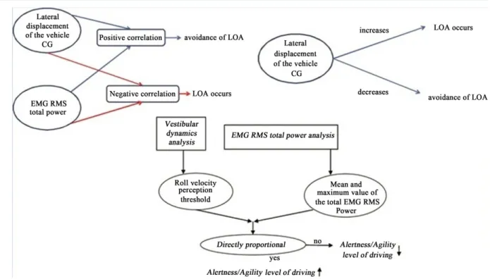
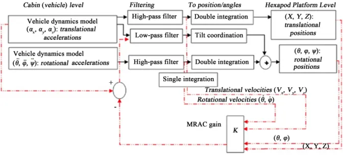
The proposed classical motion cueing algorithm’s sketch is indicated with continuous lines and arrows where the model reference controlled motion cueing algorithm’s sketch was drawn with discrete lines and arrows (Figure 1).
The proposed MRAC motion cueing algorithm here uses the same filters, gains (Figure 1 and Table 1) like used in the classical algorithm to compare the effects of the model reference adaptive control of the dynamic driving simulator. The main idea for Model Reference Adaptive Control (MRAC, which is also known as an
Table 1. Classical motion cueing algorithm parameters [25].
Symbol Longitudinal Lateral Roll Pitch Yaw
2nd order LP cut-off frequency (Hz) 0.3 0.7
2nd order LP damping factor 0.3 0.7
1st order LP time constant (s) 0.1 0.1 0.1
2nd order HP cut-off frequency (Hz) 0.5 0.5 2
2nd order HP damping factor 1 1 1
1st order HP time constant (s) 2 2 2
MRAS or Model Reference Adaptive System) is to build a closed-loop controller with parameters that can be updated to change the response of the system. The output of the system is compared to a desired response from a reference model. The control parameters are updated based on this error. The goal is for the parameters to converge to ideal values that cause the plant response to match the response of the reference model. It can focus on the continuous-time case and also on discrete-time design. A discrete-time MRAC was referred in this paper. The objective is to regulate the output minimized (platform-vehicle levels’ sensed acceleration difference minimization). The system (dynamic driving simulator) is subject to disturbances and is driven by controls [26]-[30].
Table 2 illustrates the constraints of the dynamic driving simulator SAAM, which was used in the real-time dll plugin in the SCANeR studio software for the both motion cueing algorithms. For the longitudinal, lateral and vertical displacements, the used gains were 0.2, 0.2 and 0.22 respectively.
The design step searches a state-feedback law that minimizes the cost function via applying this logic. Figure 2 illustrates the research method for the whole group of the subjects used in this article.
Both of the motion control algorithms (classical and MRAC) were integrated at the dynamic driving simulator SAAM with a “dll plugin” which were created with Microsoft Visual 2008 C++ used in SCANeR studio version 1.1.
2.2. Control Problem
We considered adiscrete-time MIMO (multiple-input multiple-output) system described by [27]-[30]
(
1)
( )
( ) ( )
,( )
x k+ = Ax k +Bu k y k =Cx k (1)
with n n
A∈ , × B∈n M× and M n
C∈ × being unknown and constant parameter matrices and x k
( )
∈n,( )
Mu k ∈ and y k
( )
∈M being the system state, input and output vector signals. 2.2.1. Control ObjectiveThe control objective is to design a state feedback control signal u(k) in Equation (1) such that all the closed- loop signals remain bounded and the system output signal y(k) tracks a given reference output ym
( )
k ∈Mthat is generated from the reference model system
( )
( ) ( )
m m
y k =W z r k (2)
Wm(z) is an M × M transfer matrix, and r(k), an M-dimensional real array, is a bounded reference input signal
[27] [30] [31]. 2.2.2. Assumptions
To begin the real-time controller design which is implemented in driving simulator as “dll plugin”, we assume
[27]:
(A1) All zeros of G zi
( )
C zIi(
Ai)
1B ii, 1, 2, ,N−
= − = lie within the unit circle in the z-plane;
Figure 2. Hypotheses: Our hypotheses are made up of three parts. 1) We stated that if the lateral displacement of the vehicle CG used inside the driving simulator and the power spent by arm muscles (from flexor carpi radialis) are positively corre-lated, it is an indicator of avoidance of LOA (LOC). Inversely, if they are negatively correcorre-lated, it is an objective metrics of occurrence of LOA. 2) We also declared that if the lateral displacement of the vehicle CG increases LOA occurs and in ad-verse case LOA decreases. 3) According to our third hypothesis, if the head (vestibular) level roll velocity perception thre-shold and the arm muscles power dissipation are positively correlated (cues conflict decrease) the alertness/agility level of the drivers increase too. We checked this criterion with respect to the real-time mean and maximum values of the total EMGRMS power measured from the arm muscles. Mean EMGRMS power is corresponding to the whole scenario whereas the
maximum value of the EMGRMS power is referring to the sudden change mostly depending on the sudden change of the road
curvatures, i.e. LOA. Table 2. Limits of each degree of freedom (DOF) for the SAAM driving simulator [25].
DOF Displacement Velocity Acceleration
Pitch ±22 deg ±30 deg/s ±500 deg/s2
Roll ±21 deg ±30 deg/s ±500 deg/s2
Yaw ±22 deg ±40 deg/s ±400 deg/s2
Heave ±0.18 m ±0.30 m/s ±0.5 g
Surge ±0.25 m ±0.5 m/s ±0.6 g
Sway ±0.25 m ±0.5 m/s ±0.6 g
and the reference system transfer matrix Wm
( )
zξ
m1( )
z−
= ;
(A3) All leading minors ∆j,j=1, 2,,M, of the high frequency gain matrix Kp are nonzero and their signs
are known.
2.2.3. State Feedback for State Tracking
For a state feedback for state tracking design, the controller structure is
( )
T( ) ( )
( ) ( )
1 2
where K k1
( )
∈n M× and K2( )
k ∈M M× are parameter matrices updated from some adaptive laws, so that the plant state vector signal x(k) can asymptotically track a reference state vector signal xm(k) generated from achosen reference system
(
1)
( )
( )
m m m m x k+ =A x k +B r k (4) where n n m A ∈ is stable and × n M mB ∈× . For such an adaptive control design, the matching conditions K1(k) and K2(k) are the estimates of the nominal K1
∗ and 2
K∗ which satisfy the conditions of matching
(
*T)
1 *( )
* 11 2 , 2
i i i i m P
C zI−A −B K − B K =W z K − =K (5) where KP =limz→∞ξm
( ) ( )
z G zi is the high frequency gain matrix of G z . The existence of i( )
K1∗ and K2∗is guaranteed under the nominal system condition: (A4) (A, B) is stabilizable and (A, C) is observable. 2.2.4. Tracking Error Equation
Substituting the control law Equation (3) in Equation (1), we obtain
(
)
(
*T)
( )
*( )
(
(
T( )
*T)
( )
(
( )
*)
( )
)
( )
( )
1 2 1 1 2 2
1 ,
x k+ = A+BK x k +BK r k +B K k −K x k + K k −K r k y k =Cx k (6)
In view of the reference model Equation (2), matching equations Equation (5) and Equation (6), the output tracking error e k
( )
=y k( )
−ym( )
k is( )
( )
( )
(
*T)
( )( )
1 T eA BK k 0 m P e k =W k +K θ ω k +C + x (7) where(
)
( )( )
*T 1 eA BK k 0C + x converges to zero exponentially and
( )
( )
* k kθ
=θ
−θ
(8)( )
( )
( )
T ( ) T 1 , 2 n M M k K k K k θ = ∈ + × (9) T * *T * 1 , 2 K K θ = (10)( )
T( ) ( )
T T , k x k r k ω = (11) 2.2.5. LDS DecompositionIn this section, we present the design and analysis of an adaptive scheme based on the LDS decomposition of the high frequency gain matrix KP.
To design an adaptive parameter update law, it is crucial to develop an error model in terms of some related parameter errors and the tracking error e k
( )
=y k( )
−ym( )
k .2.2.6. Error Model
Neglecting the term
(
)
( )( )
*T 1eA BK k 0
C + x , we obtain from Equation (7) and Equation (2)
( )
[ ]
( )
T( ) ( )
m z e k KP k k
ξ
=θ
ω
(12)To deal with the uncertainty of the high frequency gainmatrix KP, we use its LDS decomposition
P s s
K =L D S (13)
where S∈M M× with S=ST >0, Ls is an M × M unit triangular matrix, and
{
* * *}
[ ]
1 2 1 1
1
diag , , , diag sign , , sign M
s M M M D s s s γ γ − ∆ = = ∆ ∆ (14)
such that γ >i 0,i= 1, ,M , where γ is called adaptive gain, and
* 2
s is the second term in the diagonal of
the matrix Ds of the LDS decomposition [27] [28], substituting Equation (13) in Equation (12) yields
( )
[ ]
( )
( ) ( )
1 T
s m s
L−
ξ
z e k =D Sθ
kω
k (15)To parameterize the unknown Ls, θ0* is introduced in Equation (16)
* 21 * * 31 32 * 1 * 0 * 11 * * 1 1 0 0 0 0 0 0 , the dimension of is 0 0 0 M M s M M MM L I
θ
θ
θ
θ
θ
θ
θ
θ
− × − − = − = (16) Then, it yields (17):( )
[ ]
( )
*( ) ( )
T( ) ( )
0 m z e k m z e k D Ss k kξ
+θ ξ
=θ
ω
(17)A filter was designed h z
( )
=1 f z( )
, where f(z) is a stable monic polynomial of degree equals to the degree of ξm(z), operating both sides of Equation (17) by h(z)IM leads to( )
*T( )
*T( )
*T( )
( )
T( )
2 2 3 3 0, , , , M M s e k +θ η
kθ η
k θ η
k =D Sh z θ ω
k (18) where( )
m( ) ( )
[ ]
( )
1( )
, , M( )
e k =ξ
z h z e k = e k e k (19)( )
( )
( )
1 1 , , 1 , 2, , T i i k e k ei k R i M η − − = ∈ = (20)( )
( )
T * * * 1 1 , , 1 , 2, , i i i k ii k R i M θ θ θ − − = ∈ = (21)Based on this parameterized error equation, we reach the estimation error signal
( )
T( )
T( )
T( )
( ) ( )
( ) ( ) ( )
2 2 3 3
0, , , , M M
k k k k k k k k e k
ε
=θ η
θ η
θ η
+ψ
ξ
+ψ
ξ
+ (22)where θi
( )
k ,i=2, 3,,M are the estimates of *i
θ , and
ψ
( )
k −ψ
* are related parameter errors. 2.2.7. Adaptive LawsWithin the estimation error model Equation (22), the chosen adaptive laws [27]:
( )
( ) ( )( )
2 Γ , 2, 3, , i i k ik i k i M m k η θ θ = = (23)( )
( ) ( )
( )
T T 2 s D k k k m k ζ θ = − (24)( )
( ) ( )( )
T 2 k k k m k ξ ψ = −Γ (25)( )
T( ) ( )
T T , k x k r k ω = (26)where the signal
( )
k = 1( ) ( )
k ,2 k ,,M( )
k is computed from Equation (22), T 0, 2, 3, ,i
i i M
θ θ
Γ = Γ > =
and Γ = Γ >T 0 are adaptation gain matrices and
( )
T( ) ( )
T( ) ( )
(
T( ) ( )
)
1 2 21 iM i i
is a standard normalization signal, where ζ
( )
k =h z( )[ ]( )
ω k [27].3. Methods
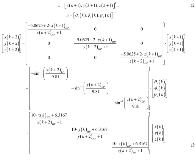
We consider the dynamic model of the hexapod simulator described by Equation (28) which is a three state va-riable (x). The control inputs are (u) the pitch angle (θv), the roll angle (ϕv) and the yaw angle (ψv) of the vehicle model. Our MRAC model was given in Equation (29) (HP: high pass filtered motion, LP: low pass filtered mo-tion) which was with a sampling interval of T = 1/60 seconds to obtain the discrete-time motion cueing algo-rithms implemented in our dll plugin.
(
) (
) (
)
T 1 , 1 , 1 , x=x k+ y k+ z k+ (28)( ) ( )
( )
T , , v v v u= θ k φ k ψ k (
)
(
)
(
)
(
)
(
)
(
)
(
)
(
)
(
)
(
)
(
)
(
)
(
)
(
)
1 1 1 5.0625 2 1 2 1 2 1 5.0625 2 1 2 1 2 1 2 1 5.0625 2 1 2 1 2 sin 9.81 2 sin 9 0 0 0 0 0 .81 s 0 in HP HP HP HP HP HP LP LP x k x k x k x k y k y k y k y k z k z k z k z k x k y k z − − − − + ⋅ + + + + − + ⋅ + + + ⋅ + + + + + − + ⋅ + = + + + − + − − +(
)
( )
( )
( )
( )
(
)
( )
(
)
( )
(
)
( )
( )
( )
2 9.81 10 6.3167 2 1 10 6.3167 2 1 10 6.3167 2 1 v v v LP HP HP HP HP HP HP k k k k x k x k x k y k y k y k z k z k z k θ φ ψ + ⋅ + + + ⋅ + ⋅ − ⋅ + + ⋅ + + + (29)3.1. Subjects
Twenty-six healthy participants took place in the experiments (4 females, 22 males) with a mean age of 28.9 ± 5.8 years old and a driving license holding with a mean experience of 9.7 ± 6.6 years.
3.2. Protocol
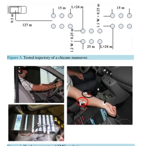
Figure 3 shows the trajectory of the chicane maneuver that we used in this experiment protocol (Here W = 1 m and L = 1.5 m). The vehicle velocity during the simulator experiments was chosen as constant at 60 km/h. The same scenario was driven at the classical and the MRAC motion cueing algorithms in order to compare the bio-mechanical interactions (head level dynamics and vehicle level dynamics interaction, neuromuscular dynamics and vehicle level dynamics and lastly head level dynamics and neuromuscular dynamics) of the participants.
Vestibular level dynamics of the participants refer to the head movements of them (see Figure 4). It was measured via a XSens motion tracking sensor. Vehicle level dynamics indicate the visual cues which come from the surroundings of the vehicle when it is driven at the simulator as real-time.
Figure 3. Tested trajectory of a chicane maneuver.
Figure 4. Head movement and EMG analysis.
3.3. Data Analysis
Multi-level data acquisition was performed at two levels as follows: 3.3.1. Vestibular Level Data Acquisition (through Sensor)
Such as the roll, pitch, yaw angles and rates as well as the accelerations in X,Y and Z. Quaternions have been used, since they are simpler to compose and to avoid singularity for angular calculations, so-called the problem of gimbal lock compared to Euler angles. The application domains of quaternions can be counted as computer graphics, computer vision, robotics, navigation, flight dynamics [32] and orbital mechanics of satellites [33]. Because we have dealt with the hexapod driving simulator in real-time, we have used quaternions. The data are calibrated due to three dimensional quaternion orientation.The sampling rate for the data registration during the sensor measurements is 20 Hz. For the calibrated data acquisition, the alignment reset has been chosen which simply combines the object and the heading resets at a single instant in time. This has the advantage that all co‐ ordinate systems can be aligned with a single action.
3.3.2. Electromyography (via Biopac System)
Electromyography (EMG) is an evaluation method of the electrical activity produced by musculoskeletal system. EMG is performed using an instrument called an electromyograph, to realize a record called an electromyogram. An electromyography detects the electrical potential generated by muscle cells [34] when these cells are electri-cally or neurologielectri-cally activated. The signals can be analyzed to detect and identify medical abnormalities, mus-cle activation level, and recruitment order or to analyze the biomechanics of human or animal movements [34].
By using the Biopac systems, several frequency and time domain techniques could be used for data reduction of EMG signals [21].
For this study, it was chosen to deal with the EMGRMS (root mean square: which is a product of longitudinal,
to investigate their associations with RVT (˚/s in unit, which is an indicator of the conflict in dynamics). - EMGRMS mean total power yields the average power of the power spectrum within the epoch [21].
- EMGRMS total power is equal to the sum of power at all frequencies of the power spectrum within the epoch
[21].
- Epoch corresponds to how many time steps (∆t) a whole time series signal is divided into [21].
For the calibration of the electromyography, a gain of 1000 was used. And the Figure 4 depicts the data ac-quisition during the experiments; the electrical activities of the muscles were registered by a non-invasive sur-face EMG method through two analog channels. The signals were collected with 10 Hz for low cut-off, 500 Hz for high cut-off frequencies (a band-pass filter with a frequency range: 10 - 500 Hz).
Electrodes in black circle were connected to flexor carpi radialis muscle where the electrodes in red circle were connected to brachioradialis muscles. We measured and saved the electrical activity changes on the bra-chioradialis and flexor carpi radialis muscles. In this paper, we explained the results which were taken from the muscle ‘flexor carpi radialis’ (at right hand side, Figure 4).
4. Results and Discussion
4.1. Vestibular and Neuromuscular Dynamics Interaction with Vehicle Dynamics
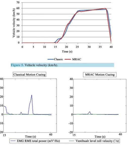
Figure 5 corresponds to the vehicle velocity during the experiments with driver for the EMG-RV analysis done in Figure 6.
Figure 5. Vehicle velocity (km/h).
Figure 6 indicates a real-time measurement of EMGRMS total power-head roll velocity for one out of the
twenty six subjects who participated in the experiments.
If Figure 3, Figure 5 and Figure 6 are evaluated together it is possible to characterize the neuromuscular dy-namics (via EMG analysis), vestibular dydy-namics more clearly.
It can be seen that the discrepancy has been decreased between the EMGRMS total power and the roll velocity
at vestibular level by using MRAC motion cueing (see Figure 6). This figure also proves less contradicting cues from the arm muscular and the vestibular dynamics system, in other words less LOA (loss of adhesion) of the vehicle or more agility and alertness levels of the driver in the lateral dynamics.
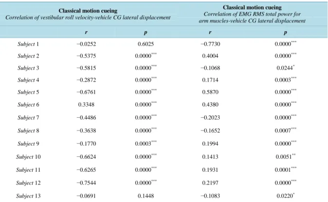
Table 3 summarizes the correlation of the arm muscle (flexor carpi radialis) power and the head level roll ve-locity from a sensor attached to the right ear of the drivers via a headphone (Figure 4) with the vehicle CG (center of gravity) lateral displacement for the classical motion cueing algorithm situation. From Table 3, it is seen that there have been significant correlation between vestibular roll velocity and vehicle CG lateral dis-placement except for Subject 1 and Subject 13. Furthermore, merely the subject 6 has yielded a positive correla-tion between the vestibular level roll velocity and the arm muscles power. Apart from subject 6, they have dem-onstrated a negative correlation, which actually represents an increased level of the visuo-vestibular cue conflict. According to Table 3, it can be concluded that there have been significant correlations between arm muscle powers and vehicle CG lateral displacements for all the thirteen subjects at the classical motion cueing case. Moreover, a negative correlation has been resulted between the arm muscles power and the vehicle CG lateral displacements for the subjects 1, 3, 7, 8 and 13 for the classical algorithm, whereas a positive correlation has been obtained for the rest of the subjects. These correlations show us that for the 8 subjects the vehicle has been driven with the less controlloss out of the 13 subjects.
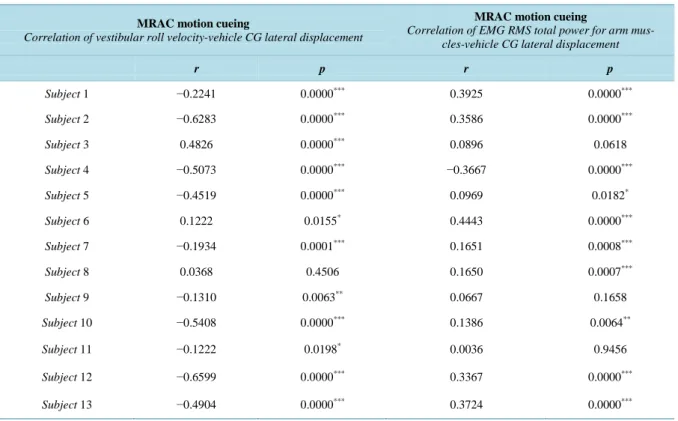
Table 4 gives the correlation of the arm muscle (flexor carpi radialis) power and the head level roll velocity with the vehicle CG (center of gravity) lateral displacement for the MRAC motion cueing algorithm case. From Table 4, it can be seen that there have been significant correlation between vestibular roll velocity and vehicle CG lateral displacement except for Subject 8. Furthermore, the subject 3, 6 and 8 have yielded a positive corre-lation between the vestibular level roll velocity and the arm muscles power. Apart from these subjects, they have demonstrated a negative correlation.
Table 3. Vestibular-arm muscle dynamics interaction for classical motion cueing.
Classical motion cueing
Correlation of vestibular roll velocity-vehicle CG lateral displacement
Classical motion cueing
Correlation of EMG RMS total power for arm muscles-vehicle CG lateral displacement
r p r p Subject 1 −0.0252 0.6025 −0.7730 0.0000*** Subject 2 −0.5375 0.0000*** 0.4004 0.0000*** Subject 3 −0.5815 0.0000*** −0.1068 0.0244* Subject 4 −0.2872 0.0000*** 0.1714 0.0003*** Subject 5 −0.6761 0.0000*** 0.5870 0.0000*** Subject 6 0.3348 0.0000*** 0.4380 0.0000*** Subject 7 −0.4486 0.0000*** −0.2023 0.0000*** Subject 8 −0.3638 0.0000*** −0.1652 0.0007*** Subject 9 −0.1770 0.0003*** 0.1994 0.0000*** Subject 10 −0.6624 0.0000*** 0.1413 0.0051** Subject 11 −0.6265 0.0000*** 0.1931 0.0001*** Subject 12 −0.7544 0.0000*** 0.2197 0.0000*** Subject 13 −0.0691 0.1448 −0.1083 0.0220* *
Table 4. Vestibular-arm muscle dynamics interaction for MRAC motion cueing.
MRAC motion cueing
Correlation of vestibular roll velocity-vehicle CG lateral displacement
MRAC motion cueing
Correlation of EMG RMS total power for arm mus-cles-vehicle CG lateral displacement
r p r p Subject 1 −0.2241 0.0000*** 0.3925 0.0000*** Subject 2 −0.6283 0.0000*** 0.3586 0.0000*** Subject 3 0.4826 0.0000*** 0.0896 0.0618 Subject 4 −0.5073 0.0000*** −0.3667 0.0000*** Subject 5 −0.4519 0.0000*** 0.0969 0.0182* Subject 6 0.1222 0.0155* 0.4443 0.0000*** Subject 7 −0.1934 0.0001*** 0.1651 0.0008*** Subject 8 0.0368 0.4506 0.1650 0.0007*** Subject 9 −0.1310 0.0063** 0.0667 0.1658 Subject 10 −0.5408 0.0000*** 0.1386 0.0064** Subject 11 −0.1222 0.0198* 0.0036 0.9456 Subject 12 −0.6599 0.0000*** 0.3367 0.0000*** Subject 13 −0.4904 0.0000*** 0.3724 0.0000*** *
Means one zero after the point “.”, **means two zeros after the point “.”, ***means three and more than three zeros after the point “.”.
According to Table 4, it can be concluded that there have been significant correlations between arm muscle powers and vehicle CG lateral displacements apart from the subjects 3, 9 and 11 at the MRAC motion cueing condition. Moreover, a negative correlation has been coincided between the arm muscles power and the vehicle CG lateral displacements only for the subject4 for the MRAC algorithm, whereas a positive correlation has been occurred for the rest of the subjects. These correlations show us that only for the 1subject (subject 4) the vehicle has been driven with a propensity of control loss out of the 13 subjects, when uniquely the correlation between the arm muscles power and the vestibular level roll velocity are taken into account.
From Table 3, Table 4 and Figure 7, it is seen that loss of adhesion (LOA) of the vehicle causes a visuo- vestibular cues conflict (if the correlation of vestibular roll velocity with vehicle CG lateral displacement is neg-ative) however visuo-vestibular conflict is not always followed by a LOA (if the correlation of EMGRMS total
power with vehicle CG lateral displacement is negative).
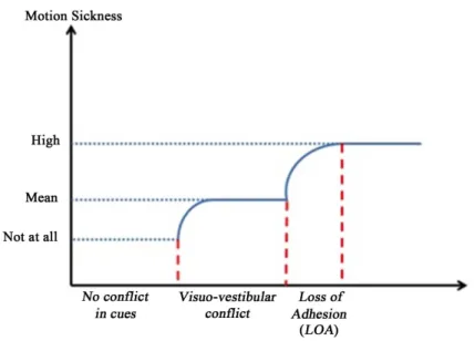
Figure 8 summarizes our findings about the relationships of multi sensory (vestibular, neuromuscular, vehicle (visual)) cues with motion sickness incidence as a metrics for lateral dynamics in terms of sensory cue conflict theory [35] [36] depending on Table 3 and Table 4 respectively for this study. According to this figure; when there is no conflict at all in cues, no motion sickness is occurred. As there is visuo-vestibular cue conflict, it results as a moderate level of motion sickness. Eventually when LOA is observed, the motionsickness gets higher levels.
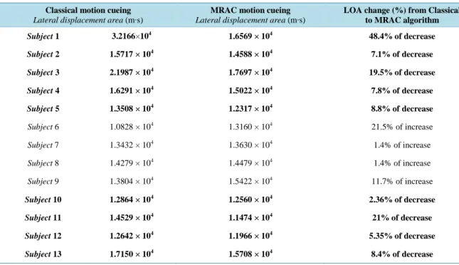
Table 5 illustrates the lateral displacement area (Equation (30) in m·s) [19] [20] [37] (see Figure 9) under the vehicle CG lateral displacement (YCG) from the time series graphs where t is time
Lateral displacement area=
∫
otYCGdt (30)According to Table 5, it can be summed up that apart from the subjects 6, 7, 8 and 9 the loss of adhesion has decreased; in other words agility or alertness level of the drivers have increased for the classical algorithm com-paring to MRAC algorithm which make the vehicle maintain on the desired route. In contrast for the rest of the subjects, the agility level of the drivers has increased, in other words LOC of the vehicle has decreased with MRAC motion cueing. For the subjects 6, 7, 8 and 9 (4 subjects out of 13 subjects) the classical motion cueing algorithm had the higher level of loss of control (LOC) of the vehicle in the dynamic driving simulator. For the
Figure 7. Vestibular-neuromuscular-vehicle dynamics interaction.
Figure 8. Relationships of multi sensory cues conflict with motion sickness.
Figure 9. Lateral displacement area.
rest of the subjects (9 subjects out of 13 subjects), the MRAC motion cueing algorithm brought a more controll-able vehicle in the dynamic simulator as operated in real-time. This shows that the MRAC motion cueing algo-rithm (closed loop control) provides a less LOA and LOC comparing to the classical motion cueing algoalgo-rithm (open loop control).
Table 5. Lateral displacement area for both algorithms.
Classical motion cueing
Lateral displacement area (m∙s)
MRAC motion cueing
Lateral displacement area (m∙s)
LOA change (%) from Classical to MRAC algorithm Subject 1 3.2166×10⁴ 1.6569 × 10⁴ 48.4% of decrease Subject 2 1.5717 × 10⁴ 1.4588 × 10⁴ 7.1% of decrease Subject 3 2.1987 × 10⁴ 1.7697 × 10⁴ 19.5% of decrease Subject 4 1.6291 × 10⁴ 1.5022 × 10⁴ 7.8% of decrease Subject 5 1.3508 × 10⁴ 1.2317 × 10⁴ 8.8% of decrease Subject 6 1.0828 × 10⁴ 1.3160 × 10⁴ 21.5% of increase Subject 7 1.3432 × 10⁴ 1.3630 × 10⁴ 1.4% of increase Subject 8 1.4279 × 10⁴ 1.4479 × 10⁴ 1.4% of increase Subject 9 1.3804 × 10⁴ 1.5422 × 10⁴ 11.7% of increase Subject 10 1.2864 × 10⁴ 1.2560 × 10⁴ 2.36% of decrease Subject 11 1.4529 × 10⁴ 1.1474 × 10⁴ 21% of decrease Subject 12 1.2642 × 10⁴ 1.1966 × 10⁴ 5.35% of decrease Subject 13 1.7150 × 10⁴ 1.5708 × 10⁴ 8.4% of decrease
4.2. Vestibular and Neuromuscular Dynamics Interaction
After having completed the data evaluation by individual as above, the overall data analysis has been studied for the thirteen subject group for each motion cueing (both for the classical and the MRAC motion cueing algo-rithms).
The overall data analysis was done by using a two-way ANOVA (Analysis of Variance) and Pearson’s corre-lation with an α = 0.05. In order to accomplish the statistical analysis, we took
- the vestibular roll velocity into account, which were measured from the right ear level of the participants during the real-time simulator experiments through the motion tracking sensor.
- the EMGRMS total power from the muscle ‘flexor carpi radialis’.
The two-way ANOVA was applied to identify the level of significance as between subjects’ principle test. The Pearson’s correlation was computed to clarify the correlation of the vestibular level roll velocity threshold with the EMGRMS power dissipation of the arm muscles.
4.2.1. Two-Way ANOVA
The two-way ANOVA tests were used to check the influence of one type of response dynamics (spent power from the arms) of the drivers on the other type of response dynamics (vestibular roll velocity) of them as an in-teraction metrics.
By studying the output of the two-way ANOVA for the proposed classical motion cueing algorithm, we see that there is no evidence of a significant interaction effect (F = 3.74, p = 0.085 > 0.05) between those two types of response dynamics of the drivers. We therefore can conclude that no interaction was obtained between the EMGRMS mean power and the vestibular roll velocity threshold. The test for the main effect of the vestibular roll
velocity perception threshold (F = 45.17, p < 0.0001) shows a significant roll velocity perception threshold ef-fect on the EMGRMS maximum power level. Finally, the test for the main effect of the EMGRMS mean power (F =
1360.89, p < 10−9) tells us there is an evidence to conclude that the EMGRMS mean power has a significant effect
on the EMGRMS maximum power level.
By investigating the output of the two-way ANOVA for the proposed model reference adaptive control mo-tion cueing algorithm, we see that there is no evidence of a significant interacmo-tion effect (F = 0.43, p = 0.528 > 0.05) between those two types of response dynamics of the drivers. We therefore cannot conclude that an inte-ractionis found between the EMGRMS mean power and the roll velocity threshold. The test for the main effect of
perception threshold effect on the EMGRMS maximum power level. Finally, the test for the main effect of the
EMGRMS mean power (F = 232.44, p < 10−6) tells us there is an evidence to conclude that the EMGRMS mean
power has a significant effect on the EMGRMS maximum power level.
4.2.2. Pearson’s Correlation
Having searched the relationships of the roll velocity thresholds with the EMGRMS mean and maximum total
power, we recognized that if we drive the same scenario with the MRAC, it shows a more alerted (agile) mode compared to the classical motion cueing algorithm. Because, the correlation coefficients (r) between the roll ve-locity thresholds and the EMGRMS mean/maximum total power are positive for the MRAC and negative for the
classical motion cueing algorithm.
We described the RV (roll velocity) at “vestibular” level [5] [6] [19] [20]. MATLAB/Simulink applications were used to process the RVT data (maximum head level roll velocity at low frequent motion independent from
the direction): Vestibular level roll velocity signals were conditioned with a 1st order Butterworth low-pass filter
at 5 Hz.
Root-mean square (RMS) of EMG (EMGRMS) (mV) values were computed based on a total range of motion
during the driving phase of the simulator experiments [18] [29], using the following Equation (31):
( )
2 1 EMGRMS tt TEMG t dt T + =∫
(31)where t is the onset of signal time and T is the duration of RMS averaging [38].
For the frequency domain analysis used in this study to determine the spent power/energy by the arm muscles of the drivers, a Fast Fourier Transformation algorithm was used to calculate the power spectrum of EMG sig-nals (mV) [34] [38] with the following Equation (32):
( )
( )
2n
PSD f = FFT x (32)
where xn is a set of consecutive EMG signals with the specific number of epochs, PSD is power spectral density
in mV2/Hz [34] [38]. In this article:
- EMGRMS total power indicates the dissipated power (times series data) during the driving simulation
experi-ments (Equation (31) and Equation (32)). It yields the sum of the power at all frequencies of the power spec-trum within the epoch.
- EMGRMS maximum total power refers to the peak values (one value point) obtained from the dissipated
energy during the driving simulation experiments (Equation (31) and Equation (32)).
- EMGRMS mean total power indicates the mean of the sum of the dissipated power (one value point) at all
frequencies during the driving simulation experiments (Equation (31) and Equation (32)).
- Roll velocity perception threshold gives maximum vestibular level roll velocityat low frequent motion
inde-pendent from the direction: Those signals were conditioned with a 1st order Butterworth low-pass filter at 5
Hz.
Figure 10 and Figure 11 illustrate the difference of the both motion cueing algorithms in terms of RVT (˚/s) to EMGRMS maximum total power (mV2/Hz) as well as to EMGRMS mean total power (mV2/Hz) changes. In
or-der to assess the relationships, we used MATLAB. The vertical axes were illustrated in the logarithmic scale in order to show the data points better.
Due to Figure 12, it is clearly seen that some of the participants reached extreme outliers (red stars) in terms of roll velocity thresholds by driving the classical motion cueing algorithms while the RVT for the MRAC mo-tion cueing algorithm showed no extreme outliers. In addimo-tion, the discrepancy of the RVT for classical momo-tion cueing algorithm (from −3.1˚/s to 2.4˚/s, it makes a discrepancy of 5.5˚/s) is greater than the one (from −0.8˚/s to 1.1˚/s, it makes a discrepancy of 1.9˚/s) in MRAC motion cueing algorithm, which also specifies a higher level of vestibular sensory conflict.
According to Pearson’s correlation, it is shown that the RVT and the EMGRMS mean power are positively
cor-related (r = 0.228, p = 0.453) for the MRAC algorithm and they are negatively corcor-related (r = −0.167, p = 0.586) for the classical algorithm.
Figure 10. RVT and EMG RMS maximum total power analysis relationships for all subjects.
Figure 11. RVT and EMG RMS mean total power analysis relationships for all subjects.
Figure 12. RVT comparison for the classical and the MRAC motion cueing algorithms for all subjects.
correlated (r = 0.192, p = 0.531) for the MRAC motion cueing algorithm and they are negatively correlated (r = −0.178, p = 0.560) for the classical motion cueing algorithm. (Figure 10 and Figure 11).
5. Conclusion
Head roll velocity, arm muscle and vehicle dynamics interaction were investigated. For the classical motion cueing the discrepancy of the curves (vestibular-arm muscle dynamics) has increased (see Figure 6).
Conclud--4 -3 -2 -1 0 1 2 3 0 0.5 1 1.5 2 2.5x 10 -5
Roll velocity perception threshold (°/s)
E M G R M S M a x im u m T o ta l P o w er ( V 2 /Hz ) Classical algorithm MRAC algorithm -4 -3 -2 -1 0 1 2 3 0 0.5 1 1.5 2x 10 -6
Roll velocity perception threshold (°/s)
E M G R M S M ea n T o ta l P o w er ( V 2 /Hz ) Classical algorithm MRAC algorithm -3 -2 -1 0 1 2 3 R o ll v el o ci ty p er ce p ti o n t h re sh o ld ( °/ s) Classical algorithm -3 -2 -1 0 1 2 3 R o ll v el o ci ty p er ce p ti o n t h re sh o ld ( °/ s) MRAC algorithm
ing up from Table 5; 9 out of the 13 subjects have obtained a lower amount of surface according to the lateral displacement of the vehicle CG with the MRAC algorithm. This indicates an improvement in LOA (loss of ad-hesion) at the MRAC motion cueing comparing to the classical motion cueing (69.2% of decrease in LOA, 30.8 % of increase in LOA). Due to Table 3, 5 out of 13 subjects have shown a propensity on LOA and decrease in agility/alertness level of the drivers at the classical algorithm (proximity to a LOA incidence is 38.5%). Table 4 has illuminated an inclination to an incidence of LOA for merely 1 subject (propensity to a LOA is 7.7%).
We also investigated the vestibular sensed roll velocity perception threshold (impulse effect dynamics: high frequent motion) with the total power spent by the arm muscles. It gave an idea about the driver’s behaviours as “alertness (agility)”.
Having a closed loop control of the hexapod platform (a MRAC motion cueing strategy) supplied more alert-ness (39.5% increase in agility: r = 0.228, p = 0.453 for the MRAC algorithm and r = −0.167, p = 0.586 for the classical algorithm in terms of RVT-EMGRMS mean total power. And also 37% increase in agility: r = 0.192, p =
0.531 for the MRAC algorithm and r = −0.178, p = 0.560 for the classical algorithm in terms of RVT-EMGRMS
maximum total power), that helps the dynamic simulator be driven more controllably, compared to an open loop control of the hexapod platform (a classic motion cueing strategy) with the same filters and gains (Figure 1 and Table 1).
We thus cannot conclude that there is an interaction between the EMGRMS means power and the roll velocity
threshold. The test for the main influence of the vestibular roll velocity perception threshold indicates a signifi-cant roll velocity perception threshold influence on the EMGRMS maximum power level. Eventually, the test for
the main effect of the EMGRMS mean power gives us an evidence to conclude that there is a significant EMGRMS
mean power effect on the EMGRMS maximum power level for both classical and MRAC motion cueing
algo-rithms.
As a conclusion, the MRAC motion cueing strategy optimized the dynamic simulator condition with respect to the classical motion cueing strategy, so that it resulted as an improved situation for the drivers in terms of the “avoidance of LOA” and improving the “motion sickness” depending on sensory conflict theory between neu-romuscular-vehicle (visual) cues, between vestibular-vehicle (visual) cues.
It also proved that the neuromuscular-vehicle dynamics conflict has influence on visuo-vestibular conflict; however, the visuo-vestibular cue conflict does not influence the neuromuscular-vehicle dynamics interactions.
As prospective work, we would like to evaluate the sickness regarding the pitch velocity/acceleration percep-tion threshold as well as the neuromuscular-vestibular reacpercep-tion time relapercep-tionships of the drivers on various road scenarios, under different controls of the hexapod platform with correlations in inertial, vestibular, neuromuscu-lar cues.
Acknowledgements
Arts et Métiers Paris Tech built up the SAAM driving simulator with the partnership of Renault.
References
[1] Angelaki, D.E., Gu, Y. and DeAngelis, G.C. (2009) Multisensory Integration: Psychophysics, Neurophysiology, and Computation. Current Opinion in Neurobiology, 19, 452-458. http://dx.doi.org/10.1016/j.conb.2009.06.008
[2] Aykent, B., Paillot, D., Merienne, F., Fang, Z. and Kemeny, A. (2011) Study of the Influence of Different Washout Algorithms on Simulator Sickness for Driving Simulation Task. Proceedings of the ASME 2011 World Conference on
Innovative Virtual Reality WINVR2011, Milan, 331-341. http://dx.doi.org/10.1115/WINVR2011-5545
[3] Chen, D., Hart, J. and Vertegaal, R. (2007) Towards a Physiological Model of User Interruptability. IFIP International
Federation for Information Processing, INTERACT 2007, 439-451.
[4] Dichgans, J. and Brandt, T. (1973) Optokinetic Motion Sickness and Pseudo-Coriolis Effects Induced by Moving Vis-ual Stimuli. Acta Otolaryngologica, 76, 339-348. http://dx.doi.org/10.3109/00016487309121519
[5] DiZio, P. and Lackner, J.R. (1989) Perceived Self-Motion Elicited by Postrotary Head Tilts in a Varying Gravitoiner-tial Force Background. Perception & Psychophysics, 46, 114-118. http://dx.doi.org/10.3758/BF03204970
[6] Nehaoua, L., Arioui, H., Espié, S. and Mohellebi, H. (2006) Motion Cueing Algorithms for Small Driving Simulator.
IEEE International Conference in Robotics and Automation (ICRA06), Orlando.
[7] Kemeny, A. (2014) From Driving Simulation to Virtual Reality. Proceedings of the 2014 Virtual Reality International
[8] Benson, A.J., Hutt, E.C. and Brown, S.F. (1989) Thresholds for the Perception of Whole Body Angular Movement about a Vertical Axis. Aviation, Space, and Environmental Medicine, 60, 205-213.
http://psycnet.apa.org/psycinfo/1989-21186-001
[9] Guedry Jr., F.E. (1964) Visual Control of Habituation to Complex Vestibular Stimulation in Man. Bureau of Medicine and Surgery, Project MR005.13-6001, Subtask 1 Report No. 95, NASA Order No. R-93, US Naval School of Aviation Medicine, US Naval Aviation Medical Center, Pensacola, 1-16.
http://informahealthcare.com/doi/abs/10.3109/00016486409121398
[10] Guedry, F.E. and Montague, E.K. (1961) Quantitative Evaluation of the Vestibular Coriolis Reaction. Aviation, Space,
and Environmental Medicine, 32, 487-500. http://eurekamag.com/research/025/329/025329418.php
[11] Wiederhold, B.K. and Bouchard, S. (2014) Sickness in Virtual Reality. Advances in Virtual Reality and Anxiety
Dis-orders, 35-62. http://dx.doi.org/10.1007/978-1-4899-8023-6_3
[12] DiZio, P. and Lackner, J.R. (1988) The Effects of Gravitoinertial Force Level and Head Movements on Post-Rotational Nystagmus and Illusory After-Rotation. Experimental Brain Research, 70, 485-495.
http://dx.doi.org/10.1007/BF00247597
[13] Kolasinski, E.M. (1995) Simulator Sickness in Virtual Environments. Army Project Number 2O262785A791, Educa-tion and Training Technology.
[14] Asadi, H., Mohammadi, A., Mohamed, S. and Nahavandi, S. (2014) Adaptive Translational Cueing Motion Algorithm Using Fuzzy Based Tilt Coordination. Neural Information Processing, Springer International Publishing, Berlin, 474- 482.
[15] Curry, R., Artz, B., Cathey, L., Grant, P. and Greenberg, J. (2002) Kennedy SSQ Results: Fixed- vs Motion-Based FORD Simulators. Proceedings of Driving Simulation Conference, Paris, 11-13 September 2002, 289-300.
[16] Kim, M.S., Moon, Y.G., Kim, G.D. and Lee, M.C. (2010) Partial Range Scaling Method Based Washout Algorithm for a Vehicle Driving Simulator and Its Evaluation. International Journal of Automotive Technology, 11, 269-275. http://dx.doi.org/10.1007/s12239-010-0034-0
[17] MOOG FCS, 6 DOF Motion System (2006) Motion Drive Algorithm (MDA) Software Tuning Manual Version 1.0. Document No: LSF-0468, Revision: A.
[18] Siegler, I., Reymond, G., Kemeny, A. and Berthoz, A. (2001) Sensorimotor Integration in a Driving Simulator: Con-tributions of Motion Cueing in Elementary Driving Tasks. Proceedings of Driving Simulation Conference, Sophia- Antipolis, 5-7 September 2001, 21-32.
[19] Meywerk, M., Aykent, B. and Tomaske, W. (2009) Einfluss der Fahrdynamik-regelung auf die Sicherheit von N1- Fahrzeugen bei unterschiedlichen Bela-dungszuständen. Teil 1: Grundlagen, Unfallstatistik, Abstütz- und Beladungs- einrichtung, Fahrzeugdatenermittlung. FE 82.329/2007.
http://bast.opus.hbz-nrw.de/frontdoor.php?source_opus=354&la=de
[20] Meywerk, M., Aykent, B. and Tomaske, W. (2009) Einfluss der Fahrdynamik-regelung auf die Sicherheit von N1- Fahrzeugen bei unterschiedlichen Bela-dungszuständen. Teil 2: Fahrversuche und Fahrsimulatorversuche. FE 82.329/ 2007. http://bast.opus.hbz-nrw.de/frontdoor.php?source_opus=355&la=de
[21] AcqKnowledge® 4 (2011) Software Guide For Life Science Research Applications, Data Acquisition and Analysis with BIOPAC MP Systems Reference Manual for AcqKnowledge® 4.2 Software &MP150 or MP36R Hardware/ Firmware on Windows® 7 or Vista or Mac OS® X 10.4-10.6. 357-358.
[22] Benson, A.J. (1990) Sensory Functions and Limitations of the Vestibular Systems. In: Warren, R. and Wertheim, A.H., Eds., Perception and Control of Self-Motion, Laurence Erlbaum Associates, Hinsdale, 145-170.
[23] Kemeny, A. and Panerai, F. (2003) Evaluating Perception in Driving Simulation Experiments. Trends in Cognitive
Sciences, 7, 31-37. http://dx.doi.org/10.1016/S1364-6613(02)00011-6
[24] Pick, A.J. (2004) Neuromuscular Dynamics and the Vehicle Steering Task. Ph.D. Dissertation, St Catharine’s College, Cambridge University Engineering Department, Cambridge.
[25] Aykent, B., Merienne, F., Paillot, D. and Kemeny, A. (2013) Influence of Inertial Stimulus on Visuo-Vestibular Cues Conflict for Lateral Dynamics at Driving Simulators. Journal of Ergonomics, 3, 1-7.
http://omicsgroup.org/journals/influence-of-inertial-stimulus-on-visuo-vestibular-cues-conflict-for-lateral-dynamics-at-driving-simulators-2165-7556.1000113.pdf
[26] Duarte, M.A. and Ponce, R.F. (1997) Discrete-Time Combined Model Reference Adaptive Control. International
Journal of Adaptive Control and Signal Processing, 11, 501-517.
http://dx.doi.org/10.1002/(SICI)1099-1115(199709)11:6<501::AID-ACS448>3.0.CO;2-G
[27] Guo, J., Liu, Y. and Tao, G. (2009) Multivariable MRAC with State Feedback for Output Tracking. American Control
Conference, Hyatt Regency Riverfront, PaperWeA18.5, St. Louis, 10-12 June 2009, 592-597.
[29] Maiti, D., Guo, J. and Tao, G. (2011) A Discrete-Time Multivariable State Feedback MRAC Design with Application to Linearized Aircraft Models with Damage. American Control Conference, San Francisco, 29 June-1 July 2011, 606-611.
[30] Tao, G. and Ioannou, P.A. (1993) Model Reference Adaptive Control for Plants with Unknown Relative Degree. IEEE
Transactions on Automatic Control, 38, 976-982. http://dx.doi.org/10.1109/9.222314 [31] Tao, G. (2003) Adaptive Control Design and Analysis. John Wiley and Sons, New York.
http://dx.doi.org/10.1002/0471459100
[32] Katz, A. (1996) Computational Rigid Vehicle Dynamics. Krieger Publishing Co., Malabar.
[33] Kuipers, J.B. (1999) Quaternions and Rotation Sequences: A Primer with Applications to Orbits, Aerospace, and Vir-tual Reality. Princeton University Press, Princeton.
[34] Mesh Electromyography (2015) National Library of Medicine—Medical Subject Headings, Mesh. http://www.ncbi.nlm.nih.gov/mesh/68004576
[35] Oman, C. (1989) Sensory Conflict in Motion Sickness: An Observer Theory Approach. NASA, Ames Research Center, Spatial Displays and Spatial Instruments, 15 p.
[36] Oman, C. (1990) Motion Sickness: A Synthesis and Evaluation of the sensory Conflict Theory. Canadian Journal of
Physiology and Pharmacology, 68, 294-303. http://dx.doi.org/10.1139/y90-044
[37] Electronic Code of Federal Regulations (2015) Title 49: Transportation Part 571—Federal Motor Vehicle Safety Stan-dards Subpart B—Federal Motor Vehicle Safety StanStan-dards § 571.126 Standard No. 126; Electronic Stability Control Systems. US Government Printing Office, Electronic Code of Federal Regulations.
http://www.ecfr.gov/cgi-bin/text-idx?SID=6099cd0521e2251f35642c554b1c3001&node=pt49.6.571&rgn=div5#se49. 6.571_1126
[38] Fu, W., Liu, Y., Zhang, S., Xiong, X.J. and Wei, S.T. (2012) Effects of Local Elastic Compression on Muscle Strength, Electromyographic, and Mechanomyographic Responses in the Lower Extremity. Journal of Electromyography and
![Table 1. Classical motion cueing algorithm parameters [25].](https://thumb-eu.123doks.com/thumbv2/123doknet/7414602.218519/5.892.145.807.145.329/table-classical-motion-cueing-algorithm-parameters.webp)