HAL Id: hal-01018700
https://hal.archives-ouvertes.fr/hal-01018700
Submitted on 4 Jul 2014
HAL is a multi-disciplinary open access
archive for the deposit and dissemination of
sci-entific research documents, whether they are
pub-lished or not. The documents may come from
teaching and research institutions in France or
abroad, or from public or private research centers.
L’archive ouverte pluridisciplinaire HAL, est
destinée au dépôt et à la diffusion de documents
scientifiques de niveau recherche, publiés ou non,
émanant des établissements d’enseignement et de
recherche français ou étrangers, des laboratoires
publics ou privés.
Network-based correlated correspondence for
unsupervised domain adaptation of hyperspectral
satellite images
Julien Rebetez, Devis Tuia, Nicolas Courty
To cite this version:
Julien Rebetez, Devis Tuia, Nicolas Courty. Network-based correlated correspondence for
unsuper-vised domain adaptation of hyperspectral satellite images. International Conference on Pattern
Recog-nition (ICPR 2014), Aug 2014, Stockholm, Sweden. pp.1–6. �hal-01018700�
Network-based correlated correspondence for
unsupervised domain adaptation of hyperspectral
satellite images
Julien Rebetez and Devis Tuia
LaSIG laboratory EPFL Lausanne, Switzerland
Email: [email protected]
Nicolas Courty
IRISAUniversit´e de Bretagne-Sud, France Email: [email protected]
Abstract—Adapting a model to changes in the data distribution is a relevant problem in machine learning and pattern recognition since such changes degrade the performances of classifiers trained on undistorted samples. This paper tackles the problem of domain adaptation in the context of hyperspectral satellite image analysis. We propose a new correlated correspondence algorithm based on network analysis. The algorithm finds a matching between two distributions, which preserves the geometrical and topological information of the corresponding graphs. We evaluate the performance of the algorithm on a shadow compensation problem in hyperspectral image analysis: the land use classifica-tion obtained with the compensated data is improved.
I. INTRODUCTION
Domain adaptation problems occur naturally in many ap-plications of machine learning to real-world datasets [1]. In remote sensing image analysis this problem arises frequently, since the acquisition conditions of the images (cloud cover, acquisition angle, seasonal variations) are most often different. As a consequence, even if the images contain the same type of objects, the observed data distribution undergoes a d-dimensional and often nonlinear spectral distortion, i.e. a dis-tortion that is local, class-specific and that impacts differently each region of the electromagnetic spectrum [2], [3].
One way to solve this problem is to perform an adaptation between the two d-dimensional image domains, in order to achieve a relative compensation of the shift by matching the data clouds to each other. Provided that the data are expressed as graphs and embed a topological structure, this problem can be seen as a graph matching problem [4]. In hyperspectral remote sensing, the adaptation problem has been tackled equivalently in [5], where the authors use the distance between nodes to constrain the possible assignments and enforce structure preservation of the graph.
Recent alternative methodologies consider the domains as manifold to be aligned [6] and use labeled examples [7] or local geometric matching [8] to perform the alignment. If the first option has been successfully applied to remote sensing data in a multimodal setting [9], local geometric matching must be handled with care, as the datasets to be matched are of large size and comparing all possible arrangements of local patterns is computationally really expensive.
To find the best matching, one can resort to energy min-imization on Markov Random Fields (MRF). In the last years, this topic has received a lot of attention in computer vision (e.g. for dense stereo matching, segmentation and image stitching) [10] and efficient algorithms can be used to solve the optimization, especially if it consists solely of unary and pairwise constraints. In hyperspectral remote sensing, MRF are widely used to enforce spatial constraints in the classifiers [11] but, to our knowledge, the only attempt to use them for domain adaptation is found in [12]. In that study, the two domains are considered as observations of a single hidden MRF. Nodes in the source and target graphs are matched by finding a hidden node that is likely to have generated both. To compute unary and pairwise potentials, a Gaussian distribution of the distances between nodes and of the edges lengths is assumed. In this paper, we propose a MRF formulation of the graph matching problem. As a first contribution, we extend the algorithm in [13], originally developed to register a pair of 3D meshes, to the d-dimensional case by using descriptors issued from network theory [14] and secondly propose an alternative optimization to reduce the number of candidate matches and allow working on larger graphs. Contrarily to [12], we rely on node descriptors that are more robust to deformations between source and target domains. We also avoid the requirement of having the same number of nodes in both domains. Exper-iments on relative shadowing compensation show important benefits for land use pixel classification of a dataset comprising a 144-channels hyperspectral image and a LiDAR digital surface model.
II. THE CORRELATED CORRESPONDENCE ALGORITHM
(CC)
Consider two graphs, one for the source data, S, and one for the target data, T . Each graph is composed of a set of nodes, V , connected by a set of edges, E. The total number of nodes, K, can differ from one graph to another. We will refer to the source graph as GS = (VS, ES) and to the target graph as
GT = (VT, ET), with KS and KT nodes, respectively.
The correlated correspondence algorithm (CC, [13]) solves a three-dimensional graph matching problem that consists in
finding correspondences between the nodes of both graphs. Each node in the source graph{VS
k } KS
k=1 is associated with a
correspondence variable, ck, whose value represents the index
of the node in VT to which VS
k has been matched. The
CC solution to the graph matching problem is given by the (KS× 1) vector c containing all the nodes assignments.
CC solves this graph matching problem as an MRF energy minimization problem. Each node on the source graph is associated with a unary potential and a number of pairwise potentials. Unary potentials ψ(ck) encode the dissimilarity
between a source node and each of the target nodes. Pairwise potentials ψ(ck, cl) encode the cost of assigning two
neighbor-ing source nodes to two specific target nodes, penalizneighbor-ing the assignments producing strong changes in the topology of GS. There are two such potentials: ψn(ck, cl), which penalizes an
increase of the distance between neighboring nodes in GS and ψf(ck, cl), which penalizes a decrease of the distance
between non-neighboring nodes in GS. CC minimizes the
energy function E(c) = X k∈KS ψ(ck) + X k,l∈NS ψn(ck, cl) + X k,l∈FS ψf(ck, cl), (1)
where NS is the set of neighboring nodes on the source graph and FS is the set of nodes which are far from each other. Although minimizing E(c) is in general NP-hard, efficient approximate algorithms exist such as the Tree-Reweighted Message Passing algorithm (TRWS [15]) used in this paper and Loopy Belief Propagation [16].
III. THE NETWORK-BASED CORRELATED CORRESPONDENCE ALGORITHM(NETCC)
In this section, we detail the proposed network-based cor-related correspondence (netCC) algorithm.
A. Node descriptors
The first step necessary to compute all the potentials in Eq. (1) is to obtain a set of descriptors used to match the nodes. These descriptors must reflect proximity for nodes to be matched and dissimilarity for nodes not to be matched. If the graphs are relatively similar in shape and position in the input space (as in [5]), the Euclidean distance between the d-dimensional vectors can be used. However, when strong distortions (scaling, local transformations) are observed, like in Fig. 2, this distance is likely to produce too many mismatches, as the nodes in the source graph would be matched to their direct neighbors. Authors in [13] use local surface signatures based on local 2D histograms. These local histograms are obtained after projecting the neighboring points onto the tangent plane associated with the point. Although this works well for 3D meshes, it is not straightforward to extend this method to the d-dimensional case (where we do not have surface information) and we therefore propose an alternative method.
In the proposed netCC, we compute a vector of descrip-tors, which includes several node characteristics invariant to rotation and translation of the graph (Fig. 1) :
• Closeness centrality [14], Vic : how far (in term of
shortest path) a node i is from all the other nodes.
• Eccentricity, Vie : the maximum shortest path distance
between node i and all other nodes.
• Median distance to the manifold, Vm : the median
Euclidean distance between node i and all the points in the domain.
• Density, Vd : the average Euclidean distance between
node i and its neighbors in the domain.
• Distance to center, Vdc: the Euclidean distance between
node i and the graph’s gravity center.
To obtain a descriptor vector for each node, these measures are stacked as xi= [Vic Vie VimVid Vidc]⊤.
B. Unary potentials
Each node in the source graph {VS k }
KS
k=1 yields an unary
potential that encodes the cost of assigning it to each node in the target graph{VT
i } KT i=1 : ψ(ck= i) = d(xSk, x T i), (2)
where d is the Euclidean distance between the vectors of descriptors of the two nodes.
C. Pairwise potentials
For the pairwise potentials, we follow [13] and define potentials that favor assignments preserving distances between nodes of the source graph GS. Such distances are computed
as the shortest path distances on the graph between the two nodes, dsp(V1, V2). We also normalize all the distances on
both graphs by the maximum distance on each graph in order to be able to compare the distances between pairs of nodes computed on GS with those on GT. Such a normalization only deals with global scaling problems (as those considered in the experiments presented), but should be modified for non-uniform local scalings.
Nearness preservation potentials: The nearness preserva-tion potentials ψnfavor assignments in which two neighboring
nodes VkS and V S
l on G
S
will stay close after matching with GT. Two nodes ViT and V
T
j on G
T
are considered close if their shortest path distance is lower than a threshold α.
ψn(ck= i, cl= j) =
(
0 if dsp(ViT, VjT) < α
1 otherwise (3)
The threshold α is to be chosen by the analyst. Since its value corresponds to the radius of a local neighborhood sphere, it should remain quite small (e.g. α ∈ [0.15...0.35], in order to avoid considering all the nodes as neighbors.
Farness preservation potentials: The farness preservation potential ψf encodes the constraint that two nodes, which are
far on GS, should be assigned to nodes that are far on GT. Two nodes are considered far if their shortest path distance is greater than a threshold β.
ψf(ck= i, cl= j) =
(
0 if dsp(ViT, VjT) > β
Closeness Density Median distance Eccentricity Distance to center Fig. 1: Node descriptors for the GS (top) and GT (bottom) graphs.
In principle, we admit that both farness and nearness potentials are considered for disjoint set of pairs, i.e. β > α.
D. Computational complexity
We apply a number of optimizations to reduce the computa-tional cost of the minimization of Eq.(1). One shortcoming of this formulation is that each node VS
k of the source graph
can be matched to any target node VT
i . This means that
unary potentials will be stored as vectors of length KT and pairwise potentials as matrices of size(KT× KT). Since we
have KS such potentials, this leads to a O(KSKT 2) memory
requirement for each pairwise potential.
To reduce the number of farness potentials, we follow the strategy in [13]. We first solve the energy minimization prob-lem of Eq. (1) without the farness potentials and we then check which potentials are violated by the solution. These potentials are added to the objective function and the optimization is iterated until no additional potentials are required.
We also reduce the number of candidate matches among the target nodes. We do so by considering only the m closest target nodes in descriptor space. In this work, we empirically choose m= 30, which seems to be a good tradeoff between the number of missed matches and the computational gain. By using only m candidate target nodes, the memory requirement for pairwise potentials reduces to O(KS
m2). In our tests, increasing this value did not yield any performance improve-ment, but this might depend on the dataset.
E. Full algorithm
Algorithm 1 contains the detailed steps to perform domain adaptation using netCC. Creating a graph where each point in the domain is a node would result in a very large graph that would be impractical to work with. Instead, we use vector quantization and build a graph on the centroids found by the clustering algorithm for each domain. We use two levels of clustering :
• A fine level with C clusters. We use these graphs to
approximate geodesic distance between two data points on the manifold [17].
• A coarse level where we subsample the fine level to
KS < C, respectively KT < C clusters. The resulting
graphs are used in the netCC algorithm, but all distances are computed on the fine graph.
The algorithm defines a local transformation that can be used to transfer points between the two domains. There-fore, given a d-dimensional source dataset, netCC creates an
adaptedd-dimensional dataset composed of each source point transferred to the target domain. A classifier can then be trained on the target dataset and applied directly to the adapted source points.
IV. DATA AND SETUP OF EXPERIMENTS
A. Dataset
We use the dataset of the 2013 IEEE GRSS Data Fusion Contest [18] which consists of an hyperspectral image and a Digital Surface Model (DSM) derived from airborne LiDAR at a 2.5m spatial resolution with an image size of1903 × 329. The hyperspectral image has 144 spectral bands. The goal is to classify each pixel into a land use class using its spectral Algorithm 1 Domain adaptation with network-based corre-lated correspondence
Inputs
- Source dataset XS∈ Rd
- Target dataset XT ∈ Rd
1: Eigendecompose XT
2: Project both datasets on the npc top eigenvectors
3: Cluster each dataset using k-means with C clusters
4: Build a kNN graph per dataset using the cluster centers as nodes
5: Compute geodesic distances dsp within each graph
6: Subsample graph GS to keep KS nodes
7: Subsample graph GT to keep KT nodes
8: Apply the netCC algorithm to find the optimal correspon-dence vector c.
9: for each node k∈ KS: do
10: Compute the displacement Dk= VcTk− V
S k
11: Apply the displacement to all the points in XS assigned to node VkS
12: end for
13: Reconstruction : invert the projection to retrieve the d-dimensional data.
Class Color Train Test shadow Test lit Healthy grass 178 178 875 Stressed grass 172 158 866 Synthetic grass 192 0 505 Trees 188 70 981 Soil 186 0 966 Water 182 0 143 Residential 196 78 986 Commercial 187 431 601 Road 187 1 1031 Highway 191 326 707 Railway 172 142 848 Parking Lot 1 192 0 1041 Parking Lot 2 184 20 254 Tennis Court 181 0 247 Running Track 187 0 473 Sum 2775 1404 10524
TABLE I: Labeled pixels in the dataset
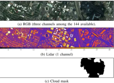
(a) RGB (three channels among the 144 available).
6 9 12 15 18 21 24 27 30
(b) Lidar (1 channel)
(c) Cloud mask
Fig. 3: The 2013 GRSS DFC dataset.
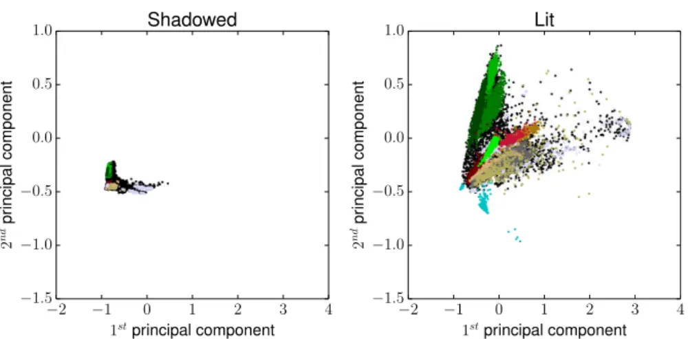
signature and its altitude on the DSM. Labels are provided for around 15000 pixels as shown in table I. The shadow of a cloud affects the right part of the image, leading to important shifts in the spectral signatures of the hyperspectral image. Figure 2 shows the lit and shadowed domains on the same scale. Thus, adaptation is required to allow a single classifier to deal correctly with both shadowed and lit areas. We obtained a cloud mask (fig. 3c) by thresholding the magnitude of the bands corresponding to RGB and Near-Infrared and using manual intervention to remove some of the spurious points. We can therefore divide our image in two domains : the source domain contains all the pixels affected by the cloud shadow while the target domain is the remainder of the image.
B. Experimental setup
The labels provided for this dataset are divided into two groups : one for training and one for testing. The training set only contains pixels that are not affected by the shadow while the testing set contains both lit and shadowed pixels.
To evaluate the performance of our adaptation procedure, we use a one-vs-one SVM with a Gaussian kernel. After model selection by cross-validation in the ranges γ= [10−3, ...,102]
and CSVM = [100, ...,103], we obtained the optimal SVM
parameters. For each pixel, the following features are used by the SVM :
• 144 spectral bands • 1 LiDAR band
• 6 bands obtained by applying opening by reconstruction
and closing by reconstruction on the LiDAR band with three different square structuring elements of sizes : {7, 19, 31}. Morphological filters are often used in remote sensing pixel classification to enforce the smoothness of the decision function in the spatial domain [19]. The spectral bands are normalized by their overall maximal value and the lidar band is normalized by its maximal value. We set the nearness threshold α = 0.2 and the farness threshold β= 0.3. We use C = 200 for the fine graphs and ex-periment with two different values for KS = KT = [50, 100].
The value of C depends on the dataset and should be set large enough to yield a good representation of data. Since the
finegraphs are used only for the computation of the geodesic distances, which are computed only once at the beginning of the process, C can be increased without impacting the performances.
We compare the proposed netCC algorithm with histogram matching applied on all the spectral bands. Since we are in-terested in the classification improvement after adaptation, we consider two separate testing scenarios : testing pixels under the shadow only and all testing pixels. In the experiments, we study the variability with regard to 2 parameters : the dimensionality of the space where the matching is performed (npc) and the number of nodes in the coarse graphs (KS, KT). For each choice of parameters, we run the whole graph matching procedure (clustering, matching) 10 times and report the average performances.
V. RESULTS AND DISCUSSIONS
With the setting described above, the proposed netCC algorithm converges in a limited number of iteration, typically around 100. This corresponds to an average running time of a few minutes on a laptop (Intel i5).
Table II shows the results when using only pixels under the shadow as test samples (around 1400 points). Without adaptation, we get a κ score of 0.131, which is very low. We can see that by using histogram matching or netCC, we respec-tively reach a performance of 0.36-0.47, which is acceptable considering that this is a problem involving 15 classes, and some of them are very similar (e.g. there are three types of grass, two types of parking lots, two types of buildings). We obtain an improvement of 0.01 to 0.11 κ points by using netCC over histogram matching. This corresponds to an increase in accuracy of about 11%. The choice of the number of centroids, KS and KT, has an important influence on the results. This
is of course dependent on the problem, but on our testing dataset, it seems KS = KT = 50 is enough to get a good
representation of the data manifold and increasing to 100 mostly increases the number of clusters near the center of the
−2 −1 0 1 2 3 4 1stprincipal component −1.5 −1.0 −0.5 0 .0 0 .5 1 .0 2 nd p ri n ci p a l co m p o n e n t Shadowed −2 −1 0 1 2 3 4 1stprincipal component −1.5 −1.0 −0.5 0 .0 0 .5 1 .0 2 nd p ri n ci p a l co m p o n e n t Lit
Fig. 2: Projection of the two domains on the two first principal components. Colors indicate class membership (black is unlabeled).
graph. This makes it harder to find a set of correspondences that satisfy all nearness potentials. On the other hand, we see that increasing the number of principal components (npc) has a positive effect on the performances. This is because with less principal components the reconstruction will be of lower quality.
Table III reports the results obtained when using of all the testing labels (about 12000 points). We get a small increase in performance when using netCC over histogram matching. The effect of DA is less visible due to the large number of test points in the lit area that do not benefit from adaptation.
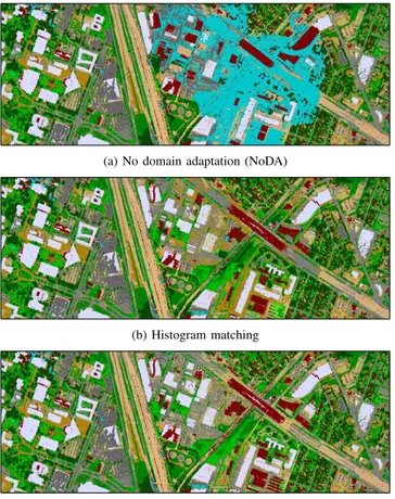
Figure 4 shows classification maps for the right part of the image with the tested methods. Visually, the benefits of domain adaptation are obvious. We can see that without domain adaptation, the classifier fails to produce a meaningful result and classifies everything as water. The problem disappears when adapting the spectra prior to classification.
Figure 5 provides a magnified view of two areas where his-togram matching and netCC result in different classifications. In the second row, we can see that histogram matching causes a grass area (visible on the labels and the flat lidar) to be clas-sified as trees while netCC correctly classify it as grass. In the third row, a zoom on an urban area is shown. From the RGB and lidar images, it is clear this area contains buildings, some of which are misclassified as grass after histogram matching. With netCC, they are correctly classified as buildings, albeit not of the correct class. The same observation can be made for some roads which are misclassified as soil after histogram matching.
VI. CONCLUSION
In this paper, we propose an extension of the correlated correspondence algorithm for graph matching to handle d dimensional datasets. We propose the use of descriptors used in network analysis to guide the matching process. To reduce the computational costs, we use a two-levels graph and only allow matches between neighbors in the descriptor space.
TABLE II: Results with the shadowed test points
Overall Accuracy (%) Kappa (κ) npc KS, KT µ σ µ σ 10 100 53.3 4.1 0.471 0.044 50 53.9 4.4 0.476 0.047 5 100 44.4 4.3 0.375 0.046 50 49.1 3.2 0.424 0.035 2 100 43.6 3.3 0.368 0.036 50 48.0 7.4 0.412 0.078 Histogram matching 42.2 0.0 0.360 0.000 No adaptation 18.6 0.0 0.131 0.000
TABLE III: Results with all the test points
Overall Accuracy (%) Kappa (κ) npc KS, KT µ σ µ σ 10 100 89.3 0.5 0.884 0.005 50 89.4 0.5 0.885 0.006 5 100 88.3 0.5 0.873 0.005 50 88.8 0.4 0.879 0.004 2 100 88.2 0.4 0.872 0.004 50 88.7 0.9 0.877 0.009 Histogram matching 88.0 0.0 0.870 0.000 No adaptation 85.2 0.0 0.841 0.000
Experiments on a challenging real-world dataset show good performances and a significant improvement over histogram matching. Future research directions could focus on the choice of descriptors and on the use of different potentials. Deeper exploration and sensitivity analysis of the various parameters would also be interesting, as well as the application to other datasets.
(a) No domain adaptation (NoDA)
(b) Histogram matching
(c) netCC
Fig. 4: Comparison of classification maps for the three meth-ods on the part of the image affected by the shadow of the cloud.
RGB LiDAR labels NoDA HM netCC
RGB LiDAR labels NoDA HM netCC
Fig. 5: Zoom on specific areas to compare the classification maps. The top row shows the RGB image with the zoomed areas highlighted : middle row corresponds to the red zoom and bottom row to the green zoom.
transport the points for a given transformation of the nodes. In our current implementation, the local transformation is a simple translation, but more generic classes of transformation (e.g. affine) could be considered and possibly improve the performance of the classifier trained in the adapted domain.
ACKNOWLEDGMENT
This work has been partially funded by the Swiss NSF (grant PZ00P2-136827) and by the Belgian Science Office (BELSPO, grant SR/00/154). We acknowledge Prof. Prasad and the IEEE IADF TC for providing the 2013 Data Fusion Contest Data.
REFERENCES
[1] J. Qui˜nonero-Candela, M. Sugiyama, A. Schwaighofer, and N. D. Lawrence, Dataset shift in machine learning, ser. Neural information processing series. Cambridge, MA: MIT Press, 2009.
[2] G. Camps-Valls, D. Tuia, L. Bruzzone, and J. Benediktsson, “Advances in hyperspectral image classification: Earth monitoring with statistical learning methods,” IEEE Signal Proc. Mag., vol. 31, no. 1, pp. 45–54, 2014.
[3] D. Lunga, S. Prasad, M. Crawford, and O. Ersoy, “Manifold-learning-based feature extraction for classification of hyperspectral data,” Signal
Proc. Mag., vol. 31, no. 1, pp. 55–67, 2014.
[4] H. Bunke, “Error correcting graph matching: on the influence of the underlying cost function.” IEEE Trans. Pattern Anal. Mach. Intell., vol. 21, pp. 917–922, 1999.
[5] D. Tuia, J. Mu˜noz-Mari, L. Gomez-Chova, and J. Malo, “Graph match-ing for adaptation in remote sensmatch-ing,” IEEE Trans. Geosci. Remote Sens., vol. 51, pp. 329–341, 2013.
[6] C. Wang, P. Krafft, and S. Mahadevan, “Manifold alignment,” in
Manifold Learning: Theory and Applications, Y. Ma and Y. Fu, Eds.
CRC Press, 2011.
[7] C. Wang and S. Mahadevan, “Heterogeneous domain adaptation using manifold alignment,” in International Joint Conference on Artificial
Intelligence (IJCAI), Barcelona, Spain, 2011.
[8] ——, “Manifold alignment without correspondence,” in International
Joint Conference on Artificial Intelligence, Pasadena, CA, 2009.
[9] D. Tuia, M. Volpi, M. Trolliet, and G. Camps-Valls, “Semisupervised manifold alignment of multimodal remote sensing images,” IEEE Trans.
Geosci. Remote Sens., in press.
[10] R. Szeliski, R. Zabih, D. Scharstein, O. Veksler, V. Kolmogorov, A. Agarwala, M. Tappen, and C. Rother, “A comparative study of energy minimization methods for Markov Random Fields,” in Proc. ECCV, 2006.
[11] G. Moser, S. B. Serpico, and J. A. Benediktsson, “Land-cover mapping by Markov modeling of spatial-contextual information,” Proceedings of
the IEEE, vol. 101, pp. 631–651, 2013.
[12] J.-P. Jacobs, G. Thoonen, D. Tuia, G. Camps-Valls, B. Haest, and P. Scheunders, “Domain adaptation with hidden Markov Random Fields,” in Proc. IGARSS, 2013.
[13] D. Anguelov, P. Srinivasan, H.-C. Pang, D. Koller, S. Thrun, and J. Davis, “The correlated correspondence algorithm for unsupervised registration of nonrigid surfaces,” 2005.
[14] P. Crucitti, V. Latora, and S. Porta, “Centrality measures in spatial networks of urban streets,” Phys. Rev. E, vol. 73, p. 036125, 2006. [15] V. Kolmogorov, “Convergent tree-reweighted message passing for
en-ergy minimization,” IEEE Trans. Pattern Anal. Mach. Intell., vol. 28, pp. 1568–1583, 2006.
[16] J. Pearl, Probabilistic reasoning in intelligent systems: networks of
plausible inference. Morgan Kaufmann, 1988.
[17] M. Bernstein, V. De Silva, J. C. Langford, and J. B. Tenenbaum, “Graph approximations to geodesics on embedded manifolds,” Stanford University, Tech. Rep., 2000.
[18] F. Pacifici, Q. Du, and S. Prasad, “Report on the 2013 IEEE GRSS data fusion contest: Fusion of hyperspectral and LiDAR data,” IEEE Remote
Sens. Mag., vol. 1, pp. 36–38, 2013.
[19] M. Fauvel, Y. Tarabalka, J. Benediktsson, J. Chanussot, and J. Tilton, “Advances in spectral-spatial classification of hyperspectral images,”