HAL Id: hal-01308019
https://hal.archives-ouvertes.fr/hal-01308019
Submitted on 27 Apr 2016
HAL is a multi-disciplinary open access
archive for the deposit and dissemination of
sci-entific research documents, whether they are
pub-lished or not. The documents may come from
teaching and research institutions in France or
abroad, or from public or private research centers.
L’archive ouverte pluridisciplinaire HAL, est
destinée au dépôt et à la diffusion de documents
scientifiques de niveau recherche, publiés ou non,
émanant des établissements d’enseignement et de
recherche français ou étrangers, des laboratoires
publics ou privés.
Sound event detection in remote health care - Small
learning datasets and over constrained Gaussian
Mixture Models
Jugurta Montalvão, Dan Istrate, Jérôme Boudy, Joan Mouba
To cite this version:
Jugurta Montalvão, Dan Istrate, Jérôme Boudy, Joan Mouba. Sound event detection in remote health
care - Small learning datasets and over constrained Gaussian Mixture Models. EMBC 2010 : 32nd
Annual International Conference of the IEEE Engineering in Medicine and Biology Society, Aug 2010,
Buenos Aires, Argentina. pp.1146-1149, �10.1109/IEMBS.2010.5627149�. �hal-01308019�
Sound Event Detection in Remote Health Care – Small Learning
Datasets and Over Constrained Gaussian Mixture Models
Jugurta Montalv˜
ao, Dan Istrate, Joan Mouba and Jerˆome Boudy
Abstract— The use of Gaussian Mixture Models (GMM), adapted through the Expectation Minimiza-tion (EM) algorithm, is not rare in Audio Analy-sis for Surveillance Applications and Environmental sound recognition. Their use, at a first glance, is founded on the good qualities of GMM models when aimed at approximating Probability Density Func-tions (PDF) of random variables. But in some cases, where models are to be adapted from small sample sets of specific and locally recorded signals, instead of large but generic databases, a problem of balance between model complexity and sample size may play an important role. From this perspective, we show, through simple sound classification experiments, that constrained GMM, with fewer degrees of freedom, as compared to GMM with full covariance matrices, provide better classification performances. Moreover, pushing this argument even further, we also show that a Parzen model (seen here as an over-constrained GMM) can do even better than usual GMM, in terms of classification error ratio.
I. INTRODUCTION
Acoustic Event Detection and Classification is a recent sub-area of computational auditory scene analysis [1] where particular attention has been paid to automatic surveillance systems [2], [3], [4]. More specifically, the use of audio sensors in surveillance and monitoring ap-plications has proven to be particularly useful for the detection of distress situation events, mainly when the person suffers from cognitive illness. The recent research work in medicine has concluded that some persons with mild cognitive impairment will develop Alzheimer in the future. The efficient detection and recognition of the distress situation is one part of the socially assistive robotics technology [5] aimed at providing affordable personalized cognitive assistance.
In recent works, it has been shown that automatic detection of relevant events for remote healthcare can be done in a rather conventional way, through the anal-ysis of short segments (less than 50 ms, typically) of digitalized signals from microphones strategically placed into rooms where the subject to be monitored lives (e.g. places in the house of a elderly person under medical
J. Montalv˜ao is with Faculty of Electrical Engineering, Univer-sity of Sergipe, S˜ao Crist´ov˜ao, CEP. 49100-000, Brasil jmontal-vao@ufs.br
D. Istrate and J. Mouba are with the ESIGETEL school, responsible of ANASON Team, 1, Rue du Port de Valvins, 77210 Fontainebleau-Avon, Francedan.istrate@esigetel.fr, joan.mouba@esigetel.fr
J. Boudy is with the T´el´ecom SudParis, 9 Rue Charles Fourier, 91011, Evry, FranceJerome.Boudy@it-sudparis.eu
care). These short segments of sounds are then processed and features are extracted, much like what is done in speech or speaker recognition. Indeed, features such as Mel Frequency Cepstral Coefficients (MFCC) [6] and Matching Pursuit (MP) [7], along with Gaussian Mixture Models (GMM), are not rarely deployed for this kind of task.
Signals to be detected in healthcare scenarios show high variability from one instance to another, even for supposedly equivalent acoustic sources (intra-class vari-ability). For instance, one can easily notice, through simple experiments, that door clapping sounds strongly depend on the door size, on the material the door is made of, and even on the room acoustics. This high variability explains indeed why recognition rates rapidly fall with increasing number of classes, as discussed in [7], and it rises a relevant question concerning adaptation of general classifiers to specific scenarios. More precisely, once a classifier was trained to recognize some classes of relevant sounds, one straightforward approach to adapt this classifier to a specific environment (e.g. a given apartment or house) is the adjustment of the universal class models to the specificities of the new environment, through some few new sound recordings locally acquired. But for very irregular classes of sounds, where new instances (new recordings) may strongly deviate from previously learnt universal model, this adaptation may be equivalent to obtaining a new model, instead of an incremental adaptation. In such cases, usual probabilistic models based on Gaussian mixtures (i.e. GMM), whose mixture parameters are found through the well-known Expectation-Maximization (EM) algorithm [8], demand a certain amount of new training signals to properly work. The acquisition of new training samples in loco, for model adjustment, may become cumbersome, even if this number is just, for instance, 10 new recordings per class. It is noteworthy that, in the literature, models are usually trained with much more than 10 recordings per class.
By contrast, if a classifier is able enough to properly learn a model from a few samples (recordings) per class, then the need for a universal model may be dropped in favor of full model learning in loco, from few recordings made in each new environment.
Probabilistic models are typically based on Probability Density Function (PDF) estimation from limited data sets, which is a classical problem in pattern recognition [9]. From this perspective, in this work, we focus on
the problem of how to obtain useful GMM based PDF approximations, even when datasets are too small.
Our approach is greatly simplified if we define model regularization in a wide point of view, from which Parzen models with Gaussian kernels are regarded as over-regularized GMM, as explained in Section II. Signal segmentation is explained in Section III whereas, in Section IV, we gather experimental evidences that the tradeoff between model degree of freedom and amount of data for model adaptation may be a key for useful probabilistic classifier, even with very small datasets. Finalli, in Section V, we briefly analyze our claims as a contribution to improve remote healthcare applications.
II. PDF ESTIMATION AND MODEL REGULARIZATION
PDF estimation from limited data sets is a classical problem in pattern recognition for which many approxi-mated solutions are presented in literature [9], [11]. Prob-ably the most widely used PDF model is GMM, along with EM algorithm for parameter adaptation (learn-ing). It is worth noting that, though the EM is not the fastest algorithm for GMM optimization [10], it is usually simpler to apply, which can partially explain its widespread popularity in many application fields. However, in addition to its possibly poor convergence rate (depending on the data distribution and the initial estimates of its parameters), it also presents the following drawbacks [11]:
(a) Its likelihood-based criterion presents a multitude of useless global maxima;
(b) Convergence to parameter values associated with singularities is more likely to occur with small data sets, and when centers are not well separated. Indeed, it is well-known that likelihood is often unrepresentative in high dimensional problems, which can be true in some low-dimensional problems as well [12]. In order to cope with these drawbacks, model regularization is the usual solution, through which, the searching throughout the parameter space is constrained.
Therefore, as far as regularization approaches lead to parametric constraints, we propose a wide point of view from which any reduction imposed to the mixture freedom degree is regarded as a kind of model regu-larization. Accordingly, regularization strategies can be roughly split into four categories, namely:
(I) The most usual approach to regularization is based on the addition of a term to the unconstrained criterion function, which expresses constraints or desirable prop-erties of solutions.
(II) For models obtained via clustering-like algorithms (including the EM, which can be loosely seen as a soft clustering algorithm [11]), a straightforward regu-larization approach is that of averaging estimates from many independent initializations. In [13], for instance, two approaches to GMM regularization are compared: one based on averaging (category II), and the other
based on an explicit regularization term (category I). Both provided improved models (if compared to the unconstrained one), with similar performances.
(III) For Mixture Models, regularization can be easily obtained by imposing constraints on the mixture compo-nent parameters (e.g. by imposing constraints or lower bounds on the covariance matrix of Gaussian kernels in GMM).
(IV) Conexionist models (e.g. artificial neural net-works) can also be regularized, or partially regularized by pruning [14], though it is not always explicitly referred to as a regularization procedure. This includes Radial Basis Functions Neural Networks, which are structurally related to GMM.
Thanks to this wide regularization concept, the non-parametric Parzen method [9], [11] can loosely be re-garded as a mixture model based method with strongly-constrained mixture components (category III). Thanks to this strong constraint on the Gaussian placement, the Parzen approach gives an instantaneous PDF approxi-mation (no iterations) but, in spite of its simplicity, it is known that, under some constraints on the Parzen window width parameter, the convergence of the esti-mated PDF with the actual one is guaranteed, when the number of samples tends to infinity [11]. In other words, many small isotropic (radial basis) Gaussian kernels, with identical dispersion, can virtually approximate any PDF “shape”. This corresponds to a trade from kernel complexity (elliptical kernels, for instance, typically ob-tained via the EM approach) to kernel number.
Although EM and Parzen approaches come from differ-ent paradigms – namely, parametric and nonparametric PDF estimation, respectively – they share a striking structural similarity, whenever the Parzen method is based on Gaussian kernels. In both cases, the actual PDF is approximated by a Mixture of Gaussians. How-ever, Gaussian Mixture Models provided by the Parzen method are intrinsically regularized, for kernel centers cannot move (structural regularization - category IV) and identical radial dispersions are imposed on all kernels (parametric regularization - category III). In this paper, we propose a useful point of view from which both kinds of PDF estimates – i.e. GMM learnt via EM and Parzen – are seen as Gaussian Mixture Models (GMM), with different levels of regularization. More precisely, starting from GMM with unconstrained covariance matrices (full covariance matrices), we can obtain several levels of parametric regularization, through the replacement of full covariance (Level 0) matrices with:
• Level 1: one diagonal covariance matrix for each Gaussian in the Mixture;
• Level 2: one scalar covariance matrix for each Gaus-sian in the Mixture;
• Level 3: the same scalar covariance matrix for all Gaussian in the Mixture; On this third level of parametric model regularization (category III), we impose identical and isotropic Gaussian kernels
throughout the mixture. Structurally, we are very close to the Parzen model with Gaussian kernels. In fact, the only remaining difference is that Gaussian centers cannot move during adaptation/learning of the Parzen model. Therefore, Parzen models can be seen as the result of a fourth level of GMM regularization, namely:
• Level 4: similar to Level 3, but Gaussian centers are not allowed to move during model adapta-tion/learning (i.e. the Parzen model).
III. SIGNAL SEGMENTATION AND SHORT-TIME ANALYSIS
Raw signals are represented by samples, s(n) ∈ ℜ, where n ∈ ℵ. In this work, samples are regularly taken at 16KHz. We assume that each raw signal, corresponding to each recorded file in our database (see Section IV), contains, at least, one relevant event corresponding to one of those sound sources (arbitrarily limited here to 6): 1) Glass Breaking 2) Screaming 3) Door Clapping 4) Step Sound 5) Cough
6) Metal object fall
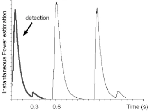
Therefore, we first use an algorithm to detect a single event and crop the corresponding subset of samples, ss(k), where k ∈ {kbegin, ..., kend}. This segmentation task is done here by a very simple algorithm, based on power measurement, which can be summarized as follows:
1) s(n) ← s(n)/σs (σs stands for the estimated stan-dard deviation of s(n))
2) p(n) ← s(n)2
(noisy instantaneous power estima-tion)
3) pf(1) ← 2 (pf stands for the lowpass-filtered power estimation) 4) for k = 2 to N if (p(k) > pf(k − 1)) pf(k) ← 0.005p(k) + 0.995pf(k − 1) else pf(k) ← 0.001p(k) + 0.999pf(k − 1) end end
5) kbegin takes the value of k for which pf(k) first crosses level 2.1 (2.0 is the expected steady level for white noise).
6) kend takes the value of k for which pf(k) crosses min(pf) + 0.1.
In other words, this algorithm just filters the noisy in-stantaneous power estimation with a nonlinear low-pass IIR filter, which is more reactive to power increments (in order to detect fast attacks of our target noises). Thus, it uses two level-crossing detectors to segment the signal to be analyzed. Figure 1 illustrates this segmentation procedure for a signal containing three step sounds (class
4). It is worth noting that only the first step sound is segmented.
Fig. 1. Signal segmentation through power contour – note that only the first relevant part of the signal is taken.
In spite of its simplicity, this algorithm is able to satisfactorily segment targeted sounds even at very low Signal to Noise Ratio (SNR), if noise has an almost stationary power through time.
Afterwards, segmented intervals of sound, ss(k), for each sound file in the database, are short-time analyzed. That is to say that windows of 500 consecutive samples (approx. 31 ms at 16KHz) are taken as signal vectors to be projected in a new space of reduced dimension. For MFCC based analysis, each 500-dimensional vector is mapped into a 24-dimensional space, each dimension corresponding to one Mel-Cepstral Coefficient.
IV. EXPERIMENTAL RESULTS
In this Section, we present experimental results ob-tained with a subsets of the sound database gathered in the framework of the (European) CompanionAble Project (http://www.companionable.net/ ), by D. Is-trate and fellows. This subset contains:
• Class 1: 574 files with door clapping sounds • Class 2: 88 files with glass breaking sounds • Class 3: 22 files with step sounds
• Class 4: 73 files with screaming sounds (males and females)
• Class 5: 41 files with cough sounds
• Class 6: 12 files with sounds of metal object falls All files in this subset were recorded at a sampling rate of 16KHz, and only a single channel (monaural sound) of each record is used in this work.
Only five files, from each class, are arbitrarily chosen to represent the classes (training samples). They are then processed (MFCC projection of short-time over-lapping windows), and obtained 24-D vectors of coeffi-cients, x, are seen as instances of 6 multivariate ran-dom variables, X1, . . . , X6, corresponding to 6 classes of sound. Moreover, we use these instances to estimate the underlying PDF associated to each random variable, fX1(x), . . . , fX6(x).
As for the PDF estimation, all models are given by: fXi(x) = M X i=1 αig(x|ci, Ri) (1) where Θ = [α1, . . . , αM, c1, . . . , cM, R1, . . . , RM] stands for the mixture parameter vector, and g(x|ci, Ri) corre-sponds to the i-th Gaussian kernel of the mixture, with mean vector and covariance matrix given by ci and Ri, respectively. We further impose that 0 ≤ αi ≤ 1 and PM
i=1αi= 1.
This parametric model includes the Parzen model with Gaussian kernels, whenever the following restrictions on the parameter vector are imposed:
Θ= [αi= 1/M, ci = xi, Ri= σ2I] (2) where i = 1, . . . , M .
These restrictions lead to a Gaussian Mixture Model equivalent to that obtained by the nonparametric Parzen method, where each Gaussian kernel center, ci, is directly given by a sample vector. Applying these restrictions to Equation 1 yields: fXi(x) = (1/M ) M X i=1 g(x|xi, σ2 I) (3) Consequently, as we can observe in Equation 2, under such strong constraints, the only free parameter of the model is σ, the Gaussian radial dispersion.
This is a single scalar parameter, and optimizing Θ through likelihood maximization, in this case, is equiv-alent to find the value of σ that maximizes likelihood, which can be easily done by simple exhaustive one-dimensional (1D) search, through cross-validation ap-proach [11]. By contrast, free parameters in Equation 1, corresponding to conventional GMM, are adapted through EM.
In both cases – with conventional GMM or Parzen models –, any new sound is classified by comparing the averaged likelihood of each model for a given set of patterns (extracted from a recorded sound). More precisely, as far as we do not accept a no-classification result (reject class), we just pick-up the class associated to the highest averaged likelihood as a pointer to the class from which the analyzed sound is more likely to come from.
Five experiments were carried out, from unconstrained GMM (Level 0 - see Section II for further details) to over-constrained GMM (Level 4 - Parzen models). These experiments were designed to highlight the impact of constraint/regularization, in an increasing way, of GMM on performance assessment. Concerning GMM structure, the number of Gaussians is fixed at 8 (empirically opti-mized from available data). Another important imple-mentation aspect is that Gaussian centers, in EM algo-rithm, are initialized with points taken at random from the training set. Consequently, we keep initialization of both GMM and Parzen models as similar as possible. It
TABLE I
Averaged Classification Error Ratio, model training with 5 randomly chosen files, and tested with other 7 files
Mixture Model av. error ratio (%) 95% conf. interval
GMM, full 77.4% ±2.3% GMM, diag. 66.7% ±1.0% GMM, scalar 34.3% ±8.7% GMM, single scalar 32.8% ±9.0% Parzen models 16.7% ±6.1% TABLE II
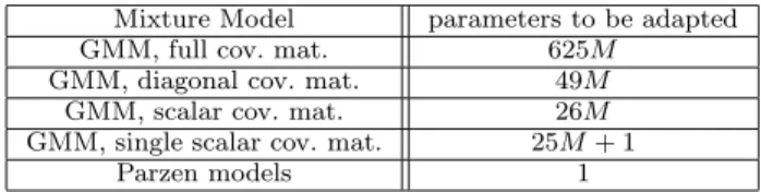
Number of free parameters per model, in 24-D parameter space
Mixture Model parameters to be adapted
GMM, full cov. mat. 625M
GMM, diagonal cov. mat. 49M
GMM, scalar cov. mat. 26M
GMM, single scalar cov. mat. 25M + 1
Parzen models 1
contrasts with a rather popular approach where K-means algorithm is used to initialize EM.
Table I presents our results, in terms of error ratios, for Gaussian mixtures under four levels of regularization 1
, including the Parzen model as an over-regularized mixture.
It is clear that increased regularization improves clas-sification performance, and we believe that the huge amount of free parameters in usual GMM (i.e. with full or diagonal covariance matrices), as compared to the limited amount of data for model training, mainly explains the performance gain of more constrained (wide-sense regularized) models. To further highlight the decreasing degree of freedom in each model, we explicitly present their respective number of parameters to be adapted, per level of parametric and structural regularization. All models lay in a 24-D space, and M stands for the number of Gaussian kernels:
V. CONCLUSIONS
In this preliminary work, we present evidences that traditional GMM adapted with EM algorithms may not be a suitable PDF model to be rained with a small amount (recorded sounds) of training samples. Though it was presented through experiments with a reduced number of classes, we may easily recognize that it comes from a wider and quite older discussion concerning PDF estimation in pattern recognition domain, not always taken into account in practical applications. Here, we compared Gaussian Mixture Models with 5 levels of parametric and structural wide-sense regularization (as proposed in Section II), from GMM with full covariance matrices to Parzen model with Gaussian kernels (seen
here as an over-constrained GMM). By comparing per-formances with these models, we gave one illustration, through simple experiments, that even if both GMM and Parzen models are theoretically able to converge to the true PDF to be estimated, under training data ”shortage”, they provide remarkably different error ratios. What we observe through our experiments is that, with a reduced number of instances for the model training, the path taken by the Parzen model seems to be more performing, in terms of classification.
Thus, what we claim here is that it is a clear matter of model regularization: the more regularized, the better, if the number of training patterns are too limited, and we highlight that training data “shortage” is indeed a fre-quent condition met in healthcare applications, since one needs to train specific sound models for each new envi-ronment to be monitored (e.g. care receiver’s house, flat). Moreover, combined to incremental training strategies, this approach can offer a good and fast existing sound models adaptation for a given environment presenting some time variabilities.
VI. ACKNOWLEDGMENTS
The authors gratefully acknowledge the financial sup-port of the Brazilian Conselho Nacional de Desen-volvimento Cient´ıfico e Tecnol´ogico (CNPq), as well as the contribution of the European Community’s Seventh Framework Programme (FP7/2007-2011), Companion-Able Project (grant agreement n. 216487).
References
[1] G. Valenzise, L. Gerosa, M. Tagliasacchi, F. Antonacci, A. Sarti, “Advanced Video and Signal Based Surveillance”, in AVSS 2007, vol. 2, issue 5-7, 2007, pp 21-26.
[2] D. Wang, G. Brown, Computational Auditory Scene Analysis: Principles, Algorithms and Application, Wiley-IEEE Press, 2006.
[3] C. Zieger, M. Omologo, “Acoustic event classification using a distributed microphone network with a GMM/SVM combined algorithm”, in Interspeech, September 2008, pp 115-118. [4] D. Feil-Seifer, M.J. Mataric, “Defining socially assistive
robotics”, in Proc. IEEE International Conference on Reha-bilitation Robotics (ICORR’05), Chicago, Il, USA, June 2005, pp 465-468.
[5] J.L. Rouas, J. Louradour, S. Ambellouis, “Audio Events De-tection in Public Transport Vehicle”, in Proc. of the 9th International, IEEEConference on Intelligent Transportation System, Sept. 2006, pp 733-738.
[6] D. Istrate, M. Binet, S. Cheng
”“Real time sound analysis for medical remote monitoring”, in Proc. IEEE EMBC, Vancou-ver, Canada, Aug. 2008, pp 4640-4643.
[7] S. Chu, S. Narayanan, C.-C. J. Kuo, Environmental sound recognition with time-frequency audio features, Trans. Audio, Speech and Lang. Proc., vol. 17, no 6, 2009, pp 1142-1158. [8] A. Dempster, N. Laird, D. Rubin, Maximum likelihood
esti-mation from incomplete data using the em algorithm, J Royal Stat Soc., vol. 39, 1977, pp 1-38.
[9] R. O. Duda, P. E. Hart, and D. G. Stork, Pattern Classifica-tion, John Wiley & Sons, Inc., 2nd ediClassifica-tion, 2001.
[10] D. M. Titterington, A. F. M. Smith, U. E. Makov, Maximum likelihood estimation from incomplete data using the EM algo-rithm, John Wiley & Sons, Inc., 1985.
[11] A. Webb, Statistical Pattern Recognition, Wiley, 2nd edition, 2002.
[12] D. J. C. MacKay, Information Theory, Inference, and Learn-ing Algorithms, Cambridge University Press, 2003.
[13] D. Ormoneit and V. Tresp. Improved gaussian mixture density estimates using bayesian penalty terms and network averaging, The MIT Press, Advances in Neural Information Processing Systems, 1996, pp 542-548.
[14] S. Haykin, Neural Networks, A Comprehensive Foundation, Prentice-Hall, Englewood Cliffs, USA, 2 edition edition, 1999.