Hybrid Risk Assessment Model Based on Bayesian Networks

HAL Id: hal-01393744

https://hal.archives-ouvertes.fr/hal-01393744

Submitted on 8 Nov 2016

HAL is a multi-disciplinary open access

archive for the deposit and dissemination of

sci-entific research documents, whether they are

pub-lished or not. The documents may come from

teaching and research institutions in France or

abroad, or from public or private research centers.

L’archive ouverte pluridisciplinaire HAL, est

destinée au dépôt et à la diffusion de documents

scientifiques de niveau recherche, publiés ou non,

émanant des établissements d’enseignement et de

recherche français ou étrangers, des laboratoires

publics ou privés.

Hybrid Risk Assessment Model Based on Bayesian

Networks

François-Xavier Aguessy, Olivier Bettan, Gregory Blanc, Vania Conan, Hervé

Debar

To cite this version:

François-Xavier Aguessy, Olivier Bettan, Gregory Blanc, Vania Conan, Hervé Debar. Hybrid Risk

Assessment Model Based on Bayesian Networks. 11th International Workshop on Security, IWSEC

2016, Sep 2016, Tokyo, Japan. pp.21 - 40, �10.1007/978-3-319-44524-3_2�. �hal-01393744�

Hybrid Risk Assessment Model based on

Bayesian Networks

Fran¸cois-Xavier Aguessy1,2_{, Olivier Bettan}1_{, Gregory Blanc}2_{, Vania Conan}1_, and Herv´e Debar2

francois-xavier.aguessy@telecom-sudparis.eu

1 _{Thales, 4 avenue des Louvresses, 92622 Gennevilliers, France} 2

SAMOVAR, T´el´ecom SudParis, Universit´e Paris Saclay, 9 rue Charles Fourier, 91011 Evry, France

Abstract. Because of the threat posed by advanced multi-step attacks, it is difficult for security operators to fully cover all vulnerabilities when deploying countermeasures. Deploying sensors to monitor attacks ex-ploiting residual vulnerabilities is not sufficient and new tools are needed to assess the risk associated with the security events produced by these sensors. Although attack graphs were proposed to represent known multi-step attacks occurring in an information system, they are not directly suited for dynamic risk assessment. In this paper, we present the Hybrid Risk Assessment Model (HRAM), a Bayesian network-based extension to topological attack graphs, capable of handling topological cycles, making it fit for any information system. This hybrid model is subdivided in two complementary models: (1) Dynamic Risk Correlation Models, correlat-ing a chain of alerts with the knowledge on the system to analyse ongocorrelat-ing attacks and provide the hosts’ compromise probabilities, and (2) Future Risk Assessment Models, taking into account existing vulnerabilities and current attack status to assess the most likely future attacks. We vali-date the performance and accuracy of this model on simulated network topologies and against diverse attack scenarios of realistic size.

1

Introduction

Information systems concentrate invaluable information resources, generally com-posed of the computers and servers that process the data of an organisation. Given the number and complexity of attacks, security teams need to focus their actions on the most important attacks, in order to select the most appropriate security controls [20]. Importance in our context is related to the risk the attack induces on the missions of the information system. The most impacting attacks are multi-step attacks. A multi-step attack is a complex attack composed of sev-eral successive steps. Each step may be illegitimate (e.g., the exploitation of a vulnerability in software) or legitimate (e.g., a user with administrators privilege accessing sensitive data). For example, an attacker first subverts a client com-puter using a spear-phishing email exploiting a vulnerability, then attacks the Active Directory to get administrator privileges, and, thanks to this privilege, accesses a database server that contains sensitive data.

In order to defend against complex attacks, we need to model them and assess associated risks. But risk assessment, and in particular dynamic risk as-sessment (i.e., regular update of risk asas-sessment in operational time, according to the occurring attacks) is not easy. Several models have been proposed in the literature to formalise multi-step attacks, mainly tree or graph-based models. An attack graph, for example, is a risk analysis model grouping all the paths an attacker may follow in an information system. Several tools to generate attack graphs exist. Their use is attractive because they leverage already available in-formation (vulnerability scans and network topology). However, attack graphs are static and do not contain detections or attack status and thus are not fitted for dynamic risk assessment. Several extensions of static risk assessment models have been proposed in the literature to accommodate dynamic risk assessment, but they suffer from common limitations, such as existing cycles.

According to the National Information Assurance Glossary [18], a risk is “a measure of the extent to which an entity is threatened by a potential circum-stance or event, and typically a function of 1) the adverse impacts that would arise if the circumstance or event occurs; and 2) the likelihood of occurrence”. As a result, the risk is generally considered in Information Security Management Systems (ISMS) as the combination of the likelihood of the exploitation of vul-nerabilities and their impact on the system. Determining the risk in a system is the result of a 5-step process detailed by the National Institute of Standards and Technology (NIST) in [19], as shown in Figure 1. In this process, the step (2.c) is the determination of the likelihood of occurrence of the attacks. It takes as input the potential threat sources and the vulnerabilities and attack predispos-ing conditions. Once the likelihood of attacks has been assessed, the next step is to determine their magnitude of impact. Finally, from likelihood and impact, we can compute the risk. In order to make risk assessment dynamic, the process is maintained over time and its results have to be communicated regularly to security management operators.

Fig. 1. Risk Assessment Process [19]

Step 1 : Prepare for Assessment

Step 2 : Conduct Assessment 2.a) Identify Threat Sources and Events 2.b) Identify Vulnerabilities and predisposing conditions

2.c) Determine Likelihood of Occurrence 2.d) Determine Magnitude of impact

2.e) Determine Risk S

te p 4  : M a in ta in A ss e ss m e n t S te p 3  : C o m m u n ic a te R e su lts

At an organisational level, several methods help to analyse the risk of infor-mation systems and keep those systems secure. For example, ISO/IEC 27000 [10] is the ISMS Family of Standards providing recommendations on security, risk and control in an information system. In particular, ISO/IEC 27005 [9] describes a methodology to manage the risks and implement an ISMS. Another well-known method for the analysis of risks in information systems is EBIOS (Expression of Needs and Identification of Security Objectives) [5]. These standards present global methodologies to manage risks in organisations. They generally combine (1) technical tools (e.g., vulnerability scanner) to assess, for example, the vul-nerabilities and the likelihood of attacks and (2) organisational methodologies (e.g., stakeholder interviews) to identify the critical assets and consequences of successful attacks.

The technical tools for dynamic risk assessment usually do not include a model to detect the occurring multi-step attacks and assess their likely futures. In this paper, we build such a model that aims at assessing the risk brought by the exploitation of technical vulnerabilities in a system. This model mostly focuses on the step (2.c) of the NIST’s risk assessment process of Figure 1: the determination of the likelihood of occurrence of attacks. Indeed, methodologies to estimate attacks likelihood do not depend on the system in which they are implemented, contrary to the impact assessment which may require adaptation for the target organisation. Thus, in our experimentations, we evaluate our risk model only by its likelihood results, by assuming that all compromised assets induce the same impact.

The model we propose in this paper is a new hybrid model combining attack graphs and Bayesian networks for dynamic risk assessment (DRA). This model is subdivided into two complementary models: (1) The Dynamic Risk Correlation Models (DRCMs) correlate a chain of alerts with the knowledge on the system to analyse ongoing attacks and provide the probabilities of hosts being com-promised, (2) The Future Risk Assessment Models (FRAMs) take into account existing vulnerabilities and the current attack status to assess which potential attacks are most likely to occur. DRCMs aim at threat likelihood assessment, identifying where the attack comes from. It outputs probabilities that attacks are completed and that assets of the information system are compromised. These probabilities provide security operators with the capability to manage priorities according to the likelihood of ongoing attacks. FRAMs aim at threat mitiga-tion, identifying the most likely and impacting next steps for the attacker. With respect to the current state of the art, our contributions are twofold. First, we provide an explicit model for DRA and a process for handling cycles. Second, our model provides a significant performance improvement in terms of number of nodes and vulnerabilities over the existing state of the art, enabling scalability. While classic Bayesian attack graph models are usually demonstrated over a few nodes, we show that our model can be realistically computed at the scale of an enterprise information system.

This paper is organised as follows: Section 2 presents the state of the art of the multi-step attack models. Section 3 presents topological attack graphs and

expose the problem of cycles. Then, it presents the architecture of the Hybrid Risk Assessment Model, composed of DRCMs and FRAMs. Section 4 validates the design of the hybrid model on simulated topologies. Section 5 compares our work with the related work, before concluding and presenting our future work, in Section 6.

2

State of the art

Initially proposed for risk analysis, attack graphs have been extended as Bayesian attack graphs, to include ongoing attacks probability information, which is re-quired for dynamic risk assessment.

2.1 Attack graphs

An attack graph is a model regrouping all the paths an attacker may follow in an information system. It has been first introduced by Phillips and Swiler in [24]. A study of the state of the art about attack graphs compiled from early liter-ature on the subject has been carried out by Lippmann and Ingols [16], while a more recent one was made available by Kordy et al. [14]. Topological attack graphs are based on directed graphs. Their nodes are topological assets (hosts, IP addresses, etc.) and their edges represent possible attack steps between such nodes [11]. Attack graphs are generated with attack graph engines. There are three main attack graph engines: (1) MulVAL, the Multi-host, Multi-stage Vul-nerability Analysis Language tool created by Ou et al. [21], (2) the Topological Vulnerability Analysis tool (TVA) presented by Jajodia et al. in [11,12] (com-mercialised under the name Cauldron) and (3) Artz’s NetSPA [2].

Attack graphs are attractive because they leverage readily available informa-tion (vulnerability scans and network topology). However, they are not adapted for ongoing attacks, because they cannot represent the progression of an attacker nor be triggered by alerts. Thus, they must be enriched to provide the function-alities needed to perform dynamic risk assessment, for example using Bayesian networks.

2.2 Bayesian attack graphs

A Bayesian network is a probabilistic graphical model introduced by Judea Pearl [22]. It is based on a Directed Acyclic Graph, where nodes represent random variables, and edges represent probabilistic dependencies between vari-ables [3]. For discrete random varivari-ables, these dependencies can be specified using a Conditional Probability Table associated with each child node. Bayesian networks are particularly interesting for computing inference, i.e. calculating the probability of each state of all nodes of the network, given evidences, i.e. nodes that have been set to a specific state. In the general case, exact inference is a NP-hard problem and can be done efficiently only on small networks, using the algorithm of Lauritzen and Spiegelhalter [15]. However, if the structure of

the graph is a polytree, it can be done in quasi-linear time, using Pearl’s Belief Propagation Algorithm [23].

A Bayesian attack graph, introduced by Liu and Man in [17] is an extension of an attack graph based on a Bayesian network, constituted of nodes representing a host in a specific system state (a true state means that the host is compromised) and edges representing possible exploits that can be instantiated from a source host to a target host. The major concern of building such a Bayesian network from an attack graph is due to the structure of a Bayesian network that must be acyclic, while attack graphs almost always contain cycles. To avoid cycles, Liu and Man assume that an attacker will never backtrack once reaching a compro-mised state, but do not detail how such assumption is used to build the model. In [7], Frigault and Wang use Bayesian inference in Bayesian Attack Graphs to calculate security metrics in an information system. Xie et al. present in [27] a Bayesian network used to model the uncertainty of occurring attacks. The Bayesian attack graph is enhanced with three new properties: separation of the types of uncertainty, automatic computation of its parameters and insensitivity to perturbations in the parameters choice. This model also adds nodes dedicated to dynamic security modelling: an attack action node models whether or not an action of the attacker has been performed, a local observation node models inac-curate observations (IDS alerts, logs, etc.). In [4], Cole uses a Credal network (a Bayesian network with imprecise probabilities) to represent parameters uncer-tainty and detect attack paths. He demonstrates that the unceruncer-tainty is too high for single-step attacks, but for multi-step attacks, it is possible to achieve high confidence in the detections. However, the computational costs of inferences in a Credal network are prohibitive to use it with real network topologies.

Bayesian networks add to the advantages of direct acyclic graphs powerful tools to compute and propagate probabilities between nodes of the graph. More-over, the dependencies between nodes are not AND or OR relations anymore, but are probabilities of occurrence with a set of predecessors, which is much more expressive. It is thus a very interesting model for dynamic risk assessment. However, two important problems arise when we want to use Bayesian networks for modelling ongoing multi-step attacks: (1) performance, as the inference in a Bayesian network can be very complex, and (2) a Bayesian network must be based on an acyclic graph, which is generally not the case of attack graphs. Heuristics allow to suppress cycles, but they also suppress paths that could be followed by an attacker.

3

Hybrid Risk Assessment Model

Given the advantages brought by Bayesian Attack Graphs (expressiveness, dy-namicity, powerful probability propagation tools), they provide a strong founda-tion for dynamic security modelling. Our proposal extends Bayesian Networks to be used for DRA with real-scale information systems.

3.1 Topological Attack Graph

We will first present the main input from which we build the HRAM: a topologi-cal attack graph. A topologitopologi-cal attack graph (TAG) is a directed graph consisting of topological assets, the nodes representing the assets of an information system (e.g., an IP address or a computer cluster), and attack steps, the edges repre-senting an attack from the parent topological asset to the child one. A TAG is generated with an attack graph engine such as MulVAL [21] or TVA [12] from a vulnerability scan and a flow matrix. Each attack step features a type of attack, describing how the attacker can move between nodes (e.g., exploitation of a vul-nerability, credential theft). Depending on the type of attack, each attack step is associated with a set of conditions. A condition is a fact that needs to be ver-ified, for an attack step to be possible (e.g., “a vulnerability is exploited on the destination host”). It is associated with a probability of successful exploitation. For vulnerability exploitation conditions, in our experiments, we use an approx-imation of the probability of successful exploitation using information coming from the Exploitability Metrics of the Common Vulnerability Scoring System (CVSS) [6]. It is deduced from (1) the Attack Complexity (AC), (2) Privileges Required (PR), and (3) User Interaction (UI) values, as well as the Attack Vec-tor (AV), which is taken into account when constructing the topological attack graph. Some attack steps and topological assets are associated with a sensor, an oracle raising an alert when the attack step has been detected as completed or the topological asset has been detected as compromised. A sensor represents, for example, a Host or a Network Intrusion Detection System, a Security Informa-tion and Event Management system, or a human report.

3.2 Solution to the cycle problem

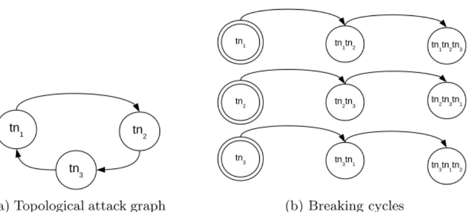
A TAG is a directed graph model defined globally for a system, containing all potential attacks that may happen. It does not contain the position of the at-tacker and thus almost always contains cycles, for example inside local networks in which any host can attack any other one. A simple example of a cycle is shown in Figure 2a.

The common assumption to break cycles in attack graphs is that an attacker will not backtrack, i.e., attack again a node he has already successfully exploited. This is reasonable because backtracking does not bring new attack paths. It has been properly justified by Ammann et al. in [1] and by Liu and Man in [17]. However, the state of the art solutions for Bayesian modelling of an attack graph, such as the ones of Liu and Man [17] and Poolsappasit et al. [25], use this assumption to arbitrarily delete possible attack steps. In reality, in a single model containing all potential attacks, it is impossible to delete cycles without adding new nodes. It would require to know a priori which path the attacker will choose. A solution to break cycles while keeping all possible paths is to enumerate them, starting from all possible attack sources, or targeting all possible targets, keeping in nodes a memory of the path of the attacker. Figure 2b shows an example of such a cycle breaking process. In this figure, the node tn1tn2tn3 means that

Fig. 2. Cycles in a topological attack graph

tn

1 tn2

tn₃

(a) Topological attack graph

tn₁ tn₁tn₂ tn₁tn₂tn₃

tn₂ tn₂tn₃ tn₂tn₃tn₁

tn₃ tn₃tn_{1 tn}

3tn1tn2 (b) Breaking cycles

the attacker controls the node tn3, having first compromised tn1, then tn2. We discuss, in Section 3.4, how we apply this process for Dynamic Risk Correlation Models and, in Section 3.5, for Future Risk Assessment Models. Unfortunately, this process causes a combinatorial explosion in the number of nodes of the model. We also describe in Sections 3.4 and 3.5 how we deal with this challenge in HRAMs, thanks to pruning functions.

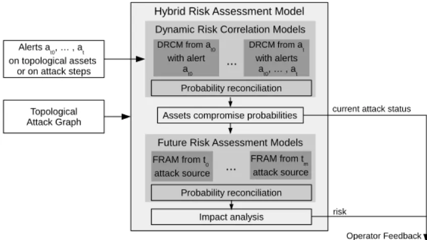
3.3 Hybrid Risk Assessment Model Architecture

Our approach distinguishes two sub-objectives of determining the likelihood of occurrence within dedicated models: Dynamic Risk Correlation Models (DR-CMs) and Future Risk Assessment Models (FRAMs), combined to provide a complete Hybrid Risk Assessment Model (HRAM), whose architecture is pre-sented in Figure 3.

We take as input a TAG generated by an attack graph engine (e.g., Mul-VAL [21] or TVA [12]). First, we build DRCMs from this TAG and the set of current alerts at time t. The reconciliation of the probabilities given by the sev-eral DRCMs gives the current attack status at time t. Then, we build FRAMs which give the likely futures of the system, according to this current status. The combination of these likely futures with an impact analysis results in the risk of the system.

3.4 Dynamic Risk Correlation Model

Building process The goal of the DRCM is to provide explanations for the alerts that have been raised by intrusion detection sensors. By explanation, we mean the identification of the likely source nodes that have been compromised and that have enabled the attacker to launch the detected attack. A DRCM is built from the most recently received alert, the target, and explains why this alert has been generated, taking into account past alerts. As soon as a new alert

Hybrid Risk Assessment Model Topological Attack Graph Operator Feedback Alerts a t0, … , at on topological assets or on attack steps

Assets compromise probabilities

risk

current attack status

Dynamic Risk Correlation Models

Probability reconciliation DRCM from a_t0 with alert a_t0 DRCM from a_t with alerts a_t0, … , a_t ...

Future Risk Assessment Models

FRAM from t₀ attack source FRAM from t_m attack source ... Probability reconciliation Impact analysis

Fig. 3. Hybrid Risk Assessment Model Architecture

is received, a new DRCM is built. Older DRCMs are kept in parallel with the newly generated DRCM, to manage scenarios with several distinct simultaneous attacks (i.e., a new alert is not related to older ones). Probabilities of all kept DRCMs are reconciliated.

Following the process described in Section 3.2, we construct each DRCM in such a way as not to have any cycles, but to keep all possible attack paths “directed to” the target. The DRCM is built from the latest received alert. Then, we recursively add the attack steps and assets allowing to compromise the target. We store, in each DRCM Topological Asset, the path from this node to the target of the DRCM. This allows to ensure that the building process never comes back on a previously exploited node and thus the DRCM does not have cycles, but contains all possible causes of the latest received alert.

Moreover, we design this building process in order to generate a graph struc-ture of the DRCM which is a polytree (i.e., directed graph with no directed nor undirected cycles). This implies, for example, to duplicate the condition and sensor nodes (i.e., new conditions and sensors for each added attack step). The DRCM being a polytree satisfies the requirements of Pearl’s inference algorithm [23], which is quasilinear in the number of nodes. Thus, the inference in such a DRCM with a polytree structure containing duplicated nodes is much more efficient and consume less memory, in comparison with a directed acyclic graph structure with fewer nodes (no duplicates), for identical results.

Model nodes A DRCM is a Bayesian network with 5 types of nodes. Each one represents a Boolean random variable and is associated with a conditional probability table (CPT), representing its probabilistic dependency toward its parents.

– A DRCM Topological Asset represents the random variable describing the status of compromise of a specific asset of the TAG, in order to exploit the DRCM Target. It has one parent (DRCM Attack Step) of each type of attack that can be used to compromise it (i.e., there may be as many parent nodes as there are different attack types) and a DRCM Attack Source representing that this node may be a source of attack. Its CPT is a noisy-OR: at least one successful attack is needed to compromise this node and it can also be compromised if it is the source of attack itself. Even if no parent is compromised, there is still a little chance that an unknown attack compromises this node.

– A DRCM Attack Source represents the random variable describing that a specific asset of the TAG is a source of attack. It is a node without parents. As such, it does not have a complete CPT, but only an a priori probability value. The a priori probability of having an attack coming from this asset has to be set by the operators knowing the probability that an attack starts from this threat source.

– A DRCM Attack Step represents the random variable describing that an attack step has been completed by an attacker. It has two types of parents: DRCM Conditions, and a DRCM Topological Asset. At a minimum, the DRCM Topological Asset is required, but the exact CPT depends on the type of attack step.

– A DRCM Condition represents the random variable describing that the con-dition of an attack step is verified. It does not have any parent. Its a priori probability is the probability of successful exploitation of the condition. – A DRCM Sensor can either be attached to a DRCM Topological Asset or

to a DRCM Attack Step. It represents the random variable describing that the sensor of an attack step or an asset has raised an alert. Its parent is the object monitored by the sensor. Its CPT represents the false-positive and false-negative rates of the sensor. The sensor corresponding to the latest received alert, and from which the DRCM is built, is the target of the DRCM.

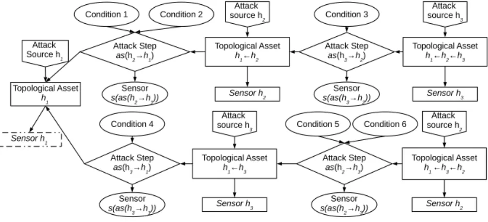
Figure 4 shows an example of a DRCM built from an alert on host h1 (the

node in dotted line on the left) in a topology of 3 hosts. DRCM Topological Assets are represented by a rectangle shape, DRCM Attack Sources by a five-sided shape, DRCM Attack Steps by a diamond shape, and DRCM Conditions by an oval shape.

Model usage As shown in Figure 3, we build the structure of the DRCM according to the TAG, starting from the latest received alert. Then, we set the states of the DRCM Sensors according to the previous security alerts received from the sensors:

– If the sensor of an attack step or an asset exists and is deployed in the network, as long as it has not raised any alert, all related DRCM Sensors are set to the NoAlert state.

Topological Asset h₁←h₂←h₃ Attack Step as(h₃→h₂) Condition 3 Topological Asset h₁  Attack Step

as(h₂→h₁) Topological Asseth₁←h₂ 

Condition 1 Condition 2

Attack Step

as(h₃→h₁) Topological Asseth₁←h₃

Condition 4

Attack Step

as(h₂→h₃) Topological Asseth₁ ←h₃←h₂

Condition 5 Condition 6

Sensor h₁

Attack

source h₂ source hAttack ₃

Attack source h₂ Attack source h₃ Attack Source h₁  Sensor h₂ Sensor h 2 Sensor

s(as(h₂→h₁)) s(as(hSensor₃→h₂)) Sensor h3

Sensor

s(as(h₃→h₁)) Sensor h3 s(as(hSensor₂→h₃))

Fig. 4. Dynamic Risk Correlation Model

– If the sensor has raised an alert corresponding to this attack step or asset, the related DRCM Sensors are set to the Alert state.

– If the attack step or asset has no deployed sensor, there is NoInfo about this sensor. So, the related DRCM Sensors cannot be set in any state and these nodes can be safely deleted from the DRCM, with no impact on other nodes final probabilities.

Then, we use a Bayesian network belief propagation algorithm (e.g., Pearl’s) to update the probabilities of each state at all the nodes.

Probability reconciliation within a DRCM The outputs of a DRCM are of two types: (1) the probabilities of attack sources, describing how likely an asset is to be the source of the attack impacting the target of the DRCM, and (2) the compromise probabilities, describing how likely it is that an asset has been compromised along the path of the attacker.

As a DRCM Topological Asset contains the attack path from its related asset to the target, many DRCM Topological Assets represent the same physical asset. Indeed, the attacker can potentially use several different paths to reach the target: for example, h1 ← h2 ← h4 is different from h1 ← h3 ← h4, but in both cases, the attacker starts from the same asset h4to attack the target h1. In

a DRCM DRCMi, we thus have many DRCM Topological Assets and DRCM

Attack Sources representing the same asset a. We chose to give the operator the worst case for compromise probability of assets. Thus, as output of a DRCM, we assign to an asset:

– a probability of compromise P c that is the maximum of the probabilities of DRCM Topological Assets related to this asset:

– an attack source probability P s that is the maximum of the probabilities of DRCM Attack Sources related to this asset:

P sDRCMi(a) = maxnode∈{DRCM Attack Source(a)}P sDRCMi(node)

Probability reconciliation between DRCMs As described at the begin-ning of Section 3.4, several older DRCMs are kept in parallel with the new ones generated each time a new alert is received. They can be related to different

simultaneous attacks. These DRCMs DRCMi give different sources and

com-promise probabilities for the same asset a. Thus, the second level of probability reconciliation is done between all kept DRCMs. Similarly to the single DRCM case, we want to present the operator with a view of the worst case, and assign to an asset a a probability of compromise P c(a) and an attack source probability P s(a) that is the maximum of the related probabilities in all the DRCMs:

P c(a) = maxDRCMi∈{kept DRCMs}P cDRCMi(a)

P s(a) = maxDRCMi∈{kept DRCMs}P sDRCMi(a)

Pruning in a DRCM The main limitation when implementing the DRCM is the combinatorial explosion of the number of nodes, due to the cycle breaking process. This process introduces a lot of redundancy which increases significantly the size of the model. In order to improve the performance and prevent this combinatorial explosion, we provide a practical way to cut useless paths (with extremely low probabilities) while preserving the other paths.

The probability of a DRCM Topological Asset represents the probability of the attacker having exploited the DRCM target, by exploiting this topological asset. As long as no attack has been detected on a path, the probability of an asset being compromised decreases rapidly as a function of the length of the path between the DRCM Topological Asset and the DRCM Target. Moreover, thanks to the several DRCMs that are kept, if a detected step is discarded in a DRCM, it will be present in another older DRCM, closer to its detection node, thanks to the redundancy of the model. According to the state of the sensors along a path, we have different pruning policies, summarised in Figure 5.

The rules applied when building a DRCM are the following:

– We keep exploring and memorising the path from the target asset, as long as we find Alert sensors.

– For NoAlert sensors, when there are more than MaxNumberNegativeDetec-tionsToExplore, we discard the path and keep only MaxNumberNegativeDe-tectionsToKeep nodes.

– For NoInfo sensors, when there are more than MaxNumberNoInfoToExplore, we discard the path and keep only MaxNumberNoInfoToKeep nodes, but with values for the parameters bigger than for NoAlert sensors.

TN₁  AS1.1 TN1.1 S₁ S AS3.1 S TN3.1 S S AS1.2 TN1.2 S S AS1.3 TN1.3 S S AS1.4 TN1.4 S S AS3.2 S TN3.2 S MaxNumberNoInfoToKeep = 4 MaxNumberNoInfoToExplore = 8 MaxNumberNegativeDetectionsToKeep = 2 MaxNumberNegativeDetectionsToExplore = 4 AS2.1 TN2.1 S S AS2.2 TN2.2 S S AS2.3 TN2.3 S S AS2.4 TN2.4 S S

Caption: ×: NoAlert sensor; X: Alert sensor; ?: NoInfo sensor

Fig. 5. Pruning policies in Dynamic Risk Correlation Model

– As soon as an Alert sensor is found on an explored path, the counters of NoAlert and NoInfo are reset to 0.

Thus, the parameter MaxNumberNegativeDetectionsToExplore corresponds to the maximum number of successive false-negatives (missed detections) that we allow the model to take into account. The parameter MaxNumberNoInfoToKeep corresponds to the maximum number of successive undetectable steps that we allow the model to take into account.

Selection of the DRCMs to keep The last important thing about this model is the selection of the DRCMs to keep. Indeed, as one new DRCM is generated each time an alert is received, the number of models to keep can increase quickly. However, when several alerts are part of the same attack, they will be part of the DRCM whose target is the sensor that raised the latest alert. Moreover, there will be more Alert sensors in this DRCM (increasing probabilities of all nodes of the DRCM), and at most the same number of NoAlert sensors (decreasing probabilities) than in all previous DRCMs related to the same attack. Thus, all the previous DRCMs related to the same attack are useless, because they are included in the last generated DRCM and their probabilities will be lower so they do not change the maximum of asset compromise probabilities. The only different DRCMs that are useful to keep are those not related to the same attacks because they bring new information about the occurring attacks. They can be identified by having at least one DRCM Topological Asset, with a higher probability than all the ones of the latest DRCM, for the same asset. These attacks could be part of a more global attack scenario, starting from different sources, that has not yet converged or it might be distinct attacks that are happening simultaneously. That is why we may need to keep several DRCMs in parallel.

3.5 Future Risk Assessment Model

Building process and model usage The second type of model constituting the HRAM is the Future Risk Assessment Model (FRAM). The goal of such model is to evaluate among all possible futures, the ones that are the most likely to happen. As indicated by Figure 3, a FRAM is built from each attack source, according to the DRCMs’ reconciled compromise probabilities. Then, we use a belief propagation algorithm to update the probabilities of all the nodes. When there is a completed attack step or a compromised asset, a FRAM taking this node as starting point is built or updated and the branches from this attack step are deleted in all other FRAMs. Indeed, this attack is no longer a possible future, as it has happened and will be investigated in its own FRAM. Even if the structure of a FRAM does not change with detections, its probabilities of conditions and attack sources can be updated. For example, the condition probability of a vulnerability that has already been exploited is set to ”1”.

The way FRAMs are built and cycles solved is identical to the DRCMs, starting from an attack source rather than from a target. See Sections 3.2 and 3.4 for more details.

Model nodes A FRAM is a Bayesian Network with 5 types of nodes, each one representing a Boolean random variable. Each node is associated with a conditional probability table (CPT), representing its probabilistic dependency toward its parents.

– A FRAM Topological Asset represents the random variable describing the future status of compromise of an asset of the TAG. Its CPT is the same as DRCM Topological Assets without the DRCM Attack Source parent. – The FRAM Attack Source represents the random variable describing that

an asset is the source of attack. It is the root of the FRAM. It does not have any parent and its a priori probability is provided by the reconciliation of probability of DRCMs.

– A FRAM Attack Step represents the random variable describing that an attack step can be successfully exploited by an attacker. Its CPT is the same as DRCM Attack Steps.

– A FRAM Condition represents the random variable describing that the con-dition of an attack step is verified. Its a priori probability is the same as DRCM Conditions.

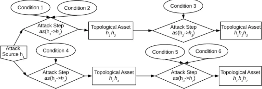
Figure 6 shows an example of a Future Risk Assessment Model starting from

host h1 in a topology of 3 hosts. The FRAM Attack Source is represented by a

five-sided shape, FRAM Topological Assets by a rectangle shape, FRAM Attack Steps by a diamond shape, and FRAM Conditions by an oval shape.

Probability reconciliation in FRAMs Similarly to the DRCM, several FRAM Topological Assets can represent the same topological asset, when an attacker can use several paths. We chose to give to the operator the worst case,

Topological Asset h₁h₂h₃ Attack Step as(h₂->h₃) Condition 3 Attack Step as(h1->h2) Topological Asset h₁ h₂ Condition 1 Condition 2 Attack Step

as(h₁->h₃) Topological Asseth₁ h₃

Condition 4

Attack Step

as(h₃->h₂) Topological Asseth₁ h₃h₂

Condition 5 Condition 6 Attack

Source h1 

Fig. 6. Future Risk Assessment Model

for the probability of the assets being compromised in the near future, just like in DRCMs. Thus, as output of a FRAM, we assign to an asset a probability of compromise in the future that is the maximum of the probabilities of FRAM Topological Assets targeting the same asset.

Pruning in a FRAM As a FRAM does not include any evidence (i.e., it does not contain sensor nodes which are set in a specific state), the Bayesian inference is much easier to compute. Moreover, it has fewer nodes than a DRCM, thus its combinatorial explosion of nodes is not as important. However, the combinatorial explosion of the number of nodes, due to the cycle breaking process is still present. If they are not built carefully, there is a lot of useless redundancy in all FRAMs, which increases significantly the size of the model. A major part of this redundancy can be deleted when building a new FRAM, by deleting all the paths started from all sources of other FRAMs. All these subtrees can be deleted safely, as their probabilities will be less than the probabilities of the FRAM started from the attack source. Moreover, as we only want to predict the near future, we can limit to a small number of steps (e.g., 3) the next steps to compute.

3.6 Impact analysis

The last component necessary to build our Hybrid Risk Assessment Model is the impact analysis function. The goal of this function is to take the assets of the information systems with their compromise likelihood computed by the FRAMs and an impact score associated with each asset to give a risk score to assets. We apply the usual equation to compute the risk R of a topological asset a, with the probability of compromise P of the asset computed by the FRAMs, and the impact I of its compromise:

R(a) = P (a) × I(a)

In this work we focus on the likelihood computation (P (a)), whose method-ology is independent of the system studied, whereas the impact analysis (I(a))

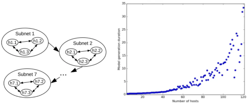
Subnet 1 h1.1 h1.2 h1.3

...

(a) Simulations network topology (b) HRAM performance evaluation (seconds) Fig. 7. Simulations of the Hybrid Risk Assessment Model

strongly depends on the organisation. Thus, we only associated with each asset a fixed impact score. Moreover, in order to validate the probabilistic results of the model, we assign to each asset the same impact value (I(a) = 1, ∀a) for the validation.

4

Validation

As a use case, to validate the performances and the results of the HRAM, we simulate network topologies, as shown in Figure 7a, containing up to 120 hosts, divided in 7 subnets. These topologies are representative of a real network in which defence in depth is implemented: all the hosts of a subnet have access to all the hosts of a deeper subnet. In each subnet, all accesses between hosts are authorised. Each host has 30 random vulnerabilities for a maximum total of around 3600 vulnerabilities.

4.1 Performances

To evaluate the performances of the model, we first generate the topological attack graphs of the simulated topologies . Then, for each simulation, we generate one random attack scenario of 7 successive attack steps , to which are added false positives and steps with no sensor information. Finally, we evaluate the HRAM. Figure 7b shows the duration in seconds of the generation of the HRAM (TAG generation then DRCM and FRAM) on such topologies, with one scenario of 7 attack steps. This simulation shows that for medium-sized topologies (up to 120 hosts) the duration of the HRAM analysis is sufficiently small (< 35 seconds), for the operator to be able to properly understand the risk in operational time.

(a) DRCM accuracy evaluation (b) FRAM accuracy evaluation Fig. 8. Accuracy of the Hybrid Risk Assessment Model

This could be extended to bigger information systems, by clustering together identical (in terms of vulnerabilities, roles, permissions, network accesses, etc.) templates of servers or of client machines in one topological asset, as they possess the same vulnerabilities and authorised accesses and thus behave in a similar way in the HRAM. Even with 60 assets in the topological attack graph with, for example, 20 templates of client machines, 15 of network servers, and 25 of business application servers, it is possible to model a real world large company information system.

4.2 Accuracy

To evaluate the accuracy of the results of the DRCMs (i.e., how close the com-promise probabilities are from the truth), we simulate attack scenarios of up to 7 successive steps on random topologies of 70 hosts, as presented in Section 4.1 (results are identical from 10 up to 120 hosts). We add to the 7 true positive alerts of these scenarios, 10 randomly located false positives and 10 sensors with no information (i.e., a positive predictive value of P P V = ₇₊₁₀7 ≈ 0.4).

The results of these simulations are shown in Figure 8a. For each simulated scenario, we compare the theoretical results known in the scenarios with the re-sults obtained as output of the DRCM started from the lastly raised alert. In the plot of Figure 8a, the black curve on the top represents the compromise prob-abilities, with a confidence interval, during 10 simulations, of the hosts known as compromised in the scenarios, according to the number of attack steps in the scenario. The theoretical result would be a line with only ”1” probabilities. The grey curve at the bottom represents the compromise probabilities, with a confi-dence interval, during 10 simulations, of the hosts known as healthy, according to the number of attack steps in the scenario. The theoretical result would be a line with only ”0” probabilities. Note that after 3 attack steps in the scenario

for the compromised hosts, and for all values for not compromised hosts, the confidence interval is so small that it cannot be noticed on the figure.

This experimentation shows that the greater the number of attack steps in the scenario, the larger the recognition probability and the smaller the confidence interval. Moreover, it shows a large free space between the curve of compromised hosts and the curve of healthy hosts. This means that there are no false negative and false positive introduced by the DRCM. Finally, even if there are false-positives and sensors without information, compared to the number of successive attack steps (up to 7), we retrieve only the real attack elements, thanks to our model built from the latest received alert and taking into account the order and relations between attack steps.

We use the same simulated topologies to evaluate the accuracy of the results of the FRAMs (i.e., how close the possible futures are from the next step of attack). The results of these simulations are shown in Figure 8b. We compare the next attack step known in each scenario with the results obtained as output of the FRAM started from the previous scenario (with one less attack step). In the plot of Figure 8b, the black curve on the top represents the future risk probability computed by the FRAM of the future attack step (known in the next attack scenario). The grey curve on the bottom represents the average future risk probabilities, computed by the FRAM, of all other hosts of the topology, with confidence intervals.

This experimentation shows that the FRAM predicts quite well the next step of attack in the simulated scenarios, because its probability is generally much higher than the probabilities of other next steps . However, this is possible because in these simulations, the attacker takes the easiest attack steps (i.e., attacks the most vulnerable machine) The FRAM is thus particularly interesting when few future attack steps are easier than the other possible futures.

5

Related Work

Many people have proposed enhancements to improve attack graphs or trees with Bayesian networks, in order to use them for dynamic risk assessment [26,17,27]. However, they do not describe accurately how they address cycles that are in-herent to attack graphs. For example, in [27], Xie et al. present an extension of MulVAL attack graphs, using Bayesian networks, but they do not mention how to manage the cycle problem, while MulVAL attack graphs frequently contain cycles. In the same way, in [7], Frigault and Wang do not mention how they deal with the cycle problem when constructing Bayesian attack graphs. In [17], Liu and Man assert that to delete cycles, they assume that an attacker will never backtrack. Poolsappasit et al. in [25] use the same hypothesis. However, as de-tailed in Section 3.2, they do not present how they deal with this hypothesis to keep all possible paths in the graph, while deleting cycles. We propose here novel models exploding cycles in the building process, in order to keep all possible paths, while deleting the cycles, to compute the Bayesian inference. Moreover, we also add several improvements (practical pruning, polytree structure, etc.)

reducing the size of the graph structure and improving the performance of the inference. We thus constrain the size of the graph in which we do Bayesian inference, while conserving all paths by linearising cycles.

The model presented by Xie et al. [27] and the one of Liu and Man [17] are made of a single model to describe the compromise status of assets of the infor-mation system. In a single model, an increase of compromise probability of an asset due to an already happened attack is mixed up with an increase due to a very likely possible future. However, the distinction of these two causes is very valuable for a security operator, for example to select where to deploy a reme-diation. The hybrid model we propose separates the compromise information of the past alerts from those of the likely futures. It allows a security operator to know if a topological asset has already been compromised (thanks to DRCMs) or if it may be compromised in the near future (FRAMs).

In this work, we focus on the likelihood component of the risk assessment. Thus, we use a simple impact function as output of the FRAMs, matching each compromised topological asset with a fix impact value. Other works of the state of the art rather focus on the impact component. For example, Kheir et al. in [13] details how to use a dependency graph to compute the impact of attacks on Confidentiality, Integrity and Availability. This work is complementary to ours as we could add this kind of impact function after the FRAMs to compute a more accurate attack impact.

Models such as [8] use Dynamic Bayesian Networks to monitor and predict the future status of the system. It uses a sequence of Bayesian networks, which can be huge to process. The model we propose here keeps only the past in-formation necessary to explain all alerts and to update the models to evaluate potential futures (FRAMs). Moreover, the building process and exploitation of DRCMs takes into account the temporality of raised alerts to determine attacks. Finally, contrary to other models based on Bayesian attack graphs, our model can distinguish several distinct simultaneous attacks in the alerts raised in a system, by analysing all kept DRCMs .

Our experimental validation uses simulated topologies far bigger than the state of the art. For example, Xie et al. assess their model on 3 hosts and 3 vulnerabilities [27], Liu and Man on 4 hosts and 8 vulnerabilities [17]. The real world examples used by Frigault and Wang in [7] contain at most 8 vulnerabilities on 4 hosts. The test network used by Poolsappasit et al. in [25] contains 8 hosts in 2 subnets, but with only 13 vulnerabilities. Thanks to our polytree models, we successfully run our HRAM efficiently on simulated topologies with up to 120 hosts for a total of more than 3600 vulnerabilities.

6

Conclusion and Future Work

We present in this paper a new Hybrid Risk Assessment Model, combining the dynamic risk correlation and the future risk assessment analysis. This model enables dynamic risk assessment. It is built from a topological attack graph, using already available information. Dynamic Risk Correlation Models are built

according to dynamic security events, to update the compromise probabilities of assets. We use these probabilities to build Future Risk Assessment Models, to compute the most likely futures. This combination of two complementary models separates the compromise status of assets between past attacks and likely futures. This model handles the cycles in attack graphs and thus is applicable to any information system, with multiple potential attack sources. The cycle breaking process significantly increases the number of nodes in the model, but thanks to the polytree structure of the Bayesian networks we build and practical pruning, the inference remains efficient, for big information systems. In order to be able to use the Hybrid Risk Assessment Model for even bigger information systems, future work will investigate how the usage of a hierarchical topological attack graph can be appropriate to build the Hybrid Risk Assessment Model. Another future work will be to use the ability of Bayesian networks to learn parameters from data, in order to update the values in the Conditional Probability Tables after the confirmation/negation of compromise by the operators.

References

1. Ammann, P., Wijesekera, D., Kaushik, S.: Scalable, graph-based network vulner-ability analysis. In: Proceedings of the 9th ACM Conference on Computer and Communications Security. pp. 217–224. ACM (2002)

2. Artz, M.L.: Netspa: A network security planning architecture. Ph.D. thesis, Mas-sachusetts Institute of Technology (2002)

3. Ben-Gal, I., Ruggeri, F., Faltin, F., Kenett, R.: Bayesian networks, encyclopedia of statistics in quality and reliability (2007)

4. Cole, R.: Multi-step Attack Detection via Bayesian Modeling Under Model Param-eter Uncertainty. Ph.D. thesis, The Pennsylvania State University (2013)

5. de la D´efense Nationale, S.G.: Ebios-expression des besoins et identification des objectifs de s´ecurit´e (2004)

6. Forum of Incident Response and Security Teams: Common vulnerability scoring system v3.0: Specification document. pp. 1–21 (2015)

7. Frigault, M., Wang, L.: Measuring network security using bayesian network-based attack graphs pp. 698–703 (July 2008)

8. Frigault, M., Wang, L., Singhal, A., Jajodia, S.: Measuring network security using dynamic bayesian network. In: Proceedings of the 4th ACM workshop on Quality of protection. pp. 23–30. ACM (2008)

9. ISO, I., Std, I.: Iso 27005: 2011. Information technology–Security techniques– Information security risk management. ISO (2011)

10. ISO/IEC 27000:2014: Information technology – Security techniques – Information security management systems – Overview and vocabulary. Tech. rep. (2014) 11. Jajodia, S., Noel, S., O’Berry, B.: Topological analysis of network attack

vulnera-bility. Managing Cyber Threats pp. 247–266 (2005)

12. Jajodia, S., Noel, S., Kalapa, P., Albanese, M., Williams, J.: Cauldron mission-centric cyber situational awareness with defense in depth. In: Military Communi-cations Conference. pp. 1339–1344. IEEE (2011)

13. Kheir, N., Debar, H., Cuppens-Boulahia, N., Cuppens, F., Viinikka, J.: Cost eval-uation for intrusion response using dependency graphs. In: Network and Service Security, 2009. N2S’09. International Conference on. pp. 1–6. IEEE (2009)

14. Kordy, B., Pi`etre-Cambac´ed`es, L., Schweitzer, P.: DAG-based attack and defense modeling: Don’t miss the forest for the attack trees. Computer science review 13, 1–38 (2014)

15. Lauritzen, S.L., Spiegelhalter, D.J.: Local computations with probabilities on graphical structures and their application to expert systems. Journal of the Royal Statistical Society (1988)

16. Lippmann, R.P., Ingols, K.W.: An annotated review of past papers on attack graphs. Tech. rep., DTIC Document (2005)

17. Liu, Y., Man, H.: Network vulnerability assessment using bayesian networks. In: Defense and Security. pp. 61–71. International Society for Optics and Photonics (2005)

18. National Information Assurance Glossary: CNSS N 4009: Committee on National Security Systems. Tech. rep. (2010)

19. National Institute of Standards and Technology: SP 800-30 Rev. 1: Guide for Con-ducting Risk Assessments. Tech. rep. (2012)

20. National Institute of Standards and Technology: SP 800-53 Rev. 4: Security and Privacy Controls for Federal Information Systems and Organizations. Tech. rep. (2013)

21. Ou, X., Govindavajhala, S., Appel, A.W.: Mulval: A logic-based network security analyzer. In: USENIX Security Symposium (2005)

22. Pearl, J.: Fusion, propagation, and structuring in belief networks. Artificial intel-ligence 29(3), 241–288 (1986)

23. Pearl, J.: Probabilistic reasoning in intelligent systems: networks of plausible in-ference. Morgan Kaufmann (1988)

24. Phillips, C., Swiler, L.P.: A graph-based system for network-vulnerability analysis (1998)

25. Poolsappasit, N., Dewri, R., Ray, I.: Dynamic security risk management using bayesian attack graphs. Dependable and Secure Computing (2012)

26. Qin, X., Lee, W.: Attack plan recognition and prediction using causal networks. In: Computer Security Applications Conference. pp. 370–379 (Dec 2004)

27. Xie, P., Li, J.H., Ou, X., Liu, P., Levy, R.: Using bayesian networks for cyber security analysis. In: IEEE/IFIP International Conference on Dependable Systems and Networks. pp. 211–220. IEEE (2010)