www.atmos-chem-phys.net/7/377/2007/ © Author(s) 2007. This work is licensed under a Creative Commons License.
Chemistry
and Physics
Comparisons between ground-based FTIR and MIPAS N
2
O and
HNO
3
profiles before and after assimilation in BASCOE
C. Vigouroux1, M. De Mazi`ere1, Q. Errera1, S. Chabrillat1, E. Mahieu2, P. Duchatelet2, S. Wood3, D. Smale3, S. Mikuteit4, T. Blumenstock4, F. Hase4, and N. Jones5
1Belgian Institute for Space Aeronomy (BIRA-IASB), Brussels, Belgium
2Institut d’Astrophysique et de G´eophysique, University of Li`ege (ULg), Li`ege, Belgium 3National Institute for Water and Atmospheric Research (NIWA), Lauder, Otago, New-Zealand
4Institute of Meteorology and Climate Research (IMK), Forschungszentrum Karlsruhe and University of Karlsruhe, Karlsruhe, Germany
5University of Wollongong, Wollongong, Australia
Received: 29 May 2006 – Published in Atmos. Chem. Phys. Discuss.: 1 September 2006 Revised: 7 December 2006 – Accepted: 14 January 2007 – Published: 23 January 2007
Abstract. Within the framework of the Network for
Detec-tion of Atmospheric ComposiDetec-tion Change (NDACC), reg-ular ground-based Fourier transform infrared (FTIR) mea-surements of many species are performed at several loca-tions. Inversion schemes provide vertical profile informa-tion and characterizainforma-tion of the retrieved products which are therefore relevant for contributing to the validation of MIPAS profiles in the stratosphere and upper troposphere. We have focused on the species HNO3 and N2O at 5 NDACC-sites distributed in both hemispheres, i.e., Jungfraujoch (46.5◦N) and Kiruna (68◦N) for the northern hemisphere, and
Wol-longong (34◦S), Lauder (45◦S) and Arrival Heights (78◦S)
for the southern hemisphere. These ground-based data have been compared with MIPAS offline profiles (v4.61) for the year 2003, collocated within 1000 km around the stations, in the lower to middle stratosphere. To get around the spatial collocation problem, comparisons have also been made be-tween the same ground-based FTIR data and the correspond-ing profiles resultcorrespond-ing from the stratospheric 4D-VAR data assimilation system BASCOE constrained by MIPAS data. This paper discusses the results of the comparisons and the usefullness of using BASCOE profiles as proxies for MIPAS data. It shows good agreement between MIPAS and FTIR N2O partial columns: the biases are below 5% for all the sta-tions and the standard deviasta-tions are below 7% for the three mid-latitude stations, and below 10% for the high latitude ones. The comparisons with BASCOE partial columns give standard deviations below 4% for the mid-latitude stations to less than 8% for the high latitude ones. After making some corrections to take into account the known bias due to the use of different spectroscopic parameters, the comparisons Correspondence to: C. Vigouroux
(Corinne.Vigouroux@bira-iasb.oma.be)
of HNO3 partial columns show biases below 3% and stan-dard deviations below 15% for all the stations except Arrival Heights (bias of 5%, standard deviation of 21%). The re-sults for this species, which has a larger spatial variability, highlight the necessity of defining appropriate collocation criteria and of accounting for the spread of the observed air-masses. BASCOE appears to have more deficiencies in pro-ducing proxies of MIPAS HNO3profiles compared to N2O, but the obtained standard deviation of less than 10% between BASCOE and FTIR is reasonable. Similar results on profiles comparisons are also shown in the paper, in addition to par-tial column ones.
1 Introduction
MIPAS, Michelson Interferometer for Passive Atmospheric Sounding1(Fischer and Oelhaf, 1996; ESA, 2000), is one of the 10 instruments on board the European satellite ENVISAT which was launched into a sun-synchronous polar orbit at 800 km altitude, on March 1, 2002. This Fourier transform spectrometer operates in the mid infrared (4.15–14.6 µm or 685–2410 cm−1) and measures high-resolution (0.025 cm−1 unapodised) radiance spectra at the Earth’s limb. It provides day and night vertical profiles of a large number of atmo-spheric species with a complete global coverage of the Earth obtained in 3 days.
Part of the validation of the MIPAS Level 2 products is performed within the ENVISAT Stratospheric Aircraft and Balloon Campaigns (ESABC) or by comparisons with data from other limb sounding instruments such as HALOE (the
HALogen Occultation Experiment on UARS, the Upper At-mosphere Research Satellite2). Additional independent mea-surements for the validation of MIPAS are perfomed by the ground-based Fourier transform infrared (FTIR) solar ab-sorption spectrometers, like those operated in the framework of the Network for the Detection of Atmospheric Composi-tion Change (NDACC3, formerly called NDSC, Network for the Detection of Stratospheric Change). The implementa-tion of the Optimal Estimaimplementa-tion Method, described in Rodgers (2000), in the inversion schemes of the ground-based FTIR spectra allows the retrieval of low resolution vertical pro-file information (in addition to the standard total column amounts), and the characterization of the retrieved products. When it comes to verifying the MIPAS profiles at their full vertical resolution, the FTIR data cannot compete with the high vertical resolution measurements coming from balloon, aircraft or limb sounding satellite experiments. The partic-ular benefit of using ground-based FTIR data lies in the fact that these measurements are performed regularly under clear-sky conditions, at many stations distributed over the globe, and thus represent a very interesting complementary data set for performing a statistically sound validation, and for moni-toring the quality of the MIPAS products on the longer term. These ground-based FTIR data are therefore useful for con-tributing to the validation of MIPAS profiles in the strato-sphere and upper tropostrato-sphere.
Some preliminary results of MIPAS validation by bal-loon, aircraft, satellite, ground-based measurements, and data assimilation systems (including BASCOE) have been presented in the second workshop on Atmospheric Chem-istry Validation of Envisat (ACVE-2) in May 2004 (ESA, 2004a) for all the MIPAS ESA Level 2 products, that are the vertical profiles of: temperature, H2O, O3, NO2, CH4, N2O (Camy-Peyret et al., 2004), and HNO3 (Oel-haf et al., 2004). In the present study, we focus on a more advanced validation of the MIPAS ESA products for the year 2003, for N2O and HNO3, a tropospheric source species and a stratospheric reservoir species respectively, for which the FTIR technique is the only available ground-based source of data during the considered period of MI-PAS operations. Five NDACC stations are involved in this work: Kiruna (67.8◦N, 20.4◦E, altitude 420 m a.s.l.) and Jungfraujoch (46.5◦N, 8.0◦E, 3580 m a.s.l.) in the northern hemisphere, and Wollongong (34.4◦S, 150.9◦E, 30 m a.s.l.), Lauder (45.0◦S, 169.7◦E, 370 m a.s.l.), and Arrival Heights (77.8◦S, 166.7◦E, 200 m a.s.l.) in the southern hemisphere.
This paper describes in Sect. 2 the MIPAS ESA Level 2 products and, in Sect. 3, the ground-based FTIR vertical pro-file data, including some information concerning the retrieval strategies used at each station and the characterization of the data products. BASCOE, a 4D-VAR chemical data assim-ilation system, is described in Sect. 4. In the subsequent
2http://haloedata.larc.nasa.gov/home/ 3http://www.ndacc.org/
section, we explain the adopted methodology for the com-parisons for which two approaches have been used. First, we have made the comparisons with the MIPAS offline profiles (v4.61) provided by ESA, taking care to define reasonable collocation criteria that give enough coincidences to obtain relevant statistics. Then, to improve the collocations without decreasing the number of coincidences, we have compared the ground-based FTIR profiles with the products of BAS-COE. In the current configuration, BASCOE is constrained with MIPAS data and thus delivers atmospheric profiles that can be considered to be proxies of the MIPAS profiles, at any location and any time. In the last part (Sect. 6), we show the results obtained from the comparisons for both molecules, N2O and HNO3, at the different stations, and try to answer the following two questions: (1) can we quantify the agree-ment between the MIPAS and the ground-based FTIR data, and (2), what are the benefits of using the results of a data assimilation system as proxies of MIPAS profiles instead of the MIPAS profiles themselves?
2 MIPAS data
The MIPAS Level 2 products are described in the MIPAS Product Handbook4 and in Raspollini et al. (2006). The MIPAS offline data used here were provided by the ESA v4.61 data processor (ESA, 2004b). They include the N2O and HNO3volume mixing ratio (vmr) profiles as well as the atmospheric pressure and temperature vertical distributions. The vertical resolution of the delivered profiles is between 3 and 4 km and their horizontal resolution is between 300 and 500 km along track.
The individual MIPAS profiles do not cover the same al-titude ranges. We observed that, for the scans used in the present study, the upper altitude limits of given MIPAS vmr profiles are quite constant for all profiles: they are around 61 km for N2O and 43 km for HNO3. The lower limits vary a lot between a minimum of 6 km for N2O and 9 km for HNO3 to greater than 20 km for worst cases. The latter variability is due to the presence of clouds: the retrievals of trace gas concentrations are limited to altitudes above the cloud top height (for clouds with high opacity in the infrared). The highest cloud heights are found, as expected, in the tropical upper troposphere (sub-visible cirrus) and in the Antarctic polar vortex (polar stratospheric clouds) (Raspollini et al., 2006). To avoid the need to extrapolate MIPAS profiles be-yond the altitude limits for which retrieved vmr values are provided, while keeping a statistically relevant data set, we have restricted the considered MIPAS data set to the scans for which the lower altitude limit is smaller than or equal to 12 km for N2O and 14 km for HNO3. This option will allow us to consider partial column values consistently above 12 km for N2O and above 14 km for HNO3, without including
Table 1. Spectral microwindows (cm−1) used for the ground-based FTIR retrievals.
N2O HNO3
Station Microwindow Interfering species Microwindow Interfering species
limits (cm−1) limits (cm−1) Kiruna 2481.3−2482.6 CO2, CH4, H2O, O3 867.0−869.6 OCS, H2O, CO2, C2H6, CCl2F2 2526.4−2528.2 CO2, CH4, H2O, O3 872.8−875.2 OCS, H2O, CO2, C2H6, CCl2F2 2537.85−2538.8 CO2, CH4, H2O, O3 2540.1−2540.7 CO2, CH4, H2O, O3 Jungfraujoch 2481.3−2482.6 CO2, CH4 868.476−870.0 OCS, H2O 2526.4−2528.2 CO2, CH4, HDO 2537.85−2538.8 CH4 2540.1−2540.7 none Wollongong 2481.2−2483.5 CO2, CH4 868.47−870.0 OCS, H2O, NH3, CO2 872.8 − 874.0 OCS, H2O, NH3, CO2
Lauder & Arrival Heights 2481.2−2483.5 CO2, CH4 868.3−869.6 OCS, H2O, NH3 872.8 − 874.0 OCS, H2O, NH3
extrapolated values. However, some scans can have one or two missing values that are replaced by interpolated values in the profiles.
Because of possible uncertainties in the referencing of the MIPAS profiles versus altitude (Raspollini et al., 2006), we have adopted a vertical pressure grid for making the com-parisons. Daily pressure data from each station have been used to convert the FTIR altitude grid (that covers the alti-tude range from the local surface altialti-tude to about 100 km) to a unique pressure grid. The MIPAS retrieved profiles were interpolated onto the same pressure grid.
3 Ground-based FTIR data
3.1 Retrieval algorithms
Vertical profile informations can be obtained from high-resolution FTIR solar occultation spectra thanks to the pres-sure broadening of the absorption lines which leads to an alti-tude dependence of the lineshapes. Two different algorithms have been used in the present work, SFIT2 and PROFFIT9. Both codes are based on a semi-empirical implementation of the Optimal Estimation Method developed by Rodgers (2000) and provide the retrieval of molecular vertical profiles by fitting one or more narrow spectral intervals (microwin-dows). The SFIT2 algorithm has been described in previous works (Pougatchev and Rinsland, 1995; Pougatchev et al., 1995; Rinsland et al., 1998). It was used for the spectral in-version of the FTIR data at all stations except Kiruna. The profiles of this latter station have been retrieved using the PROFFIT9 algorithm (Hase, 2000). It has been shown re-cently (Hase et al., 2004) that the retrieved profiles and total
column amounts obtained by these two different algorithms under identical conditions are in excellent agreement (within 1% for total column amounts of N2O and HNO3).
In both codes SFIT2 and PROFFIT9, the retrieved state vector contains the retrieved volume mixing ratios of the tar-get gas defined in discrete layers in the atmosphere, as well as the retrieved interfering species column amounts, and fit-ted values for some model parameters. These can include the baseline slope and instrumental lineshape parameters such as an effective apodization. For the stations Jungfraujoch, Wollongong, Lauder and Arrival Heights, the atmosphere is divided in 29 layers, whereas for Kiruna it is divided in 44 layers. The 29 layers have a width of 2 km below 50 km, becoming progressively larger towards the top of the atmo-sphere, defined here as 100 km. The widths of the 44 layers of Kiruna progressively grow from 0.4 km at the ground to 2.3 km around 50 km altitude.
3.2 Retrieval parameters
The characteristics of the FTIR retrieval results are deter-mined by the selection of microwindows, a priori informa-tions, as well as additional model parameters and retrieval parameter settings. The purpose of this work is not to com-pare the FTIR results among them, but to show whether there is an agreement between MIPAS and independent FTIR data at different locations. Except for a common choice of the a priori profiles of the two target gases (see Sect. 3.2.2 here-after), the FTIR retrievals have been made independently at each contributing station, with retrieval parameter settings chosen such as to optimise the retrieval results. What is im-portant in the further comparisons is that we take into
ac-0 0.05 0.1 0.15 0.2 0.25 0.3 0.35 0 10 20 30 40 50 60 70 vmr (ppmv) Altitude (km)
A priori profiles for N2O Kiruna
Jungfraujoch Jan − Mar Jungfraujoch Apr − Sep Jungfraujoch Oct − Dec Arrival Heights Jan − Mar Arrival Heights Apr − Sep Arrival Heights Oct − Dec Lauder, Wollongong Jan − Mar Lauder, Wollongong Apr − Sep Lauder, Wollongong Oct − Dec
0 0.002 0.004 0.006 0.008 0.01 0.012 0.014 0 10 20 30 40 50 60 70
A priori profiles for HNO3
vmr (ppmv)
Altitude (km)
Kiruna
Jungfraujoch Jan − Mar Jungfraujoch Apr − Sep Jungfraujoch Oct − Dec Arrival Heights Jan − Mar Arrival Heights Apr − Sep Arrival Heights Oct − Dec Lauder, Wollongong Jan − Mar Lauder, Wollongong Apr − Sep Lauder, Wollongong Oct − Dec
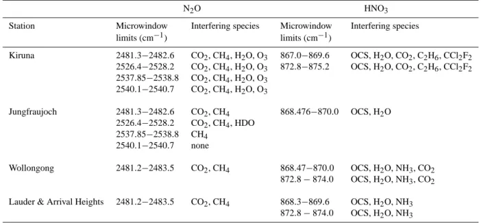
Fig. 1. N2O and HNO3a priori profiles at all stations.
count the individual characteristics of the retrieval results, expressed in the averaging kernels and associated degrees of freedom for signal (DOFS), as discussed further in Sect. 3.3. Also, it is useful to know which spectroscopic data have been used in the FTIR retrievals, to have a better insight in possi-ble biases associated herewith.
3.2.1 Spectroscopic data and spectral windows
All stations are using the spectroscopic line parameters from the HITRAN 2000 database including official updates through 2001 (Rothman, 2003). Wollongong added official updates up to August 2002 and additional lines from the Spectroscopic Atlas of Atmospheric Microwindows in the Middle Infra-Red (2nd edition) (Meier et al., 2004) but these do not include changes in the parameters for N2O or HNO3, or for the six interfering species, given in Table 1, that are fitted in Wollongong retrievals.
At all stations daily temperature and pressure profiles have been taken from the National Centers for Environmental Pre-diction (NCEP).
The retrieval microwindows used at the various stations are listed in Table 1, together with the corresponding interfer-ing species. The a priori profiles of these interferinterfer-ing species are scaled simultaneously with the profile inversion of the target gases in the spectral fit procedure. Depending on lo-cation and altitude of the site and on spectral characteristics, the impact on the retrievals of fitting additional interfering species can be more or less significant. This explains why we do not always find the same interferers in the same mi-crowindows.
3.2.2 A priori profile information
Because the inversion problem is ill-posed, the Optimal Es-timation Method needs some a priori information about the retrieval state vector parameters, including the a priori ver-tical vmr profile xa, and the associated a priori covariance
matrix Sa(Rodgers, 2000).
In Fig. 1, we show the a priori N2O and HNO3 vertical profiles used at each station. For the stations Jungfraujoch, Lauder, Arrival Heights and Wollongong, the a priori profiles have been taken identical to the climatological initial guess profiles from MIPAS for the corresponding seasons and lat-itude bands (so-called IG2 profiles in the MIPAS Product Handbook). Three different seasonal profiles are used, repre-sentative of the periods January to March, April to September and October to December.
For the Kiruna station, only one a priori profile is used for each species, namely the MIPAS IG2 profile for the April to September season corresponding to the latitude of Kiruna. For HNO3at Kiruna, the MIPAS IG2 profile has been mod-ified below 30 km because it was found more realistic to en-hance the a priori amount of HNO3near the tropopause.
As explained above, we do not give individual retrieval parameters such as the Sa matrices: we prefer to give the
characterization of the retrieval results because that is the in-formation that is used in the comparisons.
3.3 Characterization of the retrievals
As discussed in Rodgers (2000), the Optimal Estimation Method allows the characterization of the retrievals, i.e., the vertical resolution of the retrieval, its sensitivity to the a priori information and the DOFS. This is obtained by considering that the retrieved state vector xr is related to the true state
−0.20 0 0.2 0.4 0.6 0.8 1 1.2 10 20 30 40 50 60
Mixing Ratio Averaging Kernel
Altitude [km] 33 km 29 km 25 km 21 km 17 km 13 km 9 km 5 km 1.1 km Sensitivity
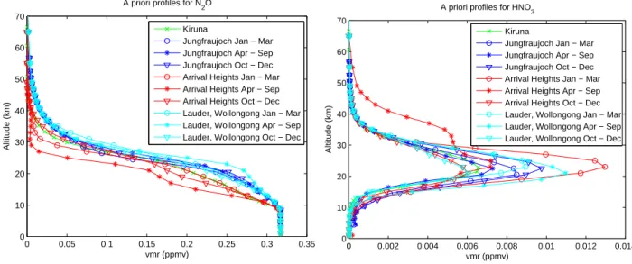
Fig. 2. Characterization of the retrieval of N2O at Arrival Heights.
Full and dashed lines: Volume mixing ratio averaging kernels (ppmv/ppmv) for the altitudes listed in the legend. Dotted line: Sen-sitivity of the retrieval as a function of altitude.
vector x by:
xr =xa+A(x − xa) + error terms,
with xathe a priori state vector and A the matrix whose rows
are called the averaging kernels. The retrieved parameters are weighted means of the true and a priori state vector pa-rameters. The weight associated with the true state vector parameters is given by the averaging kernels matrix A which would be the identity matrix in an ideal case where the re-trieval would reproduce the truth. The actual averaging ker-nels matrix depends on several parameters including the so-lar zenith angle, the spectral resolution and signal to noise ratio, the choice of retrieval spectral microwindows, and the a priori covariance matrix Sa. The elements of the averaging
kernel for a given altitude give the sensitivity of the retrieved profile at that altitude to the real profile at each altitude, and its full width at half maximum is a measure of the vertical resolution of the retrieval at that altitude. Figures 2 and 3 show the mean averaging kernels for N2O at Arrival Heights and for HNO3 at Lauder, respectively. We see that the best vertical resolution is approximately 8 km for N2O and 10 km for HNO3.
The DOFS of the ground-based retrievals are given by the trace of the averaging kernel matrix A. Thus, they depend on the parameters given previously, which can be different for each station and each spectrum. We have calculated, for each station, their mean value for the data used in this study. We list them for both molecules in Table 2. For HNO3they vary from 1.9 at the Jungfraujoch station to 2.8 at Lauder. For N2O they vary from 4.3 at the Jungfraujoch to 3.5 at Wollon-gong. The high value for DOFS for N2O at the Jungfraujoch
−1 −0.8 −0.6 −0.4 −0.2 0 0.2 0.4 0.6 0.8 1 1.2 1.4 0 10 20 30 40 50 60
Mixing Ratio Averaging Kernel
Altitude [km] 33 km 29 km 25 km 21 km 17 km 13 km 9 km 5 km 1.2 km Sensitivity
Fig. 3. Characterization of the retrieval of HNO3 at Lauder.
Full and dashed lines: Volume mixing ratio averaging kernels (ppmv/ppmv) for the altitudes listed in the legend. Dotted line: Sen-sitivity of the retrieval as a function of altitude.
is related to the high altitude of the station, that has a strong impact for tropospheric species.
On top of the kernels plotted in Figs. 2 and 3, we have added the so-called “sensitivity” of the retrievals at each al-titude to the measurements. This sensitivity at alal-titude k is calculated as the sum of the elements of the corresponding averaging kernel,P
iAki. It indicates, at each altitude, the
fraction of the retrieval that comes from the measurement rather than from the a priori information. A value larger than one means that the retrieved profile at that altitude is over-sensitive to changes in the real profile. It may be compen-sating for poor sensitivity to the true profile at other altitudes when the averaging kernels do not allow the separation of the altitude ranges correctly. A value close to zero at a cer-tain altitude indicates that the retrieved profile at that alti-tude is nearly independent of the real profile and is therefore approaching the a priori profile. In other words, the mea-surements have not significantly contributed to the retrieved profile at that altitude.
Figure 2 shows that the ground-based FTIR measurements of N2O at Arrival Heights have a sensitivity larger than 0.5 from the ground to about 30 km altitude. For the HNO3 re-trievals at Lauder, the measurements have the largest sensi-tivity between 10 and 35 km, as shown in Fig. 3. The alti-tude range with better sensitivity does not only depend on the species considered, but it is also different at the vari-ous stations in agreement with the different values for DOFS given in Table 2. For making relevant comparisons between the ground-based and satellite data, we focus on the altitude ranges in which the sensitivity of the retrieved profiles to the measurements is sufficiently high. As we intend to compare partial column amounts, we have adopted a strict criterion to
Table 2. Characterization of the retrieved profiles of N2O and HNO3at each station: statistical mean and standard deviation (1σ ) for one year of measurements of the Degrees of Freedom for Signal (DOFS), and Sensitivity Range (S.R.) of the ground-based FTIR retrievals (Gd: ground; TC: total column; PC: partial column). See Sect. 3.3 for definitions.
N2O HNO3
Station TC S.R. PC PC TC S.R. PC PC
DOFS (km) limits (hPa) DOFS DOFS (km) limits (hPa) DOFS
Kiruna 3.6±0.2 Gd–25 182–24 1.3±0.2 2.5±0.5 13–36 132–4 2.0±0.3
Jungfraujoch 4.3±0.2 Gd–45 198–1 2.7±0.1 1.9±0.4 10–27 145–15 1.5±0.3
Wollongong 3.5±0.2 Gd–30 207–12 1.7±0.1 2.1±0.4 14–32 151–9 1.7±0.2
Lauder 3.7±0.3 Gd–30 199–12 1.8±0.1 2.8±0.3 8–34 144–7 2.4±0.2
Arrival Heights 3.7±0.2 Gd–28 181–17 1.5±0.1 2.8±0.4 8–34 135–7 2.2±0.2
define the altitude boundaries of these partial columns: the sensitivity, as defined above, must be larger than 0.5, which means that the retrieved profile information comes for more than 50% from the measurement, or, in other words, that the a priori information influences the retrieval for less than 50%. We have added in Table 2 these vertical sensitivity ranges (S.R.) for each molecule at each station.
It is interesting to consider the DOFS for the partial columns that will be compared between MIPAS and the FTIR data. Table 2 includes the altitude limits of these partial columns, in pressure units. The lower (in altitude) limits correspond to the lower limit of the MIPAS data of approxi-mately 12 and 14 km for N2O and HNO3, respectively. The upper limits agree with the upper limit defined by the FTIR sensitivity at each station. The DOFS for the partial columns within these limits are also given in Table 2. We note that almost all of the information concerning HNO3 from the ground-based FTIR is located within the defined partial col-umn limits. On the contrary, for N2O, at least half of the information is situated in the troposphere. This can also be seen in Fig. 4 where we plot three partial columns averaging kernels for both molecules: one for the partial column used in the comparisons, the two other for the partial columns in the altitude ranges above and below the considered one. The averaging kernels peak in the right altitude ranges, therefore the partial columns comparisons will not have any biases in-duced by the limited vertical resolution of the ground-based FTIR.
The DOFS for the partial columns are larger than one (1.3 in the worst case). Therefore, we believe that it is still valu-able to show profile comparisons in Sect. 6. But, in all cases, the DOFS are lower than 2.7, thus these profile comparisons should not be over-interpreted. The detailed shapes of the profile comparisons will strongly depend on the individual FTIR averaging kernel shapes and thus on the FTIR retrieval parameters.
4 BASCOE analyses
4.1 Assimilation system and set-up
BASCOE (Belgian Assimilation System of Chemichal Ob-servations from ENVISAT5) is a 4D-VAR data assimilation system derived from that described in Errera and Fonteyn (2001) (see Appendix A for a description of the similari-ties and the differences between both systems). BASCOE is based on a 3-D chemical transport model driven by op-erational ECMWF analysis (Daerden et al., 2006). MIPAS v4.61 observations of H2O, NO2, O3, CH4, N2O, and HNO3 have been assimilated for the year 2003. BASCOE ozone analyses have already been validated by Geer et al. (2006) who made intercomparisons of ozone analyses from differ-ent assimilation systems, including BASCOE.
The model calculates the evolution of 59 chemical species taking into account the advection, the chemistry and the Polar Stratospheric Cloud (PSC) microphysics. In the BASCOE version used here, the surface area density (SAD) of Polar Stratospheric Clouds (PSC) is parameterized in a very simple manner (see Appendix A). Heterogeneous chemistry is not parameterized, as it is solved simultaneously with gas-phase chemistry. The model extends from the surface up to 0.1 hPa using 37 levels with a horizontal resolution of 5◦ in
longi-tude and 3.75◦in latitude. Data assimilation is done using
4D-VAR with an assimilation window of one day. The ground error standard deviation is set to 20% of the back-ground field. Correlations are not taken into account and the background covariance matrix is therefore diagonal. Addi-tional to the MIPAS random error, a representation error of 8.5% that takes into account the difference of resolution be-tween BASCOE and MIPAS has been specified for each as-similated observation (M´enard et al., 2000). In order to pre-vent oscillating data entering into BASCOE, only values in the range [0.2, 200] hPa and [4, 200] hPa are considered for N2O and HNO3, respectively (M. Ridolfi, private communi-cation).
−0.40 −0.2 0 0.2 0.4 0.6 0.8 1 1.2 1.4 10 20 30 40 50 60
Partial Column Averaging Kernel
Altitude [km] N2O at Arrival Heights 0.2 −12.0 km 12.0 − 28.0 km 28.0 − 100.0 km −0.20 0 0.2 0.4 0.6 0.8 1 1.2 10 20 30 40 50 60
Partial Column Averaging Kernel
Altitude [km]
HNO3 at Lauder
0.4 − 14.0 km 14.0 − 34.0 km 34.0 − 100.0 km
Fig. 4. Partial columns averaging kernels (mol. cm−2/mol. cm−2) for N2O at Arrival Heights and HNO3at Lauder.
4.2 Comparison with MIPAS observations
In order to evaluate how well BASCOE represents MIPAS, we plot, in Fig. 5, the monthly mean bias (<BASCOE-MIPAS>/<MIPAS>) and standard deviation (1σ ) between BASCOE and MIPAS profiles of N2O and HNO3 in five 10◦ latitude bands corresponding to each station. Gener-ally, monthly mean N2O biases are within ±5%. For some months, higher values are observed in the middle-high strato-sphere: above 20 hPa around 75◦S, above 5 hPa around 35◦S
and 65◦N and above 3 hPa around 45◦S and 45◦N.
How-ever, these cases occur in pressure ranges outside the limits used to compare FTIR and MIPAS, except for the Jungfrau-joch station. For the latter case, one should not take into ac-count profiles comparison with BASCOE for pressures above 3 hPa. The effect on the comparison of partial columns of N2O above 3 hPa is negligible, since there is almost no N2O at high altitude (see Fig. 1). Standard deviations of monthly N2O comparisons are between 10% to 20% within the pres-sure limits of the comparisons between FTIR and MIPAS, ex-cept for Arrival Heights during local winter. We also observe a significant variability from month to month. Nevertheless, this variability is comparable to the estimated assimilation error (random and representativeness errors).
For HNO3, monthly mean biases are generally negative (BASCOE underestimates MIPAS) and vary with altitude, latitude and month. The bias is minimal, within ±5%, around 80 hPa in the −80 to −70◦latitude band, and around 100 hPa in the other latitude bands. The biases are largest at 150 hPa and between 10 and 20 hPa, and vary from month to month between −10% and −30% for the worst case of Arrival Heights during local winter. Regarding the standard deviation, it is minimum around 50 hPa, the altitude at which
the HNO3 mixing ratio reaches its maximum. Within the pressure limits of the comparisons between FTIR and MI-PAS, its value lies between 5% and 20% except at the South Pole where it can reach 25% in wintertime. Again, this vari-ability is comparable to the estimated assimilation error. 4.3 Discussion
Having the above statistics in mind, we can evaluate to which extent BASCOE is a proxy of MIPAS. In the case of N2O, we can say that BASCOE is a good proxy of MIPAS, because the bias between both is negligible. However, it is clear that BASCOE HNO3 cannot be considered as a good absolute proxy of MIPAS because of the fact that BASCOE under-estimates MIPAS HNO3. This must be kept in mind when BASCOE will be compared to ground-based FTIR.
In order to check if the five other assimilated species could induce a bias in the HNO3 analyses, HNO3 has been as-similated alone for a limited period of time. No differences were found between the two sets of analyses. On the other hand, several sensitivity tests were done regarding the sulfate aerosol SAD, a quantity that is subject to large uncertainties (K¨ull et al., 2002). These tests result in significant changes in the agreement between MIPAS and BASCOE analyses. It is therefore expected that a different climatology of SAD than the one described in Appendix A would allow the BASCOE HNO3analyses to be closer to the MIPAS observations. As mentioned by Rood (2005), the problem of bias is perhaps the greatest challenge facing assimilation.
−40 −20 0 20 40 1 10 100 60 to 70 (Kiruna) bias [%] Pressure [hPa] 0 20 40 1 10 100 std. dev. [%] Pressure [hPa] −40 −20 0 20 40 1 10 100 40 to 50 (Jungfr.) bias [%] 0 20 40 1 10 100 std. dev. [%] −40 −20 0 20 40 1 10 100 −40 to −30 (Wollong.) bias [%] 0 20 40 1 10 100 std. dev. [%] −40 −20 0 20 40 1 10 100 −50 to −40 (Lauder) bias [%] 0 20 40 1 10 100 std. dev. [%] −40 −20 0 20 40 1 10 100 −80 to −70 (A.H.) bias [%] 0 20 40 1 10 100 std. dev. [%] N2O −40 −20 0 20 40 1 10 100 60 to 70 (Kiruna) bias [%] Pressure [hPa] 0 20 40 1 10 100 std. dev. [%] Pressure [hPa] −40 −20 0 20 40 1 10 100 40 to 50 (Jungfr.) bias [%] 0 20 40 1 10 100 std. dev. [%] −40 −20 0 20 40 1 10 100 −40 to −30 (Wollong.) bias [%] 0 20 40 1 10 100 std. dev. [%] −40 −20 0 20 40 1 10 100 −50 to −40 (Lauder) bias [%] 0 20 40 1 10 100 std. dev. [%] −40 −20 0 20 40 1 10 100 −80 to −70 (A.H.) bias [%] 0 20 40 1 10 100 std. dev. [%] HNO3
Fig. 5. Monthly zonal mean bias and standard deviation (std. dev.) between BASCOE and MIPAS profiles of N2O (top) and HNO3(bottom),
in 10◦latitude bands around ground-based stations (A.H.: Arrival Heights). In blue: December to May; in red: June to November. For polar regions, monthly statistics are shown only for months where FTIR provides observations. Latitude are specified in◦N.
5 Comparison methodologies
5.1 Vertical smoothing of the MIPAS and BASCOE pro-files to the ground-based FTIR resolution
When making intercomparisons of remote sounders having different vertical resolutions, one can use the method given
by Rodgers and Connor (2003) to account for that differ-ence. In the present case, the vertical resolution of the MI-PAS data is much higher than that of the ground-based FTIR data. Therefore the MIPAS profiles xmare considered to be
ideal profiles compared to ground-based FTIR ones, and the averaging kernel matrix of MIPAS retrievals is approximated
by the identity matrix. Before comparing MIPAS profiles to the ground-based ones, we smoothed them according to the characteristics of the ground-based data, following:
xs =xa+A(xm−xa), (1)
in which xs are the smoothed MIPAS profiles and xa and A are the a priori profile and the averaging kernel matrix
of the ground-based FTIR retrievals, respectively. The same smoothing is applied to the BASCOE profiles.
Having adopted this approach, the vertical smoothing er-ror (Rodgers, 2000), one of the larger FTIR erer-ror sources, which comes from the fact that the FTIR retrievals cannot see the real vertical fine structure of the atmosphere, can be neglected in the uncertainties that are to be considered in the comparison results.
It is worth noting that the smoothing procedure requires the extrapolation of MIPAS profiles beyond the altitude lim-its of the scan. This has been done using the MIPAS initial guess profiles.
From here onwards, we will use the terms MIPAS and BASCOE profiles for the smoothed profiles. The partial columns amounts that are discussed in the paper have been calculated from the smoothed profiles.
5.2 Statistical sets of comparisons
The four statistics defined hereinafter will be described by the mean value of the differences (the “bias”) between MI-PAS (or BASCOE) and FTIR and their standard deviation (1σ ) (the “scatter”), in percent. To do so, we divide the mean value and the standard deviation of the absolute differences of partial columns and profiles by the mean of the FTIR partial columns and profiles, respectively. The mean value and standard deviation of our statistics are thus referring to
[<MIPAS-FTIR>±1σ ]/<FTIR> in the tables and figures of Sect. 6. The scatter will be compared to the estimated random error on the differences to discuss the agreement be-tween both instruments. A bias bebe-tween MIPAS and FTIR will be called “statistically significant” if the mean <MIPAS-FTIR> is larger than the error on that mean, i.e., larger than 3 ∗ σ/
√
N, with N the number of coincidences.
5.2.1 Comparisons between MIPAS and ground-based pro-files for two different collocation criteria
In order to obtain a statistically significant set of compar-isons between the MIPAS and ground-based data, we have chosen spatial collocation circles of 1000 km radius around each of the ground-based stations. As the MIPAS tangent point can move by more than 200 km in the horizontal direction during one scan, the criterion is applied such that at least one tangent point of the scan must lie within the collocation circle. The requirement on temporal coincidence is that the recording time difference between the MIPAS and FTIR profile is smaller than 3 h. Each individual MIPAS
profile is compared to the mean of the FTIR profiles that are within ±3 h from the MIPAS measurement time. It is justified to take the mean of the ground-based measurements as the concentrations of N2O and HNO3 are not expected to change in such a short lapse of time. Anyway, when the standard deviation of the FTIR data set within these 6 h periods is larger than the estimated random error of the FTIR measurements, we reject that coincidence from our comparison data set. We do not take the mean of the MIPAS scans because their spatial locations and the quality of the profiles can be very different. This set of comparisons will be called “Statistics 1” in the paper.
To evaluate the impact of the collocation criterion, we will also show the results of comparisons of partial columns for a collocation of 400 km radius, with the additional requirement that all tangent points of the scan must be within the 400 km radius (“Statistics 2”). The same temporal criterion of ±3 h is used in “Statistics 2”.
The latter collocation choice leads to very poor statistics. To get around the problem of collocation, we have introduced the use of profiles obtained by the 4D-VAR data assimilation system BASCOE which can be seen as proxies of MIPAS profiles, for the species, altitude ranges and periods discussed in Sect. 4.
5.2.2 Two sets of comparisons using the 4D-VAR data as-similation system BASCOE
For the purpose of this work, BASCOE analyses have de-livered vertical profiles of N2O and HNO3, at the loca-tion of each staloca-tion, four times a day, namely at 00:00 h, 06:00 h, 12:00 h and 18:00 h UT. The comparisons between the ground-based FTIR and BASCOE data are divided in two sets. “Statistics 3” compares the means of the FTIR data sets involved in “Statistics 1”, not with the collocated MI-PAS profiles themselves, but with the BASCOE profiles at the location of the station that are closest in time.
To enlarge the statistics for the comparisons, we also com-pare the BASCOE profiles with the means of the ground-based FTIR data that are available within the six hours time ranges centered around the times of the BASCOE profiles, even if no correlative MIPAS measurements are available in these periods. This set of comparisons is referred to hereafter as “Statistics 4”.
5.3 Evaluation of data uncertainties
5.3.1 Coincidence and horizontal smoothing errors A full error analysis for comparisons between remotely sensed data sets includes not only the systematic and random uncertainties associated with each data set but also the co-incidence and smoothing errors (von Clarmann, 2006). The choice of different collocation criteria and the use of
BAS-COE analyses as presented above, will allow us to estimate and to minimize the spatial coincidence error between the compared MIPAS and FTIR data sets, and to assume that the temporal coincidence error is close to zero. The vertical smoothing presented in Sect. 5.1 minimises the smoothing error in the vertical (altitude) coordinate. Additional contri-butions to the coincidence error come from the fact that both the MIPAS and ground-based FTIR data stem from obser-vations that are integrated measurements along their respec-tive line-of-sights, that may be oriented differently in space. Moreover, the sighted airmasses have a horizontal extension, that depends on the observation geometry and spectral char-acteristics, and that may become as large as 500 km, thus contributing to the horizontal smoothing error. These addi-tional contributions to the coincidence and smoothing errors may become substantial if the observed target species’ con-centrations are non-uniform in space, over distances smaller than the sampling distances. Under these circumstances, the target species’ abundances sampled by FTIR and MIPAS, and therefore also by BASCOE, may be different.
In order to further minimize the coincidence error, we have verified whether it is useful to apply an additional coinci-dence criteria based on the potential vorticity (PV) at the MI-PAS (or BASCOE) and FTIR locations. It has turned out, however, that under circumstances where there are strong PV gradients – as is the case in local winter-spring at high lati-tudes -, the local PV values do not provide enough informa-tion regarding the PV gradients in the compared airmasses. In other words, we are still left with the horizontal smooth-ing error, which becomes substantial in these cases as well. Therefore, in such circumstances, we have decided to limit the periods for comparison to local summer-autumn periods, as will be explained further in Sect. 6.
Therefore hereinafter (Sect. 5.3.2), for the quantitative evaluation of the uncertainties associated with the compar-isons, we will focus on the random uncertainties associated with both data sets. However, the residual coincidence and horizontal smoothing errors must be kept in mind when we will discuss the agreement between the data sets, in Sect. 6. 5.3.2 Random data uncertainties
We have evaluated the random error covariance matrix on the difference MIPAS-FTIR using the work of Rodgers and Con-nor (2003) for the intercomparison of remote sounding in-struments, and of Calisesi et al. (2005) for the regridding be-tween the MIPAS and the FTIR data. As seen before, MIPAS profiles have a much higher vertical resolution than ground-based FTIR profiles, so the random error covariance matrix of the comparison MIPAS-FTIR, Sδ12 in Eq. (22) of Calisesi
et al. (2005), becomes simply:
Sδ12 =Sx1 +AW12Sx2W
T
12A
T. (2)
Herein Sx1 is the random error covariance matrix of the
ground-based FTIR retrieved profile x1, A is the FTIR
av-eraging kernel matrix specified on the FTIR retrieval grid, and Sx2 is the random error covariance matrix of the MIPAS
profile x2 specified on the MIPAS retrieval grid. W12 is a grid transformation matrix, defined by:
W12=W?1W2, (3)
with W1 and W2 the transformation matrices of the FTIR and MIPAS retrieval products x1 and x2 to the equivalent retrieval products y1and y2, respectively, on the same fine grid:
y2=W2x2
x1=W?1y1. (4)
W?1is the generalized pseudo-inverse of W1.
The random error matrix Sx1 for the ground-based FTIR
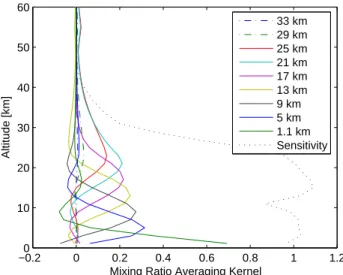
data has been evaluated for a typical measurement at Kiruna with a solar zenith angle of 70◦(F. Hase, private communi-cation). For N2O, the random error matrix is dominated by the contributions from the spectral baseline error, as well as the temperature profile uncertainties. For HNO3, the spec-tral noise is also a dominant error source. Figure 6 shows the square-root of the variances of Sx1 for the FTIR N2O and
HNO3retrievals at the Kiruna station.
The ESA MIPAS products include individual error covari-ance matrices with each profile: they represent the errors due to the noise. As only a typical value is used for the ground-based FTIR uncertainty, we have taken for the MIPAS error covariance matrix due to noise, Sn, the mean of the
matri-ces corresponding to all the MIPAS scans collocated within 1000 km around the stations. A very few scans, with particu-larly high error values (larger than two times the mean error), have been rejected from the statistics.
An analysis of the various other sources of error of the MI-PAS retrievals has been made by the Atmospheric, Oceanic and Planetary Physics (AOPP) research team at Oxford Uni-versity6. The systematic errors given by AOPP are typical ones for large latitude bands. These errors are given in per-cent in an altitude grid, and it is assumed that there are no correlations between errors, i.e., each systematic error co-variance matrix is diagonal. The systematic errors are di-vided into two parts: purely systematic errors and systematic errors with random variability. For the discussion about the scatter of the comparisons, we are interested only in the ran-dom error sources (noise and systematic errors with ranran-dom variability, namely: propagation of temperature random er-ror on the retrievals, horizontal gradient effects, uncertainties on the profiles of interfering species and on the high altitude column). Hereinafter, we will designate this random error by the short term “uncertainty”. The total error covariance matrix due to all systematic error sources with random vari-ability, Ssyst rand, has been calculated as the mean of the set of
0 10 20 30 40 50 0 10 20 30 40 50 60 70 vmr [ppbv] Altitude [km]
N2O random errors at Kiruna Random error FTIR
Random error MIPAS "smoothed" Random error of the difference MIPAS−FTIR
0 0.05 0.1 0.15 0.2 0.25 0.3 0.35 0.4 0.45 0 10 20 30 40 50 60 70 vmr [ppbv] Altitude [km] HNO
3 random errors at Kiruna Random error FTIR
Random error MIPAS "smoothed" Random error of the difference MIPAS−FTIR
Fig. 6. Ground-based FTIR, MIPAS and (MIPAS-FTIR) random errors (in ppbv) for the N2O and HNO3retrievals at Kiruna.
individual matrices in vmr units, obtained from the multipli-cation of the typical matrix in percentage with the individual MIPAS profile for each coincidence case.
Then the contribution of the MIPAS uncertainties to the combined random error covariance matrix Sδ12 in Eq. (2) is
simply: Sx2=Sn+Ssyst rand.
Figure 6 shows the square-root of the variances of the smoothed MIPAS profile uncertainty matrix (second term on the right hand of Eq. 2) for the N2O and HNO3 retrievals obtained around the Kiruna station, together with the square-root of the variances of Sx1 and Sδ12for the FTIR profile and
for the absolute difference MIPAS-FTIR, respectively. From the error covariance matrix of the difference MIPAS-FTIR, we have calculated the error 1δP C associated with the
difference of partial columns. This calculation is made ac-cording to:
1δP C =g
TS
δ12g, (5)
in which g is the operator that transforms the volume mixing ratio profile in a partial column amount, between the bound-aries that have been defined earlier (Sect. 3.3 and Table 2).
Since we discuss the results of the statistical evaluations in percentage values in the next section, we calculate the relative error on the partial column differences by dividing the absolute error (Eq. 5) by the mean of the FTIR partial columns. This relative random error on the difference be-tween MIPAS and FTIR partial columns is given in Tables 3, and 5, and will be compared to the standard deviations of the comparisons statistics to verify whether both instruments are in agreement. This is the subject of the next section.
6 Results of the intercomparisons
6.1 Results for N2O
6.1.1 Comparisons of the partial columns of N2O
Table 3 summarizes, for each station, the statistical results of the comparisons of the partial columns of N2O for the four sets described in Sect. 5.2. As seen in Sect. 2, the vertical coordinate for the comparisons must be pressure rather than altitude. The pressure limits of the partial columns are re-peated in the table.
Table 3 shows that there is a good agreement between MIPAS and ground-based FTIR partial columns even with the less constrained collocation criteria (“Statistics 1”). For Kiruna, Jungfraujoch and Lauder, there is no statistically sig-nificant bias between the two instruments considering the means and their error (about 2%, calculated as explained in Sect. 5.2) for “Statistics 1”. A small positive bias of 4±2% is obtained at Wollongong, and a negative one of −5±2% at Arrival Heights. The random errors of the relative differ-ences of partial columns, estimated as seen in Sect. 5.3.2, are about 6 or 7% as indicated in the table. Agreement be-tween both instruments should give a standard deviation of the statistics similar to the estimated random errors. One ex-pects that the remaining discrepancies of a few percent be-tween the two instruments are due to spatial collocation cri-teria that are too wide. “Statistics 2”, made with a reduced collocation criterion of 400 km, have indeed lower standard deviations for the three stations where the number of coinci-dences remains statistically relevant (≥10).
The reason why the standard deviation of the statistics is not reduced at the Kiruna station by using a stricter
collo-Table 3. Statistical means and standard deviations [<X-FTIR>±1σ ]/<FTIR> [%] of the N2O partial columns confined between the given pressure limits. X stands for the MIPAS partial columns collocated within 1000 km (“Statistics 1”) and 400 km (“Statistics 2”) around the ground-based stations, or, the BASCOE partial columns corresponding to cases where MIPAS data exist within the adopted collocation times (“Statistics 3”) and for all cases where FTIR ground-based data exist (“Statistics 4”). All X profiles have been smoothed by the ground-based FTIR averaging kernel matrices as explained in Sect. 5.1. The numbers of comparisons included in the different statistics are given between parentheses.
N2O [<MIPAS-FTIR>±1σ ]/<FTIR> [<BASCOE-FTIR>±1σ ]/<FTIR> Station Pressure “Statistics 1” “Statistics 2” Random “Statistics 3” “Statistics 4”
limits [hPa] [%] [%] errorα[%] [%] [%]
Kiruna (68◦N) 182–24 −1±9 (283) −4±9 (6) 6 +0±7 (86) +0±7 (119)
Jungfraujoch (46.5◦N) 198–1 +2±6 (130) +1±3 (10) 6 +0±2 (64) +0±2 (176)
Wollongong (34◦S) 207–12 +4±7 (78) +9±10 (4) 6 +0±3 (31) −1±3 (133)
Lauder (45◦S) 199–12 +0±7 (194) +4±5 (11) 6 +0±4 (89) +1±4 (273)
Arrival Heights (78◦S) 181–17 −5±10 (271) −8±9 (24) 7 −5±6 (48) −4±8 (70)
αSee Sect. 5.3.2 for the estimation of the error on the relative differences.
Table 4. Same as Table 3 but for a reduced (summer-autumn) time period, at Kiruna and Arrival Heights.
N2O [<MIPAS-FTIR>±1σ ]/<FTIR> [<BASCOE-FTIR>±1σ ]/<FTIR> Station Pressure “Statistics 1” “Statistics 2” Random “Statistics 3” “Statistics 4”
limits [hPa] [%] [%] error [%] [%] [%]
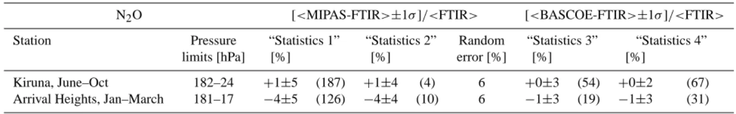
Kiruna, June–Oct 182–24 +1±5 (187) +1±4 (4) 6 +0±3 (54) +0±2 (67)
Arrival Heights, Jan–March 181–17 −4±5 (126) −4±4 (10) 6 −1±3 (19) −1±3 (31)
cation criteria can be understood from the timeseries of the partial columns of N2O in this particular case, as shown in Fig. 7. We see that the variation of the N2O abundances is much higher during the winter-spring period (January to end of March), probably related to subsidence in polar vor-tex conditions. Thus, the higher standard deviation of 9% at Kiruna for “Statistics 1” is due to the higher variability of N2O in time and space. This makes the collocation crite-rion less adequate for selecting comparable quantities. The standard deviation remains high (9%) even if the spatial col-location is set to 400 km. It is probably because in spring even a collocation of 400 km is not sufficient to take into ac-count the N2O spatial variability and because the horizontal smoothing error (see Sect. 5.3.1) is larger during this period. We can however not conclude because of the bad statistical conditions (only six coincidences, two of them occuring in spring). But a similar problem to Kiruna is encountered at the Arrival Heights station as seen in Fig. 8, with a high vari-ability of N2O in local spring (September to end of Novem-ber), thus giving rise to standard deviations of “Statistics 1” and “2” (10% and 9%, respectively) that are high compared to the random error of 6%. To confirm this interpretation, the statistics of the comparisons (relative differences between FTIR and MIPAS partial column values) at Kiruna and Ar-rival Heights, limited to the local summer-autumn period, are given in Table 4. They show values for the standard
devia-tions that are in agreement with the expected uncertainty for the relative differences, and that decrease from “Statistics 1” to “Statistics 2”.
At the Wollongong station, “Statistics 2” suffers from a very small number of coincidences, in which essentially one out of the four MIPAS scans in coincidence, in early March, is causing the large value of the standard deviation (10%). Eliminating this point reduces the bias and the standard de-viation to 4±3%.
As said before, for the purpose of evaluating the impact of the collocation criteria on the comparison results, we have also compared the FTIR data with correlative data from BASCOE analyses, i.e., BASCOE analyses interpolated at the location of the ground stations as proxies for perfectly collocated MIPAS measurements, in “Statistics 3” and “4”. A comparison in Table 3 of the results for “Statistics 1” to those for “Statistics 3”, which include identical sets of FTIR measurements, shows lower standard deviations in the latter case, especially for the three mid-latitudes stations. A simi-lar reduction in the standard deviations is observed in Table 4 for the two high latitude stations, Kiruna and Arrival Heights, when the reduced time period is considered. One also no-tices very small differences between the results (means and standard deviations) of “Statistics 3” and “Statistics 4” where BASCOE products are used even when there are no MIPAS observations that satisfy the temporal and spatial collocation
4 5 6 7 8 9 10x 10 17 PC amount [molec. cm −2 ]
Partial columns (182−24 hPa) of N
2O at Kiruna
FTIR
MIPAS < 1000 km MIPAS < 400 km BASCOE
Jan 03 Apr 03 Jul 03 Oct 03 Jan 04 −40 −20 0 20 40 Differences [%] Date
Fig. 7. Upper panel: Partial columns (182–24 hPa) of N2O at
Kiruna, from ground-based FTIR (green circles), MIPAS (dark blue and light blue stars for selections according to the spatial collocation criteria of 1000 and 400 km, respectively) and BASCOE (magenta triangles) data. Lower panel: Relative partial column differences (MIPAS-FTIR)/<FTIR> (stars; same colour coding as for upper plot), and (BASCOE-FTIR)/<FTIR> (magenta triangles).
criteria with the FTIR measurements. These results confirm that BASCOE products can be used reliably as proxies of MI-PAS observations at any time within the considered periods. Still, in the winter-spring periods at high latitudes, where the spatial (and temporal) variability of the N2O partial column abundances is high, it appears that BASCOE, with its res-olution of 5◦ in longitude and 3.75◦ in latitude, has more difficulties to correctly capture this variability: the standard deviations of “Statistics 3” or “4” do not go down to the level of the random uncertainty (except “Statistics 3” for Arrival Heights). This is in agreement with Fig. 5 which shows that the standard deviations of the statistics comparing BASCOE and MIPAS are larger for the months January to March at Kiruna, and September to November for Arrival Heights.
One may also notice that the comparisons of BASCOE and FTIR show a significant bias only for Arrival Heights, when the whole period January to December 2003 is considered.
From the best cases (mid-latitude stations) of Table 3 and from Table 4, we see that the statistical standard deviations of the observed partial column differences can be slightly smaller than the estimated random uncertainties associated
4 5 6 7 8 9 10x 10 17 PC amount [molec. cm −2 ]
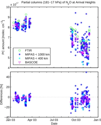
Partial columns (181−17 hPa) of N
2O at Arrival Heights
FTIR
MIPAS < 1000 km MIPAS < 400 km BASCOE
Jan 03 Apr 03 Jul 03 Oct 03 Jan 04 −40 −20 0 20 40 Differences [%] Date
Fig. 8. Upper panel: Partial columns (181–17 hPa) of N2O at
Arrival Heights, from ground-based FTIR (green circles), MIPAS (dark blue and light blue stars for selections according to the spatial collocation criteria of 1000 and 400 km, respectively) and BASCOE (magenta triangles) data. Lower panel: Relative partial column dif-ferences (MIPAS-FTIR)/<FTIR> (stars; same colour coding as for upper plot), and (BASCOE-FTIR)/<FTIR> (magenta triangles).
with them. This could lead to the conclusion that the uncer-tainty estimates for the FTIR profiles are conservative. How-ever, we’ll see in the profile comparisons in the next sec-tion that the ratio between the statistical standard deviasec-tion and the random error varies a lot with altitude (Fig. 9). The overestimation of the random error appears only in the tro-posphere and lower stratosphere where the amount of N2O is important.
6.1.2 Comparisons of the vertical profiles of N2O
Figure 9 shows the statistical means and associated stan-dard deviations of the relative differences between the ver-tical profiles of N2O from the ground-based FTIR observa-tions and MIPAS v4.61 (“Statistics 1”) and BASCOE prod-ucts (“Statistics 3”), at the five contributing stations. The ran-dom error on the difference between MIPAS and FTIR pro-files, i.e., the square-root of the variances of Sδ12(Eq. 2), are
represented by the shaded areas around the statistical means of the MIPAS-FTIR difference profiles. As we show rela-tive differences, the absolute errors have been divided by the mean of the FTIR profiles.
Table 5. Statistical means and standard deviations [<X-FTIR>±1σ ]/<FTIR> [%] of the HNO3partial columns confined between the given pressure limits. X stands for the MIPAS partial columns collocated within 1000 km (“Statistics 1”) and 400 km (“Statistics 2”) around the ground-based stations, or, the BASCOE partial columns corresponding to cases where MIPAS data exist within the adopted collocations times (”Statistics 3”) and for all cases where FTIR based data exist (“Statistics 4”). All X profiles have been smoothed by the ground-based FTIR averaging kernel matrices as explained in Sect. 5.1. The numbers of comparisons included in the different statistics are given between parentheses. K.: Kiruna; A.H.: Arrival Heights.
HNO3 [<MIPAS-FTIR>±1σ ]/<FTIR> [<BASCOE-FTIR>±1σ ]/<FTIR> Station Pressure “Statistics 1” “Statistics 2” Random “Statistics 3” “Statistics 4”
limits [hPa] [%] [%] error [%] [%] [%]
Kiruna 132–4 +12±12 (362) +20±7 (6) 3 +5±7 (91) +5±9 (126) K., June-Oct +13±9 (248) +18±6 (4) 3 +4±6 (61) +5±6 (74) Jungfraujoch 145–15 +16±17 (167) +14±12 (14) 4 +6±7 (60) +5±8 (165) Wollongong 151–9 +11±17 (62) +10±3 (2) 4 +12±10 (26) +10±9 (131) Lauder 144–7 +15±13 (132) +17±7 (9) 3 +4±8 (46) +2±9 (138) Arrival Heights 135–7 +19±23 (318) +17±14 (33) 3 +1±13 (51) +2±12 (68) A. H., Jan-March +20±9 (126) +19±5 (10) 3 +12±4 (19) +11±5 (28)
The black horizontal bars in Fig. 9 indicate the pressure limits of the partial columns defined in Table 3. As stated before, the MIPAS profiles are extrapolated with the MI-PAS initial guess (IG2) values outside the vertical ranges of the measurements. The ground-based FTIR profiles and the smoothed MIPAS profiles tend towards the a priori profiles at altitudes where the sensitivity of the retrievals to the mea-surements tends to zero. This explains why the relative dif-ference profiles and associated errors all tend to zero at high altitudes.
For Kiruna, we see in Fig. 9 a positive bias (below 3%) between MIPAS and FTIR at low altitudes becoming nega-tive (below 5%) for pressure smaller than 100 hPa. This be-haviour is similar for both whole and reduced periods. Con-sidering the error on the mean of the differences (not plotted here, but calculated as discussed in Sect. 5), this bias is statis-tically significant only for pressure smaller than 80 hPa. The same kind of shape is seen at Lauder, the higher positive bias at low altitude (below 4%) being also statistically significant. At Jungfraujoch, the bias is positive (below 4%) for pressure greater than 40 hPa and become negative above (below 5%, for pressure greater than 20 hPa; below 10% above). At Wol-longong, a high positive bias is observed (below 5% for pres-sure greater than 55 hPa with a maximum of 21% at 25 hPa). At Arrival Heights a negative significant bias is seen for the whole altitude range, below 8% and 5% for the whole and reduced period, respectively. The shape of the bias look very similar for both compared data sets, MIPAS and BASCOE. This confirms that for the purpose of the present comparison, the agreement between MIPAS and BASCOE N2O, as seen in Fig. 5, allows the assimilated dataset to be a proxy of the satellite observations, with continuous coverage in space and time. This shows also that the biases between each dataset and the FTIR observations is probably not related to colloca-tion issues, but rather to the shapes of the FTIR retrievals. As
the DOFS for the FTIR N2O retrievals between the consid-ered pressure limits is between 1.3 and 2.7 (for Kiruna and Jungfraujoch, respectively; see Table 2), the detailed shape of the FTIR profiles strongly depends on the retrieval settings.
As seen with the partial columns comparisons in Table 3, the standard deviations of the relative differences are reduced when using collocated BASCOE products instead of the cor-relative MIPAS data. When comparing the random error and the statistical standard deviations, one should consider that the error calculation has been made using a typical case at Kiruna where the sensitivity is below 0.5 for altitudes greater than 25 km (Table 2). We observe that the statistical stan-dard deviations are lower than the estimated random error for pressures greater than 100 hPa (around 15.5 km), in the troposphere and low stratosphere, where the N2O amount is important.
6.2 Results for HNO3
6.2.1 Comparisons of the partial columns of HNO3 Analogous to the presentation for N2O in Table 3, Table 5 gives the statistical results, at each station, for the compar-isons between FTIR and MIPAS or BASCOE HNO3partial column values, according to the four statistical approaches described in Sect. 5.2. The partial column limits (in pressure units) are also included in the second column of Table 5.
The first striking observation is that there exists a negative bias between the FTIR and MIPAS data, of order 11 to 19%. A negative bias is expected and has been observed in previ-ous validation work (Oelhaf et al., 2004). It is due to a scal-ing factor that was applied to the HNO3line intensities in the spectroscopic database used for the MIPAS v4.61 retrievals, mipas−pf3.1 (Flaud et al., 2003a,b; Raspollini et al., 2006),
as compared to the databases used for the ground-based FTIR retrievals (HITRAN 2000, see Sect. 3.2.1). It is well-known
−50 −40 −30 −20 −10 0 10 20 30 40 50 100 101 102 103 [%] Pressure [hPa] N2O at Kiruna −50 −40 −30 −20 −10 0 10 20 30 40 50 45.5 30.5 15.5 0.0 Approximate altitude [km]
[<MIPAS − FTIR> ± 1σ] / <FTIR>
[<BASCOE − FTIR> ± 1σ] / <FTIR>
Random error on the differences (MIPAS − FTIR)
−50 −40 −30 −20 −10 0 10 20 30 40 50 100 101 102 103 [%] Pressure [hPa]
N2O at Kiruna during the reduced period Jun−Oct 2003
−50 −40 −30 −20 −10 0 10 20 30 40 50 45.5 30.5 15.5 0.00 Approximate altitude [km] −50 −40 −30 −20 −10 0 10 20 30 40 50 100 101 102 103 [%] Pressure [hPa] N2O at Jungfraujoch −50 −40 −30 −20 −10 0 10 20 30 40 50 46.5 30.2 15.8 0.2 Approximate altitude [km] −50 −40 −30 −20 −10 0 10 20 30 40 50 100 101 102 103 [%] Pressure [hPa] N2O at Wollongong −50 −40 −30 −20 −10 0 10 20 30 40 50 48.5 31.2 16.5 0.2 Approximate altitude [km] −50 −40 −30 −20 −10 0 10 20 30 40 50 100 101 102 103 [%] Pressure [hPa] N2O at Lauder −50 −40 −30 −20 −10 0 10 20 30 40 50 48.9 31.4 16.3 0.2 Approximate altitude [km] −50 −40 −30 −20 −10 0 10 20 30 40 50 100 101 102 103 [%] Pressure [hPa] N2O at Arrival Heights −50 −40 −30 −20 −10 0 10 20 30 40 50 50.2 31.9 16.0 0.0 Approximate altitude [km] −50 −40 −30 −20 −10 0 10 20 30 40 50 100 101 102 103 [%] Pressure [hPa]
N2O at Arrival Heights during the reduced period Jan−Mar 2003
−50 −40 −30 −20 −10 0 10 20 30 40 50 50.2 31.9 16.0 0.0 Approximate altitude [km]
Fig. 9. Statistical means and standard deviations [<X-FTIR>±1σ ]/<FTIR> [%] of the N2O difference profiles. X represents the MIPAS
collocated scans within 1000 km around the stations (“Statistics 1”, in blue) or the BASCOE correlative profiles (“Statistics 3”, in magenta). All X profiles have been smoothed by the ground-based FTIR averaging kernel matrices as discussed in Sect. 5.1. The numbers of coin-cidences included in both comparison data sets are given in Table 3. The black horizontal bars indicate the pressure limits of the partial columns defined before (see also Table 3). The shaded area represents the random uncertainty on the differences, in % (see Sect. 5.3.2).
0 0.5 1 1.5 2 2.5x 10 16 PC amount [molec. cm −2 ]
Partial columns (135−7 hPa) of HNO
3 at Arrival Heights
FTIR
MIPAS < 1000 km MIPAS < 400 km BASCOE
Jan 03 Apr 03 Jul 03 Oct 03 Jan 04 −50 0 50 100 Differences [%] Date
Fig. 10. Upper panel: Partial columns (135–7 hPa) of HNO3at
Arrival Heights, from ground-based FTIR (green circles), MIPAS (dark blue and light blue stars for selections according to the spatial collocation criteria of 1000 and 400 km, respectively) and BASCOE (magenta triangles) data. Lower panel: Relative partial column dif-ferences (MIPAS-FTIR)/<FTIR> (stars; same colour coding as for upper plot), and (BASCOE-FTIR)/<FTIR> (magenta triangles).
that the difference in the HNO3 spectroscopic parameters between HITRAN 2000 and mipas−pf3.1 induces a bias of
about 14% between the retrieved vmr profiles (Raspollini et al., 2006). The determination of accurate HNO3line inten-sities is still controversial and in progress (see Flaud et al. (2006) and the references therein). If the same spectroscopy would have been adopted for the MIPAS and FTIR retrievals, the biases would have been 14% smaller, and thus would not have been statistically significant except for Arrival Heights. At the latter station, a mean positive bias of 5% would still be significant compared to the error on the mean of 4%.
In the case of HNO3, the use of BASCOE analyses as proxies for the MIPAS data appears to be more problematic when one is looking at absolute concentration values. The comparisons between BASCOE and FTIR do not show the systematic bias that is observed in the direct MIPAS-FTIR comparisons, except at Wollongong. The bias between BAS-COE assimilation analyses for HNO3and the MIPAS HNO3 data, discussed in Sect. 4 and shown in Fig. 5, is clearly seen in Figs. 10 and 11. Even if the products of BASCOE seem to be closer to the ground-based FTIR products, it is not
pos-0.6 0.8 1 1.2 1.4 1.6 1.8x 10 16 PC amount [molec. cm −2 ]
Partial columns (145−15 hPa) of HNO
3 at Jungfraujoch
FTIR
MIPAS < 1000 km MIPAS < 400 km BASCOE
Jan 03 Apr 03 Jul 03 Oct 03 Jan 04 −40 −20 0 20 40 60 Differences [%] Date
Fig. 11. Upper panel: Partial columns (145–15 hPa) of HNO3at
the Jungfraujoch, from ground-based FTIR (green circles), MIPAS (dark blue and light blue stars for selections according to the spatial collocation criteria of 1000 and 400 km, respectively) and BASCOE (magenta triangles) data. Lower panel: Relative partial column dif-ferences (MIPAS-FTIR)/<FTIR> (stars; same colour coding as for upper plot), and (BASCOE-FTIR)/<FTIR> (magenta triangles).
sible to conclude that the MIPAS measurements of HNO3 are too high. Still, BASCOE nicely reproduces the seasonal variation.
The second noticeable fact in Table 5 is that the standard deviations of all statistics are significantly larger than ex-pected on the basis of the random uncertainties of the rel-ative partial column differences which are only 3 or 4%. If the same spectroscopy had been adopted for the MIPAS and FTIR retrievals, the standard deviation would have decreased by a factor of 0.86. This would give, for “Statistics 4”, a stan-dard deviation of 4% in the best case of Arrival Heights lim-ited to the January-March period, up to 10% in the worst case of Arrival Heights when the whole year 2003 is considered. This means that the additional coincidence and horizontal smoothing errors described in Sect. 5.3.1 are significant in the comparisons between the FTIR and MIPAS products. In-deed, the additional uncertainties can largely be explained by the spatial variability of HNO3. It is clearly seen in Table 5 by comparing “Statistics 1” and “2”, that a stricter colloca-tion criterion reduces the standard deviacolloca-tions significantly. One could expect that the use of BASCOE would reduce the standard deviations to the level of the estimated random
un-−100 −80 −60 −40 −20 0 20 40 60 80 100 100 101 102 103 [%] Pressure [hPa] HNO3 at Kiruna 45.5 30.4 15.5 0.0 Approximate altitude [km]
[<MIPAS − FTIR> ± 1σ] / <FTIR>
[<BASCOE − FTIR> ± 1σ] / <FTIR>
Random error on the differences (MIPAS − FTIR)
−100 −80 −60 −40 −20 0 20 40 60 80 100 100 101 102 103 [%] Pressure [hPa]
HNO3 at Kiruna during the reduced period Jun−Oct 2003
45.5 30.4 15.5 0.0 Approximate altitude [km] −100 −80 −60 −40 −20 0 20 40 60 80 100 100 101 102 103 [%] Pressure [hPa] HNO3 at Jungfraujoch 46.4 30.2 15.8 0.2 Approximate altitude [km] −100 −80 −60 −40 −20 0 20 40 60 80 100 100 101 102 103 [%] Pressure [hPa] HNO3 at Wollongong 48.5 31.2 16.5 0.2 Approximate altitude [km] −100 −80 −60 −40 −20 0 20 40 60 80 100 100 101 102 103 [%] Pressure [hPa] HNO3 at Lauder 48.9 31.4 16.3 0.1 Approximate altitude [km] −100 −80 −60 −40 −20 0 20 40 60 80 100 100 101 102 103 [%] Pressure [hPa]
HNO3 at Arrival Heights
50.2 31.9 16.0 0.0 Approximate altitude [km] −100 −80 −60 −40 −20 0 20 40 60 80 100 100 101 102 103 [%] Pressure [hPa]
HNO3 at Arrival Heights during the reduced period Jan−Mar 2003
50.2
31.9
16.0
0.0
Approximate altitude [km]
Fig. 12. Statistical means and standard deviations [<X-FTIR>±1σ ]/<FTIR> [%] of the HNO3difference profiles. X represents the
MIPAS collocated scans within 1000 km around the stations (“Statistics 1”, in blue) or the BASCOE correlative profiles (“Statistics 3”, in magenta). All X profiles have been smoothed by the ground-based FTIR averaging kernel matrices as discussed in Sect. 5.1. The numbers of coincidences included in both comparison data sets are given in columns 1 and 3 of Table 5. The black horizontal bars indicate the pressure limits of the partial columns defined before (see also Table 5). The shaded area represents the random uncertainty on the differences, in % (see Sect. 5.3.2).


![Table 5. Statistical means and standard deviations [ <X-FTIR> ± 1σ ] /<FTIR> [%] of the HNO 3 partial columns confined between the given pressure limits](https://thumb-eu.123doks.com/thumbv2/123doknet/6289058.164570/14.892.98.797.214.403/table-statistical-standard-deviations-partial-columns-confined-pressure.webp)
