Self-heating of bulk high temperature superconductors of finite height subjected to a large alternating magnetic field

Self-heating of bulk high temperature superconductors

of finite height subjected to a large alternating magnetic field

P Laurent1_{, J-F Fagnard}2_{, N Hari Babu}3_{, D A Cardwell}4_{, B Vanderheyden}1 _{and P}

Vanderbemden1

(1) SUPRATECS and Department of Electrical Engineering and Computer Science B28, Sart-Tilman, B-4000 Liège, Belgium

(2) SUPRATECS, Royal Military Academy of Belgium, Avenue de la Renaissance, B-1000 Brussels, Belgium

(3) Brunel Centre for Advanced Solidification Technology (BCAST), Brunel University, West London, UB8 3PH, UK

(4) Bulk Superconductivity Group, Engineering Department, University of Cambridge, Cambridge, CB2 1PZ, UK

E-mail : Philippe.Vanderbemden@ulg.ac.be

Abstract. In this work we study, both experimentally and numerically, the self-heating of a

bulk, large YBCO pellet of aspect ratio (thickness / diameter) ~ 0.4 subjected to a large AC magnetic field. To ensure accurate temperature measurements, the sample was placed in an experimental vacuum chamber to achieve a small and reproducible heat transfer coefficient between the superconductor and the cryogenic fluid. The temperature was measured at several locations on the sample surface during the self-heating process. The experimentally determined temperature gradients are found to be very small in this arrangement (< 0.2 K across the radius of the superconductor). The time-dependence of the average temperature T(t) is found to agree well with a theoretical prediction based on the one-dimensional (1-D) Bean model, assuming a uniform temperature in the sample. A 2-D magneto-thermal model was also used to determine the space and time-dependent temperature distribution T(r, z, t) during the application of the AC field. The losses in the bulk pellet were determined using an algorithm based on the numerical method of Brandt, which was combined with a heat diffusion algorithm implemented using a finite-difference method. The model is shown to be able to reproduce the main trends of the observed temperature evolution of the bulk sample during a self-heating process. Finally, the 2-D model is used to study the effect of a non-uniform distribution of critical current density Jc(r, z) on the losses within the bulk superconductor.

1. Introduction

Bulk melt-processed Y-Ba-Cu-O (YBCO), high temperature superconductors (HTS) are usually fabricated in disc or cylindrical geometries for various permanent magnet-like applications [1,2], such as rotating machines [3-6] or magnetic bearings [7-10], due to their ability to trap large magnetic inductions [11-14]. In some applications, however, the bulk superconductor may experience periodic variations of the applied magnetic field that are caused, for example, by vibrations or irregular magnetization by a permanent magnet interacting with the sample [15,16]. The resulting hysteresis losses caused by the associated vortex motion may induce a temperature increase of the superconductor [17,18], which, in turn, reduces the critical current density and has a detrimental effect on the flux trapped in the material [19-28].

Thermal effects arising in a bulk superconductor subjected to a variable magnetic field H(t) have been studied in the literature for various time-dependences of H(t), including AC fields [22-29], which are also considered in the present work. The self-heating of the sample is determined by both the AC losses and the thermal exchange between the superconductor and the cryogenic coolant [30, 31]. In the present study, we extend our previous work [29] in which parameters affecting the self-heating were determined analytically using a one-dimensional (1-D) model. We consider a cylindrical sample (figure 1), cooled initially to temperature T0 before being subjected to an AC magnetic field H(t) = Hm sin(ωt), applied at t = 0. At low field amplitude Hm, the sample temperature increases and reaches a steady-state value that is function of Hm but much lower than the superconducting critical temperature Tc. Thermal runaway occurs at high field amplitudes, on the other hand, which results in a sharp increase in temperature up to an equilibrium value that is close to (but slightly smaller than) Tc. The simplest way to address this problem is to assume that the sample temperature T is uniform, i.e. to neglect thermal gradients within the sample during the heating process. This approach was used by Tsukamoto et al. [22], Zushi et al. [23,24] who were able subsequently to model successfully the self-heating behaviour under AC magnetic fields by adopting a relatively simple 1-D Bean analysis [32]. In our recent work [29], we derived analytical expressions for the sample equilibrium temperature and were able to show that the threshold magnetic field Htr2 (separating the two regimes corresponding to a final temperature being either much smaller or close to Tc) is given approximately by;

(

)

where A is the contact area between the sample and the coolant, U is the convective heat transfer coefficient, Tc is the superconducting critical temperature, T0 is the coolant temperature, Jc0 is the critical current density at the coolant temperature, a is the radius of the cylinder, µ0 is the magnetic

permeability of free space, f is the frequency of the applied field and V is the sample volume.

The magneto-thermal analysis referred to above assumes a uniform sample temperature T. This approach is justified if the heat diffusion rate across the sample is faster than the rate of exchange with the cryogenic environment or, in other words, if the thermal conductivity of the superconductor, κ, is much higher than the (U a) product, in such a way that the dimensionless Biot number Bi = U a / κ is much smaller than unity [28]. In our experimental system, which was designed for simultaneous thermal and magnetic measurements [33], the sample is placed in an experimental chamber and exposed to a medium vacuum (pressure ~ 10-2 – 10-1 mbar). As a result, the convective coefficient U is low and the Biot number is estimated to be ~ 0.02 [29]. Such a low value suggests that the temperature distribution within the sample is effectively uniform, although it is likely that the AC magnetic field penetrates a thin layer close to the sample surface. In practice, however, thermal gradients are almost certainly present within the superconductor. It is of interest, therefore, to determine experimentally the amplitude of such thermal gradients, the location of the warmest points, and to investigate whether the observed behaviour can be understood with a model taking into account the radial and axial temperature distributions T(r,z) in a cylinder of finite height subjected to an axial AC field.

These thermal aspects of a bulk superconductor exposed to a varying magnetic field will be investigated in the present paper, which is organized as follows. In Section 2, we present the two-dimensional magneto-thermal algorithm. Section 3 describes the experimental system used to achieve precise temperature measurements at several locations on a bulk melt-processed sample during the application of the AC field. Experimental data are presented and analyzed in Section 4, together with a model of the distribution of losses in the sample, characterized either by a uniform Jc or a non-uniform Jc(r,z). The conclusions are drawn in Section 5.

2. Model

2.1. Distribution of AC losses at a constant temperature

In order to study the penetration of the AC magnetic field in a superconducting cylinder of finite height, we use a semi-analytical approach based on the Brandt algorithm [34,35]. The method is based on the discretization and numerical integration of the Biot-Savart equations in order to determine the current density J(r, z, t) inside the volume of the superconductor [34-37]. We consider the geometry represented in the inset of figure 1, and follow the procedure described comprehensively in ref. [34]. Under an applied magnetic field varying gradually along the z direction, the induced electric field E, current density J and magnetic induction B assume the form, J = - J(r, z) eϕ , E = - E(r, z) eϕ, B = Br(r, z) er + Bz(r, z) ez, where er, ez and eϕ are the unit vector in the radial, axial and azimuthal directions

respectively. These parameters satisfy the following Maxwell equations;

curl E = - B& (2)

curl B = µ0 J (3)

where the constitutive law B = μ0H is assumed. In order to avoid the computation of the magnetic

induction B in the infinite region exterior to the sample, an equation is established for the time evolution of the macroscopic current density J as a function of the electric field in the volume of the superconductor. This equation takes the form [34]:

J& (r, r’, t) =

∫

∫

Q-1(r, z, r’, z’) { E[J(r, r’, t)] – r &Bapp

2 (t)} (4)

where Bapp(t) denotes the applied induction Bapp(t) = µ0Hm sin(ωt) and Q(r, z, r’, z’) is a geometry-dependent integral kernel which can be evaluated numerically [34]. The current density J can then be obtained by discretizing and integrating numerically Eq. (4), in which E is eliminated using the classical constitutive law;

n c c J J E E _⎟⎟ ⎠ ⎞ ⎜⎜ ⎝ ⎛ ⋅ = (5)

The model always assumes a field-independent Jc for simplicity. The exponent n is set to 25, which lies within the range of experimental values for melt-textured YBCO at 77 K and B < 1 T [38,39]. n is assumed to be constant in order to limit the number of variable modeling parameters. A field dependence n(B), however, can be introduced to the model, as considered, for example, in ref. [40-42]. Once the J(r, z, t) and E(r, z ,t) distributions are known, the local power averaged over one cycle, Pave(r, z), is given by;

(

) (

)

∫

2.2. Temperature distribution during self-heating

The Brandt algorithm described above is coupled to a heat diffusion algorithm enabling the temperature distribution of the sample T(r, z, t) to be computed with the finite-difference method. The temperature of the superconductor is assumed to be that of the cryogenic fluid T0, before being subjected to an axial AC magnetic field. The intrinsic Jc is assumed to be uniform throughout the sample. The power dissipated in the superconductor Pave(r, z) produces an inhomogeneous temperature distribution T(r, z) that translates into a inhomogeneous critical current density distribution Jc[T(r, z)] due to the temperature-dependence of Jc. The main algorithm is based on two sub-programs:

(i) the Brandt algorithm is used to compute, for one period of the AC field, the power dissipated locally P(r, z) for a given Jc(r, z) distribution for a constant temperature;

(ii) the “heat diffusion” algorithm is used to compute the time-evolution of the local temperature T(r, z), for a given time interval ΔtH, caused by a given P(r, z) distribution and particular thermal boundary conditions. The local dissipated power is assumed to be constant during the calculation.

The “heat diffusion” algorithm is implemented as follows. First, the superconducting cylinder of finite height is discretized with steps Δr and Δz, i.e. the sample is sub-divided into Nr × Nz rings of width Δr and thickness Δz, as illustrated schematically in figure 2. The symmetry of the geometry means that we can study the upper half of an axisymmetric system. A constant convective heat transfer coefficient U is set for the top surface (z = b) and the lateral surface (r = a). Note that since the bulk sample is in medium vacuum, heat transfer processes occur through conduction in the low pressure gas surrounding the sample, conduction in the chamber walls and radiation. The U value is therefore an overall heat transfer coefficient taking into account all barriers to heat transfer between the sample and the coolant. Figure 2(b) shows the cross-section of a ring of thickness Δz and width Δr. No heat flux flows parallel to the cylinder axis [Qin(0, z) = 0] or through the central plane [Qdown(r, 0) = 0]. The time-evolution of the ring temperature can be calculated from the distribution of the dissipated power P(r, z), as follows: V ) z , r ( P Q t T c V i i p _Δ Δ Δ Δ ⋅ = + ⋅ ⋅ ρ

∑

whereΔT is the finite variation of temperature during the finite time interval Δt. The Σ symbol indicates that the four heat fluxes Qup, Qdown, Qin and Qex shown in figure 2 are taken into account; they are calculated from the temperature of the neighbouring rings using the Fourier law [43]. Each ring element is characterized by a thermal conductivity κ, a specific heat cp, a density ρ and has a finite volume ΔV.

In the present case, the time interval ΔtH between two successive determinations of the temperature distribution is of the order of ~ 0.2 s. This time interval corresponds typically to 10-20 periods of the applied AC field. The critical current density is changed accordingly once the new temperature distribution is calculated. We assume a linear Jc(T) in our analysis, [22], although more refined models can also be used [44]. The Jc(T) law is given by;

( )

3. Experiment

Bulk melt-processed single domains of YBCO, consisting of a superconducting YBa2Cu3O7-δ (Y-123)

matrix with discrete Y2BaCuO5 (Y-211) inclusions, were fabricated by top seeded melt growth

(TSMG), as described in ref. [45]. The present study focuses on a single grain sample consisting of a single domain pellet of diameter 2a = 30 mm and thickness 2b = 12 mm, with an aspect ratio (b/a) of 0.4. The material is characterized by a critical temperature Tc ~ 91.6 K and a critical current density Jc of ~ 10

3

A/cm² at 77.4 K. For the modeling discussed below we choose a value of Jc = 1.2 × 103 A/cm². Note that such a value is below the average level that can be obtained for YBCO single domains fabricated using the top-seeded melt-growth technique. A sample of medium quality, but with uniform superconducting properties, was selected specifically for the magneto-thermal measurements reported here in order to ensure that the penetration depth of magnetic flux is not too small compared to the sample radius, and that sufficient losses will be generated within the sample at 77.4 K for experimentally accessible values of the applied magnetic field amplitude.

Magneto-thermal measurements on this YBCO sample were carried out using a bespoke AC susceptometer designed for the characterization of large superconducting samples (up to 32 mm diameter), as detailed in Ref. [33]. The sample is placed in a cylindrical experimental chamber made of ultra-high molecular weight polyethylene (PE-UHMW) of 5 mm thickness, as illustrated schematically in figure 2(c). The experimental chamber is immersed in liquid nitrogen. The sample space is connected to a vacuum rotary pump, enabling a medium vacuum (2 × 10-2 mbar at room temperature) to be achieved. This vacuum is maintained during the whole experiment. Four aluminized Plexiglas radiation shields are located between the top cap of the sample chamber and the sample in order to minimize radiation heating towards its top surface. In order to achieve the highest possible thermal insulation between the sample bottom surface and the bottom of the sample chamber, the sample is placed on an alumina plate supported by three small glass balls (2.4 mm in diameter) located at the vertices of a triangle, thereby producing in a very weak thermal link. Since the heat fluxes from the top and bottom surfaces of the sample are very small, the heat exchanged between the superconductor and the liquid nitrogen occurs mainly through the lateral face of the superconductor. This was checked using a computer modeling of the heat transfer rate between the sample and the experimental chamber of the susceptometer using the Engineering Equation Solver (EES ®) [46]. This configuration ensures a small, but reproducible, heat flux rate out of the sample. The convective heat transfer coefficient was determined to be U = 1.94 W/m²K [29], which is 3-4 orders of magnitude lower than the typical values of the pool boiling heat transfer coefficient from YBCO to liquid nitrogen [44,47]. The evolution of the sample temperature with time is monitored continuously during the application of the AC field using three type-E thermocouples (chromel-constantan) attached to the top surface at various locations from the centre.

4. Results and discussion

4.1. Distribution of ac losses at a constant temperature – modeling

First we investigate the distribution of AC losses in a short type-II superconducting cylinder, modeled numerically using the Brandt approach described in Section 2.1. The losses are averaged over one cycle of the AC field and are expressed in dimensionless units, which involves setting four parameters to unity: the magnetic permeability µ0, the critical current density Jc, the radius of the superconductor a, and the angular frequency ω. The specific losses expressed in SI units (i.e. [W/m³]) can be obtained by multiplying the dimensionless losses by the factor (ω µ0 Jc² a²).

Figure 3 shows the distribution of AC losses in a short cylindrical superconductor of aspect ratio (b/a) = 0.4 subjected to an axial AC magnetic field of amplitude H0 equal to half the full-penetration field, i.e. H0 = ½ Hp. The critical current density Jc is uniform throughout the sample. It can be seen that the losses are found to be maximum at the “corner” of the sample cross-section (r = a, z = b), which corresponds to the perimeter of the top and bottom cylindrical faces. The variation of the losses along the height of the cylindrical sample is found to be relatively small: the dissipated power within

the top face (z = b) is close to the power within the central plane (z = 0). In order to validate the results given by the two-dimensional (2-D) model, the losses are also calculated in the central plane of a “long” cylindrical superconductor of aspect ratio (b/a) = 3 and data are compared to the theoretical prediction from the 1-D Bean model. The inset of figure 3 compares the radial distribution of the dimensionless losses P(r) along the central plane of a long superconductor, calculated by the 2-D algorithm, with those predicted for an infinitely long cylinder, using a 1-D calculation [17]. In the 2-D algorithm 15 × 45 elements are used to calculate the current distribution. Although the number of elements (15) over the radius is relatively small, the results displayed in the inset of figure 3 show that the 1-D and the 2-D methods are in agreement. The maximum values of the normalised losses given by the 2-D model (0.0630) are slightly low compared to the 1-D prediction (0.0657). Note that the full-penetration field Hp for the long sample (2-D) is slightly smaller (98.2%) than that for the infinite cylinder, as can be calculated from the analytical expression for a finite cylinder [48]. However, the modeling is always carried out for field amplitude Hm = ½ Hp.

We now investigate the distribution of the losses when the distribution of superconducting properties is non-uniform over the cylinder radius and/or height. Such a situation is often encountered in bulk melt-textured (RE)BCO samples and may be attributed to several factors, including differences in the microstructure with increasing distance from the single crystal seed used for melt-processing [49], inhomogeneous distribution of pinning centres or differences in local oxygen stoichiometry within the bulk microstructure [50]. For simplicity, the Jc(r, z) dependence is always assumed to be linear. We consider six hypothetical distributions of the critical current density that give rise to the same average value of Jc (= 1 in dimensionless units). All distributions are assumed to have maximum and minimum values 1.5 and 0.5, as follows.

(a): Jc(0, z) = 0.5; Jc(a, z) = 1.5 (b): Jc(0, z) = 1.5; Jc(a, z) = 0.5 (c): Jc(r, 0) = 0.5; Jc(r, b) = 1.5 (d): Jc(r, 0) = 1.5; Jc(r, b) = 0.5 (e): Jc(0, 0) = 0.5; Jc(a, b) = 1.5; Jc(a, 0) = Jc(0, b) = 1 (f): Jc(0, 0) = 1.5; Jc(a, b) = 0.5; Jc(a, 0) = Jc(0, b) = 1

The results are summarized in figure 4. Compared to the “uniform Jc” case (figure 3), the losses are found to increase in the regions of the sample where Jc is the largest and to decrease in the regions where Jc is the smallest. The maximum value of the power dissipated occurs along the perimeter of the top and bottom surfaces [(r, z) = (a, b)], i.e. where the magnetic flux density is the largest, except when the Jc(a, b) = 0.5. The situation is particularly critical for the Jc distributions corresponding to Jc(a, b) = 1.5, i.e. for largest Jc along the perimeter of the bottom and top surfaces of the sample.

These results may be understood qualitatively by considering that the local losses are due to currents that flow along circumferential paths enclosing a time-dependent magnetic flux, the latter giving rise, according to Faraday’s law, to an azimuthal electric field. The average critical current density <Jc> in the region penetrated by vortices is the highest for critical current distributions corresponding to the highest Jc’s near the sample edges (e.g. situations (a), (c), and (e) in figure 4), since the AC field is chosen here smaller than the full-penetration field. In such cases, the volume of the region penetrated by moving vortices is globally smaller than for a uniform Jc, although the critical current density in these regions is high. This dominates and gives rise to globally higher losses in regions where the Jc is the highest, as observed in figure 4.

4.2. Temperature distribution during self-heating – experiment and modeling

We now consider the self-heating of the bulk YBCO cylindrical sample described in Section 3. The sample was placed in the experimental chamber of the susceptometer, cooled initially to the boiling point of liquid nitrogen, and then subjected to AC magnetic field H(t) = Hm sin(ωt) at t = 0. Magnetic field of amplitude and frequency µ0Hm = 34 mT and f = 91 Hz was then applied to the sample. The temperature was determined during the self-heating process at three locations on the sample top

surface: (i) at the “corner” location, (ii) at the centre, and (iii) between these two locations, as shown schematically in the inset of figure 5(a). We present here the results of the experiment and the model.

Figure 5(a) shows the time-dependence T(t) of the temperature measured on the top surface of the sample by the three thermocouples: edge [red], intermediate [blue] and centre [green]. First we note that the starting temperature of the experiment is 77.85 K, i.e. slightly greater than the theoretical temperature of pure liquid nitrogen at atmospheric pressure (77.4 K). The difference may be due to oxygen diffusion within the liquid nitrogen bath [51] and will not be considered further. For t < 500 s, the temperatures exhibit a sub-linear behaviour, followed by a change in concavity (t ≈ 520 s) just before the steady state is reached, at t ≈ 570 s. The average equilibrium temperature is equal to 91 K. When the steady-state is reached, the temperature of the central thermocouple is ~ 0.2 K higher than the temperature of the edge. Figure 6(a) shows an enlargement of the figure during the initial stage of the self-heating phenomena. It can be seen that the temperature rises first at the sample corner (red curve), although the temperatures recorded by the three thermocouples are very close to each other. The maximum temperature difference during the self-heating process measured on the top surface is ~ 0.1 K. Note also that the temperature increase starts as soon as the AC field is applied, which demonstrates the importance of using thermal sensors characterised by a small response time.

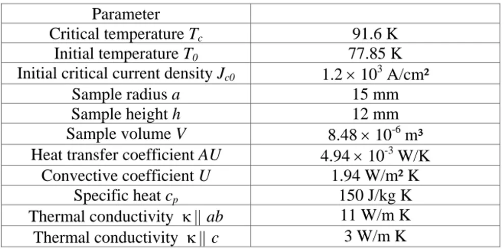
The small thermal gradient observed across the sample is consistent with the small value of the Biot number in the present experiment (Bi ~ 0.02). It is of interest to compare the experimental data to the theoretical predictions assuming a uniform sample temperature and infinite cylindrical geometry. The experimental parameters used in the calculations are summarized in table 1. From Eq. (1), the threshold field µ0Htr2 is estimated to 15.9 mT. The amplitude of the AC field (34 mT) is approximately twice the threshold field, and the expected theoretical behaviour (steady-state temperature close to Tc) is also observed experimentally in figure 5(a). More precisely, the theoretical final temperature Tsup is given by [29]:

(

)

i.e. Tsup ≈ 91.4 K, which is in reasonable agreement with the average equilibrium temperature observed experimentally (91 K). The most likely reason for the discrepancy is that the critical current density is assumed to be uniform and linearly temperature dependent in our model. Close to Tc, however, some deviations can be expected, essentially because of the inevitable distribution of Tc in the bulk sample that is due, for example, to small stoechiometry variations linked to the contamination by the seed single crystal. The average sample temperature T(t), assuming a linear Jc(T), can be obtained from the time-integration of the following equation [22]:

( )

( )

with the initial condition T(t=0) = T0. Using parameters listed in table 1, the theoretical T(t) can be obtained and is plotted in figure 5(b). Qualitatively, the theoretical average temperature agrees well with the experimental T(t) curves. The quantitative agreement is generally good, despite that the assumption of an infinite cylindrical geometry. This can be related to the modeled distribution of the losses shown in figure 3: the dissipated power is not found to depend strongly on the vertical coordinate (z), and, hence, finite size effects do not appear to play a crucial role. Furthermore, this simple model assumes a field-independent critical current density. The corresponding parameter Jc0, estimated from a Hall probe mapping measurement [52], invariably contains a degree of uncertainty because of (i) the finite distance between the probe and the sample surface and (ii) the difference between the trapped flux distribution above the top surface and that in the central plane [53,54]. Unlike the analytical expression of Htr2 [Eq. (1)] which is weakly influenced by an uncertainty on Jc0 (due to the “1/3” exponent), the precise Jc0 value affects directly the transient self-heating behaviour.

As an example, the initial slope of the T(t) curve can be calculated analytically for Hm << (Jc0 a), as follows:

( )

Hence the error in the parameter Jc0 produces the same error in the modeled initial value of temperature slope dT/dt.

Finally, we use the 2-D magneto-thermal algorithm to model the temperature distribution of the bulk sample during self-heating. The result is shown in figure 6(c) for 4 particular locations: 3 located on the top surface of the sample (corner [red], intermediate [blue] and centre [green]) and one (inaccessible, experimentally) corresponding to the core of the cylindrical sample, i.e. the centre of the superconducting puck. The results given by the 1-D model are plotted in figure 6(b) for comparison. The temperature starts increasing first at the edge, i.e. where the dissipated power is maximal. Heat then diffuses from the corner of the sample towards the centre, as expected intuitively. Interestingly, the temperature indicated by the red curve (corner) increases first with a negative concavity whereas the others increase with a positive concavity. This behaviour was observed in the modeling for a wide range of physically acceptable parameters. A possible reason for this behaviour is due to the difficulty, in the modeling, to account precisely for the thermal boundary conditions in this region, since the direction of heat flux leaving the sample changes from the axial to the radial direction. All temperatures reach a quasi-linear behaviour after a few seconds and are found to increase at the same rate. The modeled data are shown to agree nicely with the experiment [figure 6(a)]. Note that the temperature difference is related directly to the thermal conductivity κ of melt-textured YBCO, for which experimental data available in the literature span a relatively large range, from ~ 0.7 W/m K to ~ 20 W/m K and is anisotropic [55-59]. In the present case, we take anisotropy into account and assume κ(||ab) = 11 W/m K and κ(||c) = 3 W/m K. The results of the model reproduce qualitatively the behaviour shown in the experiment: (i) an initial increase of the sample temperature nearing the vicinity of the sample corner (r = a, z = b), and (ii) a very small temperature gradient across the sample surface, although the amplitude of the applied AC field (34 mT) is smaller than the full-penetration field at 77 K (~ 124 mT). Figure 7 shows the modeled distribution of temperature at t = 20 s. The resulting temperature gradients within the sample agree with the concept in which the heat is generated first far from the sample core and then diffuses towards the sample centre.

5. Conclusions

We have investigated the self-heating effects in a bulk melt-textured superconductor of finite height subjected to an AC magnetic field. The temperature distribution, measured against the top surface of a YBCO single domain placed in a vacuum chamber, is found to exhibit a very small gradient (0.1 K across the radius of the pellet), although temperature is clearly found to increase first at the sample edge.

The measured self-heating has been compared to the results of a 1-D model, assuming a uniform temperature across the sample [22, 29]. This approach involves a minimal set of parameters, but is found to reproduce the experimental data reasonably well. The agreement is due to the fact that the heat transfer coefficient is small, but known precisely. This simple model, however, does not predict any temperature gradient.

A 2-D numerical model (Brandt algorithm coupled to a thermal diffusion finite difference code) was developed to investigate the temperature distribution within the superconductor. The losses were determined for a “short” superconducting cylinder (aspect ratio = 0.4) either for a uniform or an inhomogeneous Jc. Except for samples exhibiting a smaller Jc along the perimeter of the top and bottom faces (the so-called “corner” location), this corner location corresponds to the maximum dissipated power and to the position where temperature is found to increase first during self-heating.

The heat is found to diffuse from the corner location towards the centre of the sample, as observed in the experiment. The results of this study show clearly that very small temperature differences can be measured successfully across a bulk sample subjected to AC fields, and that the results can be reproduced and understood through a 2-D magneto-thermal model.

The present study minimised the number of parameters used in the model, since additional parameters increases uncertainty and complicates significantly the understanding of their influence of the final results. Nevertheless, the method used in this work could be combined with more sophisticated constitutive laws, including a field-dependent Jc, a temperature and/or field-dependent n exponent of the E-J law, a temperature dependent specific heat and a thermal-dependent thermal conductivity.

Acknowledgments

We thank the FNRS, the ULg and the Royal Military Academy (RMA) of Belgium for cryofluid and equipment grants, under references CR.CH.09-10-1.5.212.10, SFRC 09-47 and F07/03 respectively. We also thank Prof. M. Ausloos for his constant interest in this work and for many fruitful discussions.

References

[1] Campbell A M and Cardwell D A 1997 Cryogenics 37 567 [2] Prikhna T A 2006 Low Temp. Phys. 32 505

[3] Oswald B, Best K J, Setzer M, Soll M, Gawalek W, Gutt A, Kovalev L, Krabbes G, Fisher L and Freyhardt H C 2005 Supercond. Sci. Technol. 18 S24

[4] Granados X, Lopez J, Bosch R, Bartolomé E, Lloberas J, Maynou R, Puig T and Obradors X 2008 Supercond. Sci. Technol. 21 034010

[5] Jiang Y, Pei R, Xian X, Hong Z and Coombs T A 2008 Supercond. Sci. Technol. 21 065011 [6] Masson P J, Breschi M, Tixador P and Luongo C A 2007 IEEE Trans. Appl. Supercond. 17 1533 [7] Hull J R 2000 Supercond. Sci. Technol. 13 R1

[8] Sino H, Nagashima K and Arai Y 2008 J. Phys.: Conf. Ser. 97 012101 [9] Koshizuka N 2006 Physica C 445-448 1103

[10] Werfel F N 2002 Physica C 372-376 1482

[11] Tomita M and Murakami M 2003 Nature 421 517 [12] Eisterer M et al. 2006 Supercond. Sci. Technol. 19 S530

[13] Fuchs G, Schätzle P, Krabbes G, Gruß S, Verges P, Müller K-H, Fink J and Schultz L 2000 Appl. Phys. Lett. 76 2107

[14] Parks D, Weinstein R, Davey K, Sawh R P and Mayes B W 2009 IEEE Trans. Appl. Supercond. 19 1104

[15] Matsunaga K, Yamachi N, Tomita M, Murakami M and Koshizuka N 2003 Physica C 392-396 723

[16] Ma G T, Lin Q X, Wang J S, Wang S Y, Deng Z G, Lu Y Y, Liu M X and Zheng J 2008 Supercond. Sci. Technol. 21 065020

[17] Carr, Jr W J 2001 AC loss and macroscopic theory of superconductors (Taylor & Francis, New York)

[18] Ciszek M, Campbell A M, Ashworth S P and Glowacki B A 1995 Applied Superconductivity 3 509

[19] Oka T, Yokoyama K, Fujishiro H and Noto K 2007 Physica C 460 748

[20] Oka T, Yokoyama K, Fujishiro H and Noto K 2009 Supercond. Sci. Technol. 22 065014

[21] Ogawa J, Iwamoto M, Yamagishi K, Tsukamoto O, Murakami M and Tomita M 2003 Physica C 386 26

[22] Tsukamoto O, Yamagishi K, Ogawa J, Murakami M and Tomita M 2005 J. Mater. Process. Technol. 161 52

[23] Zushi Y, Asaba I, Ogawa J, Yamagishi K, Tsukamoto O, Murakami M and Tomita M 2004 Physica C 412-414 708

[25] Laurent P, Mathieu J P, Mattivi B, Fagnard J F, Meslin S, Noudem J G, Ausloos M, Cloots R and Vanderbemden P 2005 Supercond. Sci. Technol. 18 1047

[26] Laurent P, Vanderbemden P, Meslin S, Noudem J G, Mathieu J P, Cloots R and Ausloos M 2007 IEEE Trans. Appl. Supercond. 17 3036

[27] Yamagishi K, Tsukamoto O and Ogawa J 2008 J. Optoel. Adv. Mater. 10 1021 [28] Sokolovsky V and Meerovich V 1998 Physica C 308 215

[29] Vanderbemden P, Laurent P, Fagnard J F, Ausloos M, Hari Babu N and Cardwell D A 2010 Supercond. Sci. Technol. 23 075006

[30] Buzon D, Porcar L, Tixador P, Isfort D, Chaud X and Tournier R 2003 Physica C 386 216 [31] Cheng C H, Zhao Y and Zhang H 2000 Physica C 337 239

[32] Bean C P 1964 Rev. Mod. Phys. 1 31

[33] Laurent P, Fagnard J F, Vanderheyden B, Hari Babu N, Cardwell D A, Ausloos M and Vanderbemden P 2008 Meas. Sci. Technol. 19 085705

[34] Brandt E H 1998 Phys. Rev. B 58 6506 [35] Brandt E H 1996 Phys. Rev. B 54 4246 [36] Prigozhin L 1996 J. Comput. Phys. 129 190

[37] Fagnard J F, Dirickx M, Ausloos M, Lousberg G, Vanderheyden B and Vanderbemden P 2009 Supercond. Sci. Technol. 22 105002

[38] Vanderbemden P, Hong Z, Coombs T A, Denis S, Ausloos M, Schwartz J, Rutel I B, Hari Babu N, Cardwell D A and Campbell A M 2007 Phys. Rev. B 75 174515

[39] Yamasaki H and Mawatari Y 2000 Supercond. Sci. Technol. 13 202

[40] Berger K, Levêque J, Douine B, Netter D and Rezzoug A 2007 IEEE Trans. Appl. Supercond. 17 3028

[41] Tixador P, David G, Chevalier T, Meunier G and Berger K 2007 Cryogenics 47 539 [42] Komi Y, Sekino M and Ohsaki H 2009 Physica C 469 1262

[43] Bejan A 1993 Heat Transfer (Wiley & Sons)

[44] Roy F, Dutoit B, Grilli F and Sirois F 2008 IEEE Trans. Appl. Supercond. 18 29 [45] Hari Babu N, Kambara M, Shi Y H, Cardwell D A, Tarrant C D and Schneider K R 2002 Supercond. Sci. Technol. 15 104

[46] http://www.mhhe.com/engcs/mech/ees/int.html

[47] Mosqueira J, Cabeza O, Miguélez F, François M X and Vidal F 1994 Physica C 235-240 2105 [48] Chen D X, Sanchez A, Navau C, Shi Y H and Cardwell D A 2008 Supercond. Sci. Technol. 21 085013

[49] Dewhurst C D, Lo W, Shi Y H, and Cardwell D A 1998 Mat. Sci. Eng. B 53 169 [50] Vanderbemden P, Cloots R and Ausloos M 2002 Mat. Res. Soc. Symp. Proc. 654 II.8.4.

[51] Ruther M, Forster H, Gonzalez-Arrabal R, Eisterer M and Weber H W 2000 Physica C 341-348 1483

[52] Chen I G, Liu J, Weinstein R and Lau K 1992 J. Appl. Phys. 72 1013 [53] Cardwell D A et al. 2005 Supercond. Sci. Technol. 18 S173

[54] Lousberg G P, Fagnard J F, Haanappel E, Chaud X, Ausloos M, Vanderheyden B and Vanderbemden P, 2009 Supercond. Sci. Technol. 22 125026

[55] Pienkos J E, Masson P J, Douine B, Levêque J and Luongo C A 2010 Cryogenics 50 215 [56] Fujiyoshi T, Onuki M, Ohsumi H, Kubota H, Hashimoto M and Miyamoto K 1995 Synth. Met. 71 1609

[57] Pekala M, Mucha J, Vanderbemden P, Cloots R and Ausloos M 2005 Appl. Phys. A 81 1001 [58] Fujishiro H, Nariki S and Murakami M 2006 Supercond. Sci. Technol. 19 S447

Table 1. Numerical values of physical parameters of the cylindrical bulk melt-processed YBCO sample.

Parameter

Critical temperature Tc 91.6 K

Initial temperature T0 77.85 K

Initial critical current density Jc0 1.2 × 103 A/cm²

Sample radius a 15 mm

Sample height h 12 mm

Sample volume V 8.48 × 10-6

m³ Heat transfer coefficient AU 4.94 × 10-3

W/K Convective coefficient U 1.94 W/m² K

Specific heat cp 150 J/kg K

Thermal conductivity κ || ab 11 W/m K Thermal conductivity κ || c 3 W/m K

Figure 1

Figure 1. Schematic illustration of the self-heating behaviour of a bulk type-II superconductor subjected to an AC magnetic field H(t) = Hm sin (ωt) [29]. The time scale of the horizontal axis is much larger than the period of the AC magnetic field. At low field amplitudes Hm < Htr2, the temperature rises up to an equilibrium temperature that is much smaller than the critical temperature Tc. At high field amplitudes Hm > Htr2, a thermal runaway occurs and the sample temperature rises quickly up to an equilibrium value that is close to Tc. The inset shows the superconducting sample, consisting of a short cylinder of height 2b and diameter 2a.

T₀ Tc 0 Sample temperature T (t) time increasing Hm Hmsin(ωt) Hm < Htr2 Hm > Htr2 z r ϕ a b

Figure 2

Figure 2. (a): Cross-section of the superconducting cylinder, showing thermal boundary conditions. Only the upper half of an axisymmetric system (hatched area) is investigated in the numerical model. The lateral (r = a) and top (z = b) surfaces exchange heat with the cryogenic fluid by convection. The central plane (z = 0) and the axis (r = 0) are adiabatic. Two particular locations, named “core” (centre of the bulk cylinder) and “corner” are identified on the picture.

(b): Cross-section of a ring of thickness dz and width dr. Heat flux directions are denoted by arrows: Qin, Qex, Qup and Qdown. The ring element is characterized by its elementary volume dV, a density ρ, a specific heat cp and thermal conductivity κ.

(c): Schematic illustration of the bottom of the experimental chamber of the AC susceptometer used for self-heating measurements.

R r H/2 z Convection Adiabatic Qin Qup Qex dr dz dV, kab, kc, ρ, c Qdown (a) (b) a b Core Convection Corner sample medium vacuum (~10-2_mbar) liquid nitrogen bath polyethylene glass spheres coils alumina (c) core adiabatic corner convection convection

Figure 3

Figure 3. Modeled distribution of normalised dissipated power within a bulk type-II cylindrical sample of finite height (aspect ratio b/a ~ 0.4) subjected to an axial AC magnetic field Hm equal to half the full-penetration field. The critical current density Jc is assumed to be uniform. Inset: radial distribution of the normalised losses predicted for the 1-D infinite cylinder geometry (blue, no symbols) and calculated from the 2-D Brandt model in a long cylinder with aspect ratio b/a = 3 (red, with symbols). Both curves refer to the central plane (z = 0). The amplitude of the applied AC magnetic field Hm is equal to half the full-penetration field in both cases.

a _b r z 0 (axis) (central plane) 0.07 0.06 0.05 0.04 0.03 0.02 0.01 0 0 a/2 a Brandt (2-D) Bean (1-D) No rma liz ed p o w e r (z = 0 ) N o rmalized pow er Pave (dimensio nles s)

Figure 4

Figure 4. Distribution of normalised losses within a bulk type-II cylindrical sample of finite height (aspect ratio b/a ~ 0.4) subjected to an axial AC magnetic field. Various inhomogeneous Jc(r,z) distributions are considered. The amplitude of magnetic field is half the full-penetration field corresponding to a uniform Jc (= 1 in normalised units). The distribution of Jc in the (r, z) space, shown in the inset, is systematically a plane where the dimensionless minimum and maximum values are 0.5 and 1.5, respectively.

a r 0 z b 0.10 0.08 0.06 0.04 0.02 0 a r 0 z b 0.10 0.08 0.06 0.04 0.02 0 a r 0 z b 0.10 0.08 0.06 0.04 0.02 0 a r 0 z b 0.10 0.08 0.06 0.04 0.02 0 a r 0 z b 0.10 0.08 0.06 0.04 0.02 0 a r 0 z b 0.10 0.08 0.06 0.04 0.02 0 (d) r z JC r z J_C r z J_C r z JC r z JC r z JC P(r,z) P(r,z) P(r,z) P(r,z) P(r,z) P(r,z) (e) (f) (a) (b) (c)

Figure 5

Figure 5. (a): Measured time-dependence of temperatures at the surface of a melt-textured YBCO sample during the application of an AC magnetic field H(t) = Hm sin(2πf t), with µ0Hm = 34 mT and f = 91 Hz. The temperature measured by the three thermocouples is shown at three locations: corner (r, z) = (a, b), the centre of the circular face (r, z) = (0, b), and an intermediate point (r, z) = (a/2, b). (b): 1-D modeling of the time-dependence of temperature of a melt-textured YBCO sample using the same parameters as for the experiment. The model assumes a uniform temperature of the sample and an infinitely long cylinder geometry.

Col 1 vs Col 2 Time (s) 0 100 200 300 400 500 600 78 80 82 84 86 88 90 92 centre corner intermediate centre

(a)

(b)

(a)

(b)

Figure 6

Figure 6. (a): Measured time-dependence of temperatures at the surface of a melt-textured YBCO sample during the first instants of self-heating. The parameters are the same as in figure 5, i.e. the AC magnetic field (amplitude = 34 mT, frequency = 91 Hz) is applied at t = 0.

(b): 1-D modeling of the average sample temperature, assuming a uniform temperature and an infinitely long cylinder.

(c): 2-D modeling of the temperatures at several locations in a bulk type-II cylindrical sample of finite height (aspect ratio ~ 0.4). The temperature T(r,z,t) is shown at four specific locations: red square (

†

corner centre intermediate corner intermediate centre (a) EXPERIMENT core (b) 1-D MODELING (c) 2-D MODELING

Figure 7

Figure 7. Modeled temperature distribution within a bulk type-II cylindrical sample of finite height 20 seconds after the application of the AC field (amplitude = 34 mT, frequency = 91 Hz).