D´etection robuste des marquages routiers par
une approche semi-quadratique
Robust Lane Marking Detection by the Half
Quadratic Approach
Jean-Philippe Tarel, Sio-Song Ieng, Pierre Charbonnier
Octobre 2007/October 2007
Laboratoire Central des Ponts et Chauss´ees 58, bd Lefebvre, F 75732 Paris Cedex 15
Laboratoire Central des Ponts et Chauss´ees
Sio-Song IENG
Ing´enieur des Travaux Publics de l’ ´Etat ERA 17 LCPC
Laboratoire R´egional des Ponts et Chauss´ees d’Angers
Pierre CHARBONNIER Directeur de Recherche ERA 27 LCPC
Laboratoire R´egional des Ponts et Chauss´ees de Strasbourg
Ce document d´ecrit les r´esultats obtenus par la collaboration entre la DESE (LCPC), le LIVIC (INRETS/LCPC), l’ERA 27 (LRPC de Strasbourg), et l’ERA 17 (LRPC d’Angers), entre 2002 et 2007, sur la perception par cam´era des bords de voies routi`eres
Pour commander cet ouvrage/To order this book : Laboratoire central des ponts et chauss´ees
DISTC-section Diffusion 58 boulevard Lefebvre F 75732 Paris Cedex 15 T´el : +33 1 40 43 50 20 - Fax : +33 1 40 43 54 95 Web page : http://www.lcpc.fr Prix/Price : En converture/front cover :
Exemples de r´esultats de d´etection des bords de voie sur diff´erentes images de routes (images originales prisent par le LRPC Angers)
Examples of lane marking detections obtained on differents road images (original images grabbed by LRPC Angers)
Contents
R´esum´e 5
Abstract 6
Introduction 7
1 Robust Curve Fitting in Images 9
1.1 Introduction . . . 9
1.2 Camera on board a vehicle . . . 9
1.3 Perturbation Classification . . . 9
1.4 Lane-Marking Extraction . . . 11
1.4.1 Positive-Negative Gradients . . . 11
1.4.2 Band Extraction . . . 13
1.5 Road Shape Model . . . 14
1.6 Parameters Estimation . . . 16
1.6.1 Least Squares Fitting . . . 16
1.6.2 Robust Parameters Estimation . . . 17
1.6.3 Iterative Reweighted Least Square (IRLS) . . . 18
1.7 Conclusion . . . 19
2 Modeling Non-Gaussian Noise 21 2.1 Introduction . . . 21
2.2 Non-Gaussian Noise Models . . . 22
2.3 Robustness Study . . . 25
2.3.1 The SEF case . . . 26
2.3.2 The GTF case . . . 26
2.4 Noise Model Parameters Estimation . . . 27
2.5 Sensitivity of Fitting to Noise Model Parameters . . . 29
2.6 Improving Convergence: the GNC Strategy . . . 31
2.7 Conclusion . . . 35
3 Evaluating the Fits and Tracking 37 3.1 Introduction . . . 37
3.2 Exact Covariance Matrix for Least Squares Fitting . . . 37
3.3 Approximate Confidence Matrices for Robust Fitting . . . 38
3.3.1 Available Approximates . . . 38
3.3.3 Comparison on Synthetic Data . . . 41
3.3.4 Correlated Data . . . 42
3.4 Recursive Fitting . . . 43
3.4.1 Recursive Least Square Fitting . . . 44
3.4.2 Recursive Robust Fitting . . . 45
3.5 Robust Kalman . . . 46
3.6 Conclusion . . . 49
4 Simultaneous Robust Fitting of Multiple Curves 51 4.1 Introduction . . . 51
4.2 Multiple robust Maximum Likelihood Estimation (MLE) . . . 51
4.3 Simultaneous Multiple Robust Fitting Algorithm . . . 53
4.4 Connections with other approaches . . . 54
4.5 Experimental Results . . . 55 4.5.1 Geometric Priors . . . 55 4.5.2 Lane-Markings Tracking . . . 55 4.5.3 Camera Calibration . . . 59 4.6 Conclusion . . . 59 5 Conclusions 63 6 Appendix 65 6.1 Constrained Optimization in the IRLS . . . 65
6.2 Covariance Matrix Derivation . . . 66
6.3 Constrained Optimization in the SMRF . . . 67
Robust Lane Marking Detection by the Half Quadratic Approach
D´etection robuste des marquages routiers par une approche semi-quadratique
Jean-Philippe Tarel, Sio-Song Ieng, Pierre Charbonnier
R´esum´e
D´etecter automatiquement les marquages horizontaux est un probl`eme de base en analyse de sc`enes routi`eres. Les applications concernent aussi bien l’inventaire des caract´eristiques du marquage routier sur l’ensemble du r´eseau que la conception d’aides `a la conduite embarqu´ees sur v´ehicule. Pour mener `a bien cette tˆache, nous proposons dans ce document une mod´elisation tenant compte des variabilit´es g´eom´etriques du marquage et, surtout, robuste aux nombreuses perturbations observ´ees dans les images relles. Le probl`eme de la d´etection est alors formalis´e comme un probl`eme d’estimation, ce qui permet d’associer au r´esultat une mesure de confi-ance. Une telle auto-´evaluation est, en effet, n´ecessaire pour int´egrer la d´etection des marquages comme une brique de syst`emes plus complexes, notamment dans les applications de suivi de voie. Nous pr´esentons ici les algorithmes d´evelopp´es grˆace `a l’approche semi-quadratique de la th´eorie de la r´egression statistique robuste, que nous revisitons dans un formalisme lagrang-ien. L’approche d´evelopp´ee permet une extension directe des algorithmes `a la prise en compte simultan´ee de plusieurs lignes de marquage. Ces r´esultats ont ´et´e obtenus par une collabora-tion entre la DESE (LCPC), le LIVIC (INRETS/LCPC), l’ERA 27 (LRPC de Strasbourg), et l’ERA 17 (LRPC d’Angers), entre 2002 et 2007. Ils ont d´ebouch´e sur un syst`eme de guidage op´erationnel en temps r´eel, test´e avec succ`es par le LIVIC dans le cadre du projet ARCOS 2004. D’autre part, un algorithme de d´etection de lignes multiples est utilis´e en routine pour le calibrage g´eom´etrique des MLPC IRCAN (Imagerie Routi`ere par CAm´era Num´erique).
D´etection robuste des marquages routiers par une approche semi-quadratique
Jean-Philippe Tarel, Sio-Song Ieng, Pierre Charbonnier
Abstract
Automatic road marking detection is a key point in road scene analysis, whose applications concern as well the inventory of lane marking on the road network as the design of assistance systems on-board vehicles. To this end, we propose in this document a model which accounts for the geometric variability of the markings and, above all, which is robust to the numerous perturbations that can be observed in real-world images. The detection problem is formalized as an estimation problem. This allows to associate each result with a confidence measure. Such a self-evaluation capacity is indeed necessary when integrating road marking detection into more complex systems, such as lane following applications. We present here algorithms that can be derived thanks to the half-quadratic approach of statistical robust estimation, which we revisit in a Lagrangian formalism. The proposed approach allows a straightforward extension of the estimation algorithms to the simultaneous fitting of multiple marking lines. These results were obtained in collaboration with DESE (LCPC), LIVIC (INRETS/LCPC), ERA 27 (LRPC Strasbourg), and ERA 17 (LRPC Angers), between 2002 and 2007. They lead to an operational, real-time guidance system, which was successfully tested within the context of the ARCOS 2004 project. Moreover, a multiple lines detection algorithm is routinely used for calibrating the MLPC IRCAN (French acronym for Road Imagery using Numeric CAmeras) systems.
Introduction
Accurate and robust road marking detection is a key point in road scene analysis, whose appli-cations concern both road management and the automotive industry. Indeed, measuring road marking features is a basic task for road inventory systems. Moreover, localizing a vehicle with respect to the lane marking is of main importance for driver assistance systems.
In this kind of computer vision applications, cameras and their associated image analysis algorithms are increasingly being considered as specialized sensors. As for every sensor, the task of the vision device requires robustness to perturbations, especially when safety aspects are involved. Moreover, each of its outputs must be accompanied by some confidence measure in order to be integrated into complex control systems. In this work, we address the problem of designing such a robust and self-evaluating system.
To this end, as in many image analysis applications, an efficient solution is to formalize detection as a fitting problem, as explained in Chapter 1. More precisely, our approach involves a marking extractor algorithm, whose outputs, namely putative road marking centers, are ap-proximated by curves. We propose several curve models to handle the geometric variability of lane markings observed under different camera configurations. While the curves are, in general polynomials, the model itself is linear with respect to (w.r.t.) its parameters, which contributes to the simplicity of the formalism. This linear, deterministic generative model is associated with a noise model that accounts for the perturbations of the data, or noise. In this framework, fitting simply amounts to estimating the parameters of the generative model under the noise assumption. For example, considering Gaussian noise leads to least-squares fitting, which is well known, widely used, and provides the exact covariance matrix of the obtained fit as a nat-ural confidence measure. However, it is common knowledge that in real applications, image perturbations are seldom Gaussian, which makes the fitting task more difficult. The ultimate reason is that Gaussian models assign very small probability to high residuals corresponding to data that lay far from the model, or outliers. In the robust statistical estimation framework, it is possible to deal with heavy tailed noise models. Unfortunately, this leads to solving systems of non-linear equations. However, iterative algorithms such as Iteratively Reweighted Least Squares (IRLS) [20] were devised to circumvent this difficulty and obtain a robust fit in the context of M-estimators [20]. The class of potential functions for which the convergence of the IRLS algorithm is proved has been extended w.r.t. the original M-estimation theory by the half-quadratic framework [14, 6], which we propose to revisit here in a Lagrangian formalism.
In robust estimation, the choice of the potential function or, equivalently, of the noise model, is an important issue, which is seldom discussed in the literature. In Chapter 2, we analyze this problem, which may well be encountered in other robust detection or tracking algorithms. This leads us to introduce two families of noise models that allow continuous transition between Gaussian and non Gaussian models, with only two parameters. This property can be used
to better approximate the real noise distribution and thus, to improve the estimation accuracy of the algorithm. We propose a study of the two introduced families in terms of robustness, following the lines of Mizera and M¨uller’s work [30]. Finally, the choice of the potential may have important consequences in terms of the sensitivity of the fitting result to the tuning of the parameters, especially when using very non-convex potentials. We also address this question and propose methods for automatically estimating the parameters.
Chapter 3 is devoted to the presentation of the way the output of the algorithm is evaluated. The question of devising a confidence measure in the context of M-estimators is also seldom addressed in the computer vision literature. Due to the non-linearities, an exact definition of the covariance matrix seems intractable and approximations are required. One way to tackle the problem is to study the asymptotic behavior of the robust estimator: Huber [20] proposes several approximate covariance matrices. To our knowledge, the evaluation of these matrices has only been performed on synthetic data with large data sets. In a different context, namely robust Kalman filtering, where the question of the covariance matrix becomes of major im-portance, other approximates were proposed in [8]. However, no theoretical justification was proposed and the validation was only performed on simulations. We present an experimental study that we carried out on real data to compare several covariance matrix approximates, al-ready proposed in the literature, under strong perturbations. We introduce a new approximate covariance matrix, where noise correlation is taken into account, which is tested under different experimental conditions. Note that, unlike those proposed by Huber, it is not an asymptotic covariance matrix. To close this chapter, the way covariance matrices can be used in recursive algorithms for tracking along an image sequence is explained.
Finally, in Chapter 4, we illustrate the power of our Lagrangian approach of robust estima-tion, by presenting its application to the simultaneous fitting of multiple curves. An iterative algorithm, which extends the IRLS to simultaneous multiple fitting, is readily obtained. The proposed algorithm simultaneously performs features clustering and fitting. It bears certain similarities with existing methods such as EM (Expectation-Maximization, [11]), but is derived in a more straightforward way. Applications to lane tracking and to camera calibration are finally presented.
Chapter 1
Robust Curve Fitting in Images
1.1
Introduction
In this chapter, the application constraints are first described and, second, we justify our ap-proach to lane-marking detection, in Sections 1.2 and 1.3. Lane-marking detection is performed in two steps: a step of marking features extraction detailed in Section 1.4, followed by robust curve fitting. The last step is based on the use of a specific road shape model described in Sec-tion 1.5. The robust curve fitting algorithm is derived using Lagrange formalism in SecSec-tion 1.6. Most of the material of this chapter was first publish in [40].
1.2
Camera on board a vehicle
The goal of using sensors in road inventory and driving assistance systems is to provide reliable and accurate information about the road and the vehicle’s environment. One important example of such an application is lane-marking detection and tracking which must provide, in real-time, lateral distance to lane-markings, road curvature, and lane-marking features.
The kind of parameter that can be estimated by the vision system depends on the camera’s orientation and position. For instance, using a side-viewing camera, the relative location of the vehicle w.r.t the center of the road can be accurately estimated. When the camera is looking forward, the lateral position of the vehicle may be less accurate, but the curvature and more generally the path geometry in front of the vehicle can be estimated. This is why most vision systems for lane-markings detection use a frontal camera.
In the following, the proposed algorithms applies to several cameras that can be used and mounted at different positions (frontal and/or lateral) to better estimate the path geometry as well as the relative position of the vehicle (see Figure 1.1) as described in [25].
1.3
Perturbation Classification
One advantage of the camera as a sensor is that a great deal of geometric and photometric information about the scene can be acquired. But this can also cause difficulties: the useful in-formation may be drowned in clutter due to trees, advertisement panels or clouds, for instance.
Figure 1.1: Top line: camera looking forward on the LIVIC’s prototype vehicle and a typical
image seen from the frontal camera.
Bottom line: side-viewing camera on the prototype vehicle and an image taken by this camera. The pixel coordinate system(x, y) is shown in the top-right image
Robust Lane Marking Detection by the Half Quadratic Approach
Note that some of this perturbation can be removed by extracting a set of properly chosen fea-tures from the image, in a pre-detection step we name extraction. On the other hand, another possible source of difficulty that may strongly affect the detection process is a lack of informa-tion. In our application, this is usually due to erased parts of lane-markings, or occlusions by obstacles. Finally, we can classify perturbations into two main classes:
1. noise, including sensor noise and clutter noise (outliers),
2. lack of information: erased markings or occlusions, adverse illumination conditions.
How does the proposed approach deal with these problems? The first class of perturbations is handled by the two step architecture of our detector: a conservative lane-marking feature extractor followed by a robust curve fitting algorithm. To deal with the second class of pertur-bation, some kind of temporal interpolation can be implemented by embedding the detector in a Kalman filter, as explained in Chapter 3.
1.4
Lane-Marking Extraction
In this Section, we propose two extraction algorithms for lane-marking extraction. A classical edge detector provides too much information as far as lane-marking detection alone is con-cerned. To our knowledge, only a few low-level algorithms use geometric criteria to select the interesting edges. However, accounting for geometrical criteria in addition to photometric ones proves to be a very efficient strategy [16, 36]. In the case of road markings, for example, their constant width provides a useful selection criterion.
1.4.1
Positive-Negative Gradients
The first proposed extractor processes every line of the image in a sequential fashion. It first selects intensity gradients with a norm greater than a given threshold, SG. Since our aim is to
avoid missing any feature, even in adverse lighting conditions, we set SGas small as possible.
This is the so-called conservative assumption, also used in [16, 13], for instance.
Then, the algorithm selects a pair of positive and negative gradients according to their sep-arating distance. To our knowledge, only a few low-level algorithms take geometric criteria into account in addition to photometric criteria. However, it proves to be a very efficient strat-egy [16], especially when man-made, standardized features such as lane markings are consid-ered. For each image line x, let yinitbe the first position for which a horizontal gradient is greater
than the threshold SG. Let yend be the pixel position where the image intensity is then strongly
decreasing (the coordinates, x and y, being defined as shown in Figure 1.1). A lane-marking feature is extracted if yend - yinitlies within the range[Sm, SM]. The limits are supposed to follow
a linear model: Sm= Cmx+ Dmand SM= CMx+ DM. This model is valid both for side-viewing
cameras (with Cm= CM = 0) as well as for front-viewing cameras, as it is known that in the
latter case, the observed lane-marking width decreases linearly and reaches zero at the horizon line. In a classical single-camera model, we have for Cm, CM, Dmand DM:
Ci= liαycos(θ) αxh Di= − liαycos(θ)x0 αxh − liαysin(θ) h , (1.1)
whereθ is the angle of the camera axis w.r.t the horizon, h is the height of the camera, αy and
αx are respectively the inverse of pixel width and length,(y0, x0) is the center of the image in
pixels, lmand lM are the minimal and maximal marking widths on the road.
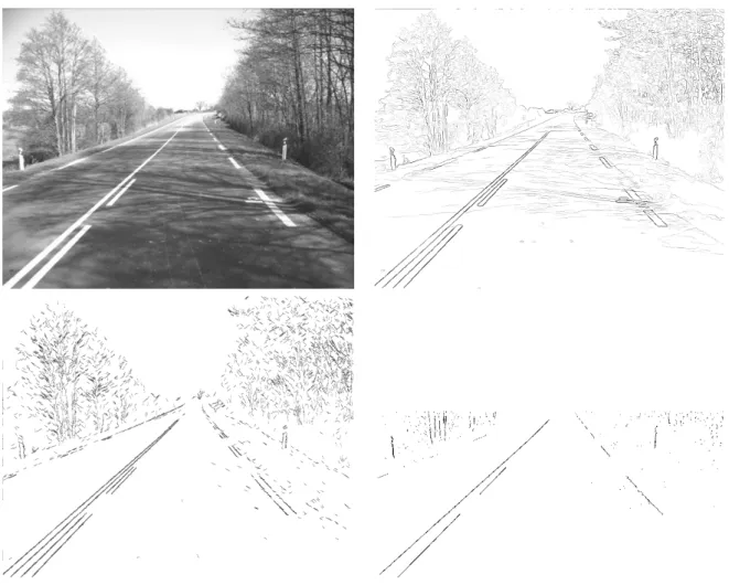
Figure 1.2: Top left: Original image of a road.
Top right: result of Canny’s filter.
Bottom left: result of Segment extraction [16].
Bottom right: result with the proposed lane-marking feature extractor (in this case, only the medial axis of each detected region is shown)
Finally, the centers of the selected couples of edges are used as features. The algorithm for every image line is:
• y = 1
• While y < ImageLineSize,
1. Compute the horizontal gradient G(y) 2. If G(y) > SG then,
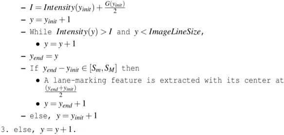
Robust Lane Marking Detection by the Half Quadratic Approach
– I= Intensity(yinit) +G(y2init)
– y= yinit+ 1
– While Intensity(y) > I and y < ImageLineSize, • y = y + 1
– yend= y
– If yend− yinit∈ [Sm, SM] then
• A lane-marking feature is extracted with its center at
(yend+yinit)
2
• y = yend+ 1
– else, y= yinit+ 1
3. else, y= y + 1.
Figure 1.2 shows the superiority of the proposed extractor w.r.t classical edge detectors in an adverse situation. The proposed extractor only yields a small number of outliers despite shadows and highlighted areas. Moreover the lane-markings are completely extracted. Note that extracting the center of the road marking rather than its edges avoids selecting redundant information that would be useless for the next processing steps.
1.4.2
Band Extraction
-0.5 1
2S 2S 2S
Figure 1.3: Band filter for marking extraction
When a road marking is dirty or worn-out, the condition Intensity(y) > I may not always be verified along its whole surface, and the previous extractor may not be able to completely extract it. This is why, following Thomas Veit’s (LIVIC) suggestions, we propose a new extractor based on the line convolution with the band filter shown in Fig. 1.3. As previously, the extractor processes every line of the image in a sequential fashion. Note that the convolution with the filter can be performed in only 4 operations: 4S1(3(C(y + S) −C(y − S)) − (C(y + 3S) −C(y − 3S))), independently of its width 6S, by using the cumulative function C(y) of the intensity profile along the line. The convolution is performed with several widths and the obtained results are summed. Finally, the local maxima of the summed convolutions are considered as putative marking centers and used as features. The algorithm for every image line is:
• C(0) = 0
– C(y) = C(y − 1) + Intensity(y − 1), – convsum(y) = 0
• For S = Sm/2 to SM/2,
– For y= 3S to ImageLineSize − 3S,
∗ convsum(y)+ =4S1(3(C(y + S) −C(y − S)) − (C(y + 3S) −C(y − 3S)))
• For y = 3S to ImageLineSize − 3S,
– if (convsum(y) ≥ convsum(y + 1)) and (convsum(y) ≥ convsum(y − 1)) a
lane-marking feature is extracted with its center at y.
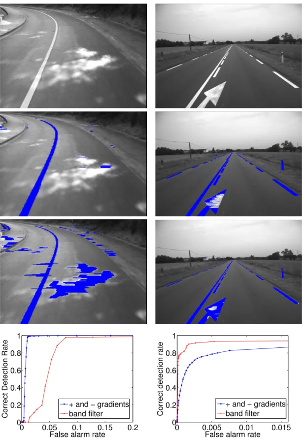
In figure 1.4, a comparison of the positive-negative gradients and band filter extractors is shown. The same parameters are used by the two extractors. On the first row, two original images are displayed and in the two following rows, areas extracted as marking appears in blue. A search for the best S given a center position was thus added after filter band extraction. In the last row, Receiver Operating Characteristic (ROC) curves are given. ROC curves display the false alarm rate versus the correct detection rate and allows to compare extractor performances independently of the value of the threshold parameter. While the positive-negative gradients extractor does not extract highlighted areas, it is not always able to extract dirty or erased mark-ings. On the contrary, the band filter extractor performs better on dirty or erased markings, but highlighted areas are also extracted as markings. As a consequence, to follow the conservative assumption, i.e., to avoid missing any feature, the band filter must be preferred.
1.5
Road Shape Model
In this section, we describe the curve model we use for aggregating the detected features into marking lines. This model is more detailed in [36].
In many road inventory and driving assistance systems, the marking detection has to be performed over a distance of 10 to 40m. Therefore, a flat road model, which neglects the vertical curvature of the road, seems to be a reasonable approximation. Its main advantage is that it allows the road shape to be estimated from only one camera. The road shape features are given by the lane-marking centers extracted as explained in Section 1.4. We assume that the extracted features are noisy measurements of a curve explicitly described by a linear parametric model: ˜ y= d
∑
i=0 fi(x) ˜ai= X(x)tA˜, (1.2)where(x, ˜y) are the image coordinates of a point on the curve, ˜A= ( ˜ai)0≤i≤d is the coefficient
vector of the curve parameters and X(x) = ( fi(x))0≤i≤d is the vector of basis functions of the
image coordinate x.
The linearity of this generative model (1.2) is particularly useful in setting up the shape estimation problem as a fitting problem and thus, in speeding up the detection. In practice, we model lane-markings on the road by polynomials y= ∑di=0aixi. While the clothoid model would
Robust Lane Marking Detection by the Half Quadratic Approach 0 0.05 0.1 0.15 0.2 0 0.2 0.4 0.6 0.8 1
False alarm rate
Correct Detection Rate
+ and − gradients band filter 0 0.005 0.01 0.015 0 0.2 0.4 0.6 0.8 1
False alarm rate
Correct detection rate
+ and − gradients band filter
Figure 1.4: First row: original images.
Second row: results of positive-negative gradients extractor. Third row: band filter extractor.
Fortunately, it can be well approximated with a polynomial as proposed in [12]. Moreover, the image of a polynomial on the (flat) road under perspective projection is a hyperbolic polynomial with equation y= c0x+ c1+ ∑di=2(x−xcih)i, where ciis linearly related to aias detailed in [39, 36].
Therefore, a hyperbolic polynomial model can also be used for a frontal camera. In this case, however, hyperbolic polynomials may advantageously be replaced by the so-called fractional
polynomials, defined by y= ∑d i=0dix
i
d, for the sake of numerical stability.
To avoid numerical problems, a whitening of the data is performed by scaling the image in a[−1,1] × [−1,1] box for polynomial curves and in a [0,1] × [−1,1] box for fractional polyno-mials, prior to the fitting.
In model (1.2), the vertical coordinate x is assumed non-random. Thus only the second coordinate of the extracted point, y, is considered as a noisy measurement:
y= X(x)tA˜+ b (1.3) In all that follows, the measurement noise b is assumed independent and identically distributed (iid), and centered. In the next section, we explain how the road shape model can be robustly fitted for lane-marking detection in images.
1.6
Parameters Estimation
In this section, we first review Least Squares fitting, then our approach to robust fitting is de-tailed within a Lagrangian formalism.
1.6.1
Least Squares Fitting
First, we recall the very simple situation where the noise b is Gaussian. The goal is to estimate the curve parameters ALS on the whole set of n extracted points (xi, yi), i = 1, ..., n. Let ˜A
denote the vector of “true” underlying curve parameters. Letσ be the standard deviation of the Gaussian noise b. The probability of a measurement point (xi, yi), given the curve parameters
A, or likelihood, is: pi((xi, yi)/A) = 1 √ 2πσe −12( XtiA−yi σ )2.
For the sake of simplicity, from now on, we note Xi= X(xi). We can write the probability of
the whole set of points as the product of the individual probabilities:
p∝ 1 σn i=n
∏
i=1 e−12( XtiA−yi σ )2, (1.4)where ∝ denotes the equality up to a factor. Maximizing the likelihood, p, is equivalent to minimizing the negative of its logarithm w.r.t A. In the Gaussian case, this leads to minimizing the so-called Least Squares error:
eLS(A) = 1 2σ2 i=n
∑
i=1 (XitA− yi)2.Robust Lane Marking Detection by the Half Quadratic Approach
The minimization of eLS is equivalent to solving the well-known normal equations:
X XtA= XY, (1.5)
where Y = (yi)1≤i≤n is the vector of y coordinates, the matrix X = (Xi)1≤i≤n is the design
matrix, and S= XXt is always symmetric and positive. If S is not singular, (1.5) admits the unique solution ALS= S−1XY. Computing the best fit ALS simply requires solving the linear
system (1.5). As just explained, it is also the Maximum Likelihood Estimate (MLE) assuming Gaussian noise.
Since Y only is random, the expectation of ALSis E[ALS] = S−1X E[Y ]. The point coordinates
in E[Y ] correspond to points exactly on the underlying curve ˜Y, thus ˜A= S−1X ˜Y. Therefore,
E[ALS] equals ˜A, i.e. the estimator ALS of ˜Ais unbiased.
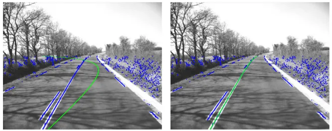
Figure 1.5: Road marking features (in blue) and estimated lane-marking (in green) assuming
Gaussian noise (left image) and T-Student noise, as defined in Sec. 2.2 (right image)
As is well known (see Figure 1.5), Least Squares fitting does not provide correct fits in the presence of image perturbations.
1.6.2
Robust Parameters Estimation
We still assume that the noise is iid and centered. But now, the noise is assumed to be non Gaussian. In particular, it may exhibit heavier tails than the Gaussian probability distribution function (pdf). It can be chosen in one of the families that will be presented in Chapter 2. The assumed noise model is specified by a function φ(t) in such a way that the probability of measurement point(xi, yi), given curve parameter A, is:
pi((xi, yi)/A) ∝ 1 se −1 2φ(( XtiA−yi s ) 2) (1.6)
In this Section, we revisit the derivation of the estimate using a Lagrangian approach which leads to the same algorithm as that obtained by the half-quadratic or M-estimation approach. The advantage of the Lagrangian framework is to allow a simple proof of local convergence and an interpretation in terms of dual optimization. As in the half-quadratic approach [14, 6], φ(t) satisfies the following hypotheses:
• H0: defined and continuous on [0,+∞[ as its first and second derivatives, • H1: φ′(t) > 0 (thus φ is increasing),
• H2: φ′′(t) < 0 (thus φ is concave).
These three assumptions are very different from those used in the M-estimation approach for the convergence proof. Indeed in [20], the convergence proof requires that potential function ρ(u) = φ(u2) be convex. In our case, the concavity and monotony of φ(t) implies that φ′(t) is bounded, but potentialφ(u2) is not necessarily convex w.r.t. u. Note that the smooth exponential
family (for α < 1) and the generalized T-Student family (for 0 < β) that will be presented in Chapter 2, both satisfy these three assumptions.
As stated in [20], the role of this functionφ is to saturate the error in case of a large scaled residual|bi| = |XitA− yi|, and thus to lower the importance of outliers. The scale parameter, s,
sets the residual value from which a noisy data point has a good chance of being considered as an outlier.
In the MLE framework, the problem is set as the minimization w.r.t. A of the robust error:
eR(A) = 1 2 i=n
∑
i=1 φ((X t iA− yi s ) 2). (1.7)Notice that while the Gaussian case would correspond to the particular case in whichφ(t) =
t, this function does satisfy assumption H2. eLS(A) is indeed a limit case of eR(A). Unlike in the
Gaussian case, the minimization problem is not quadratic. It could be solved iteratively using Gradient or Steepest Descent algorithms. However, these algorithms can be relatively slow around local minima, when the gradient slope is near zero. Indeed, their speed of convergence is only linear, while Newton algorithms achieve a quadratic speed of convergence. But generally, with Newton algorithms, the convergence to a local minimum is not certain. However, we prove that the Newtonian construction presented in the next paragraph always converges toward a local minimum. A global minimum could be obtained using simulated annealing, but at a much greater computational cost.
In the two following sections, we present the algorithm derived from (1.7) within Lagrange’s formalism. The approach consists in first rewriting the problem as the search for a saddle point of the associated Lagrange function. Then, the algorithm is obtained by alternated minimiza-tions of the dual function. As we will see, this algorithm corresponds to the well known algo-rithm named Iterative Reweighted Least Squares (IRLS).
1.6.3
Iterative Reweighted Least Square (IRLS)
First, we rewrite the minimization of eR(A) as the maximization of −eR. This will allow us
later to write −eR(A) as the extremum of a convex function rather than a concave one, since
the negative of a concave function is convex. Second, we introduce the auxiliary variables
wi = (X
t iA−yi
s )
2. These variables are needed to rewrite −e
R(A) as the value achieved at the
minimum of a constrained problem. This apparent complication is in fact valuable since it allows us to introduce the Lagrange multipliers. Indeed using H1, −eR(A) can be seen as the
Robust Lane Marking Detection by the Half Quadratic Approach
minimization w.r.t. W = (wi)1≤i≤n of:
E(A,W ) =1 2 i=n
∑
i=1 −φ(wi),subject to n constraints hi(A,W ) = wi− ( XitA−yi
s )
2
≤ 0. The following algorithm is derived from this constrained optimization problem as shown in appendix 6.1. The IRLS algorithm is:
1. Initialize A0, and set j= 1,
2. For all indexes i (1≤ i ≤ n), compute the auxiliary variables wi, j = (X
t iAj−1−yi
s )
2 and the
weightsλi, j = φ′(wi, j),
3. Solve the linear system ∑ii=n=1λi, jXiXitAj= ∑ii=n=1λi, jXiyi,
4. IfkAj− Aj−1k > ε, increment j, and go to 2, else ARLS= Aj.
The convergence test can also be performed on the error variation. A test on a maximum number of iterations can also be added.
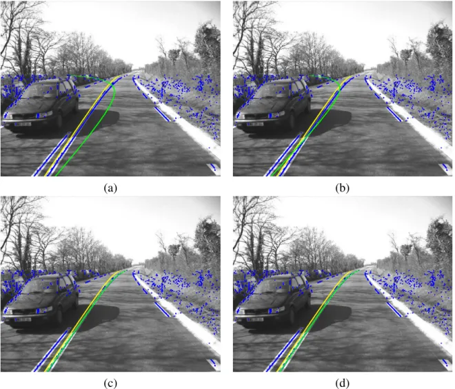
Finally, Figure 1.6 illustrates the importance of robust fitting in images with many outliers. The yellow lines depict the initial A0’s. The green ones are the fitting results AR, assuming
Gauss, smooth Laplace, Cauchy, and Geman & McClure [15] noises (as defined in the next chapter). A correct fit is achieved only with the last two pdfs, which correspond to non-convex potentials. This illustrates the importance of the choice of a noise model, as detailed in the next chapter.
1.7
Conclusion
We described the design of a camera-based lane-marking detection system involving a feature extraction step followed by a robust fitting step. The feature extraction takes into account the lane-marking geometry, particularly its width. This criterion allows us to better select features while following the conservative assumption, which means that outliers are removed even if very noisy data must be kept. These features are robustly fitted by a curve, using the well-known Iterative Reweighted Least Squares algorithm. We have shown how Lagrange multipliers lead to a revised half-quadratic theory and justify the local convergence of the algorithm even for non-convex potential, unlike M-estimators. Indeed, the half-quadratic framework is valid for a large class of non-convex potentials which leads to more robust estimators.
(a) (b)
(c) (d)
Figure 1.6: Fitting on a real image assuming Gauss (a), smooth Laplace (b), Cauchy (c), and
Geman & McClure (d) noise pdfs. Data points are shown in blue, yellow lines are the initial A0’s and green lines are the fitting results. The noise models used in this experiment are defined
Chapter 2
Modeling Non-Gaussian Noise
2.1
Introduction
In computer vision, data are most of the time corrupted by non-Gaussian noise or outliers and may contain multiple statistical populations. It is a difficult task to model observed per-turbations. Several parametric models were proposed in [19, 35], and sometimes based on mixtures [18]. Non-Gaussian noise models imply using robust algorithms to reject outliers. The most popular techniques are Least Median Squares (LMedS), RANSAC and Iterative Reweighted Least Squares (IRLS). The first two algorithms are close in their principle and achieve the highest breakdown point, i.e. the admissible fraction of outliers in the data set, of approximately 50%. However, their computational demand quickly increases with the number of parameters. We focus on the IRLS algorithm and one may argue that it is a deterministic algorithm that only converges towards a local minimum close to its starting point, as explain in the previous chapter. This difficulty can be circumvented by the so-called Graduated Non Convexity (GNC) strategy, that will be presented in this chapter. The IRLS algorithm, even within the GNC strategy, usually remains faster compared to LMedS and RANSAC and is also able to achieve the highest breakdown point.
We now rewrite (1.3), and thus let us consider the linear problem:
Y = XA + B (2.1)
where Y = (y1, ···,yn) ∈ Rn is a vector of observations, X = (x1, ···,xn) ∈ Rn×d+1 the design
matrix, A∈ Rd+1 the vector of unknown parameters that will be estimated by the IRLS algo-rithm, and B= (b1, ···,bn) ∈ Rnthe noise. The noise is assumed independent and identically
distributed but not necessarily Gaussian. We consider the fixed design setting, i.e. in (2.1),
X is assumed non-random. In that case, as demonstrated in [30], certain M-estimators achieve the maximum possible breakdown point. However, if X cannot be assumed non-random, the breakdown point of M-estimators drops towards zero [28]. This underlines the importance of the way computer vision problems are formulated.
This chapter is organized as follows. In Section 2.2, we present the non-Gaussian noise models we found of interest for lane-marking detection. Then in Section 2.3, we prove that M-estimators that achieve the maximum breakdown point of approximately 50% can be built based on these probability distribution families. This choice may have important consequences in terms of the sensitivity of the fitting result to the tuning of the parameters, especially when it
leads to a non-convex minimization. In Section 2.4 and Section 2.5, we also address this ques-tion and propose methods for automatically estimating these parameters. Finally, we describe advantages of so-called Graduated Non Convexity (GNC) strategy in Section 2.6. Most of this chapter was first published in [22, 26, 24].
2.2
Non-Gaussian Noise Models
We are interested in parametric functions families that allow a continuous transition between different kinds of probability distributions.
We here focus on two simple parametric probability density functions (pdf) of the form
pd f(b) ∝ e−ρ(b) suitable for the IRLS algorithm, where∝ denotes the equality up to a factor. Compared to the previous chapter, where the pdf was written as a function of φ, see (1.6), we use in this chapter mainly the ρ notation, for a better compatibility with Mizera and M¨uller’s work [30].
A first interesting family of pdfs is the stretched exponential family (also called generalized Laplacian, or generalized Gaussian [35]):
Eα,s(b) =
α
sΓ(2α1 )e
−((b
s)2)α (2.2)
The two parameters of this family are the scale s and the power α. The latter specifies the shape of the noise model. Moreover,α allows a continuous transition between two well-known statistical laws: Gaussian (α = 1) and Laplacian (α = 12). The associatedρ function is ρEα(
b s) =
((bs)2)α. The associatedφ function is φEα(t) = t
α, with t =b2 s2.
As detailed in Chapter 1, to guarantee the convergence of IRLS, theφ′function, related to ρ′ byφ′(u2) = ρ′(u)
2u with u= b
s, has to be defined on[0, +∞[. This is not the case for α ≤ 0 in
the stretched exponential family. Therefore, the so-called smooth exponential family (SEF) Sα,s
was introduced in [40]: Sα,s(b) ∝ 1 se −1 2ρα( b s) (2.3)
whereρα(u) =α1((1 + u2)α− 1). The associated φ function is φSα(t) =
1
α((1 + t)α− 1).
Table 2.1: list of noise models used in robust fitting (SEF)
α φSα(t) weight=φ′Sα(t) pdf name 1 t 1 Gauss 1 2 2( √ 1+ t − 1) √1 1+t smooth Laplace
0 (not defined) 1+t1 generalized T-Student
−1 (1+t)t
1
(1+t)2 Geman & McClure
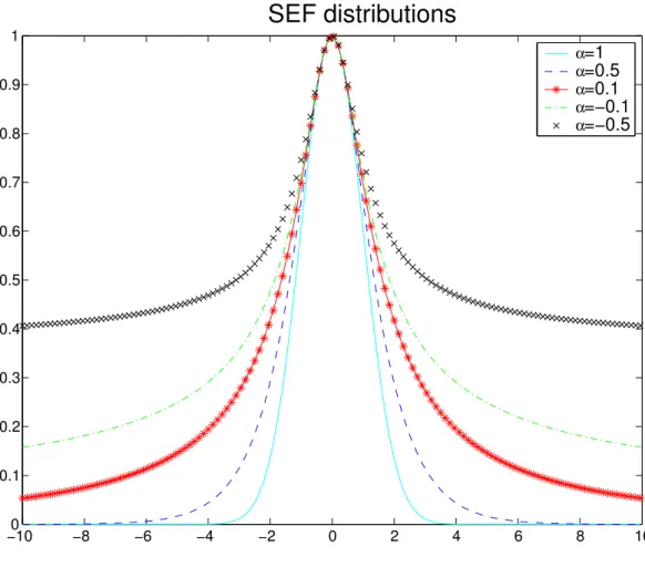
As for the stretched exponential family, α allows a continuous transition between well-known statistical laws such as Gauss (α = 1), smooth Laplace (α = 12) and Geman & McClure (α = −1), see Tab. 2.1. These laws are shown on Figure 2.1. Note that, for α ≤ 0, Sα,s can
Robust Lane Marking Detection by the Half Quadratic Approach −100 −8 −6 −4 −2 0 2 4 6 8 10 0.1 0.2 0.3 0.4 0.5 0.6 0.7 0.8 0.9 1
SEF distributions
α=1 α=0.5 α=0.1 α=−0.1 α=−0.5Figure 2.1: SEF noise models, Sα,s. Notice how tails are getting heavier asα decreases
be always normalized on a bounded support, so it can still be seen as a pdf. In the smooth exponential family, whenα is decreasing, the probability to observe large, not to say very large errors (outliers), increases.
In the IRLS algorithm, the residual b is weighted byλ = φ′(bs22). For the SEF, the associated weight isφ′S
α = (1 + t)
α−1, see Tab. 2.1. Notice that while the pdf is not defined whenα = 0,
its weight does and it corresponds in fact to the T-Student law. We define the Generalized T-Student Family (GTF) by:
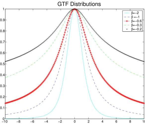
Tβ,s(b) = √ Γ(−β) πΓ(−β −12)s (1 +b 2 s2) β (2.4)
where β < 0. This family of pdfs also satisfies the required properties for robust fitting. It is named generalized T-Student pdf [19] in the sense that an additional scale parameter is intro-duced compared to the standard T-Student pdf. Notice, that the caseβ = −1 corresponds to the Cauchy pdf. These laws are shown in Figure 2.2. The GTF can be rewritten as:
Tβ,s(b) ∝1
se
−1
−100 −8 −6 −4 −2 0 2 4 6 8 10 0.1 0.2 0.3 0.4 0.5 0.6 0.7 0.8 0.9 1 β β β β β
GTF Distributions
=−2 =−1 =−0.6 =−0.3 =−0.2Figure 2.2: GTF noise models, Tβ,s. Notice how tails are getting heavier when β is increasing
towards0
where ρβ(bs) = −2βln(1 +bs22). The associated φ function is φTβ(t) = 2βln(1 + t). Moreover, it is easy to show that the so-called generalized T-Student pdfs have the same weight function
1
1+b2
s2
up to a factor.
The parameters of the GTF are s andβ (β < 0). They play exactly the same role as s and α in the SEF. For−12 ≤ β < 0, as previously the pdf is defined only for a bounded support.
The most surprising thing about this family is that, even if the tails of the pdf, which are controlled by β, can be very different, the weights are the same up to a factor β: 1
1+t. The
robust fitting is thus achieved by running exactly the same algorithm, whatever the value ofβ. However,β plays an important role in covariance matrix estimation as explained in Chapter 3.
Robust Lane Marking Detection by the Half Quadratic Approach
2.3
Robustness Study
Following [30], in the fixed design case, the robustness of an M-estimator is characterized by its breakdown point, which is defined as the maximum percentage of outliers the estimator is able to cope with:
ε∗( ˆA,Y, X) =1
nmin{m : supY˜∈B(Y,m)k ˆA( ˜Y ,X)k = ∞}
(2.6)
where ˜Y is a corrupted data set obtained by arbitrary changing at most m samples (among the
n samples of the data vector), B is the set of all ˜Y: B(Y, m) = { ˜Y : card{k : ˜yk 6= yk} ≤ m}
and ˆA( ˜Y, X) is an estimate of A from ˜Y. It is important to notice that the previous definition is different from the one proposed in [17] which is not suited to the fixed design setting.
Mizera and M¨uller [30] also emphasize the notion of regularly varying functions, and de-scribed the link between this kind of regularity and robustness property. By definition, f varies regularly if there exists a r such that:
lim
t→∞
f(tb)
f(t) = b
r (2.7)
When the exponent r equals zero, the function is said to vary slowly, i.e. the function is heavily tailed.
We now assume that theρ function of the M-estimator follows the four following conditions: 1. ρ is even, non decreasing on R+ and non negative,
2. ρ is unbounded,
3. ρ varies regularly with an exponent r ≥ 0,
4. ρ is sub-additive: ∃L > 0, ∀t,s ≥ 0, ρ(s +t) ≤ ρ(s) + ρ(t) + L.
The main result proved in [30] is that the percentageε∗is bounded by a function of r:
Theorem. Under the four previous conditions onρ, and if r ∈ [0,1], then ∀ Y and X,
M(X, r)
n ≤ ε
∗( ˆA,Y, X) ≤M(X, r) + 1
n (2.8)
where, with the convention00= 0, M(X, r) is defined as:
M(X, r) = min A6=0{card(K) :k
∑
∈K|X t kA| r ≥∑
k∈K/ |XktA| r } (2.9)where K runs over the subsets of{1,2,···,n}.
When the exponent r is zero, the exact value of the percentageε∗is known. The following theorem states its value.
Theorem. Under the four previous conditions onρ and if r = 0, then ∀ Y and X, ε∗( ˆA,Y, X) = M(X, 0) n = 1 n⌊ n−
N
(X) + 1 2 ⌋ (2.10)where ⌊x⌋ represents the integer part of x, and
N
(X) = maxA6=0{card{Xk : XktA= 0},k =1, ···,n}.
This value is also the maximum achievable value, which is approximately 50%. As a con-sequence, M-estimators with zero r exponent achieve the highest breakdown point.
Finally in [30], it is shown that the bounds on the percentageε∗are related to r as a decreas-ing function. This is stated by the followdecreas-ing lemma:
Lemma. If q≥ r ≥ 0 then
M(X, q) ≤ M(X,r) ≤ M(X,0) = ⌊n−
N
(X
) + 12 ⌋.
These three results clearly establish the relationship between the exponent r of the function ρ and the robustness of the associated M-estimator. As a consequence of these important theo-retical results, the robustness of a large class of M-estimators can be compared just by looking at the exponent r of the cologarithm of their associated noise pdf. To illustrate this, we now apply the above results to the SEF and GTF pdfs described in Section 2.2.
2.3.1
The SEF case
Let us show that the robustness of SEF based M-estimators is decreasing withα ∈]0,0.5]. To this end, we first check the four above conditions on the ρα function. Function ρα is clearly
even, non decreasing on R+ and non negative. The first condition is thus satisfied. The second one is fulfilled only whenα > 0, due to the fact that ρα is bounded forα ≤ 0. Looking at the
ratio: ρα(tb) ρα(t) = (1 + t2b2)α− 1 (1 + t2)α− 1 = (1 t2+ b2)α−t12α (t12+ 1)α− 1 t2α
we see that whenα > 0, limt→∞ρραα(tb)(t) = b
2α. As a consequence, theρ
αfunction varies regularly
and the third condition is also satisfied. For the fourth condition, we can use Huber’s Lemma 4.2 [21], to prove the sub-additivity when α ∈]0,0.5[. For α = 0.5, it can also be proved that ρα is sub-additive. All conditions onρ being fulfilled, the first Theorem applies, and using the Lemma, we prove that the robustness of SEF M-estimators is increasing towards the maximum of approximately 50%, with respect to a decreasingα parameter within ]0, 0.5].
2.3.2
The GTF case
Let us prove that the robustness of GTF M-estimators is maximum, whatever the value of β. We shall first check the 4 conditions on the associatedρ function. The first two assumptions are easy to check forρβ. Looking at the ratio:
ρβ(tb) ρβ(t) = ln(t2) + ln(1 t2 + b2)) ln(t2) + ln(1 t2+ 1))
Robust Lane Marking Detection by the Half Quadratic Approach
we deduce: limt→∞ ρβ(tb)
ρβ(t) = 1 = b
0. As a consequence, the ρ
β function varies slowly, and the
third condition is fulfilled. The fourth condition is proved by using Huber’s Lemma 4.2 [21]. All conditions on ρ being satisfied, the second Theorem applies, showing that GTF M-estimators achieve the highest breakdown point of approximately 50%.
2.4
Noise Model Parameters Estimation
In the previous section, two noise models were proposed, which can achieve the 50% breakdown point. To use them in practical applications, it remains to estimate the scale s and the powerα orβ of the models from residuals obtained in images.
When the pdf support is unbounded and other noise parameters are assumed to be known, by deriving the negative log-likelihood w.r.t. s, we get the following implicit equation in ˆs:
ˆ s2= 1 n i=n
∑
i=1 φ′((X t iA− yi)2 ˆ s2 )(X t iA− yi)2 (2.11)This equation means that the MLE estimate ˆsof s is a fixed point. Other scale estimators such as MAD [17], have been proposed. In the case of a bounded support, a more complex equation, involving the integral of the pdf on its support, can also be derived.
Interestingly, when the stretched exponential family (2.2) is used, (2.11) is simplified and gives the following closed-form estimator:
ˆ s= (2α n i=n
∑
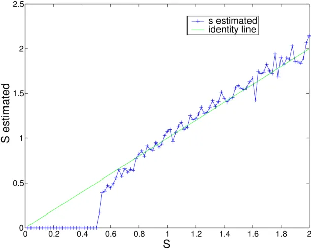
i=1 b2αi )2α1 (2.12) The MLE estimator of the scale must be used with care. Surprisingly, for low noise levels, we observed that the scale is clearly under-estimated. This is a general problem, due to the finite precision of feature detectors (in our case, it provides discrete image positions). In Figure 2.3, we simulate this effect by generating a Cauchy noise (β = 1) with increasing scales, and round-ing it. Then, the MLE scale ˆsestimate is computed from this data, assuming a Cauchy noise with unknown scale in (2.11). Figure 2.3 confirms our observation: when the true scale s is lower than one pixel, it is clearly under-estimated.This suggests that during its estimation, the scale must not been allowed to take small values ( i.e. lower than one pixel). This also implies that it is better not to estimate the scale between each step of the robust fitting, in contrast to what was suggested in [20]. Indeed, an under-estimated scale can freeze the fit in its current state, while it has not yet converged, as explained in Section 2.6.
The MLE approach, when applied to the estimation ofα or β, assuming a known s, does not seem to yield close-form estimators. Nevertheless, this estimation may always be performed by numerically minimizing the likelihood w.r.t.α, using for example a Gradient Descent algorithm. The MLE approach can also be applied to estimateα and s at the same time by a non-linear minimization as shown in Figure 2.4 where residuals are collected from a set of 150 images. In other experiments, we also typically obtained small scale estimates, due to the feature extractor, and values of α near zero. Since s is relatively small compared to the size of the image, the quantized data provided by the lane-marking extractor may thus produce an under-estimated s.
0 0.2 0.4 0.6 0.8 1 1.2 1.4 1.6 1.8 2 0 0.5 1 1.5 2 2.5
S
S estimated
s estimated identity lineFigure 2.3: The estimated scale ˆs versus the true scale s for Cauchy noise. We can notice that s is under-estimated by the MLE estimators when sˆ < 1, due to data rounding
As for the MLE estimator of s, the MLE estimator of(α, s) must be used with caution. Indeed, there are singular sets of residuals wereα and s can not be estimated properly.
Finally, to estimate( ˆs, ˆα), we can envision three different approaches to collect the residuals: 1. Collect residuals from a large set of images that are statistically representative of the application. Estimate the noise parameters and use them as fixed values in the curve fitting algorithm.
2. Collect residuals from each image after fitting (using averaged noise parameters). Refine the curve fit with the obtained noise model parameters.
3. When processing an image sequence, collect residuals from the m previous images and use them to estimate the noise parameters. Then perform curve fitting on the current image using the previously estimated parameters, assuming a temporal continuity. The first approach seems to be convenient for pure recognition or detection problems in a single image. But when tracking is involved, noise parameters are not constant in time. Thus,
Robust Lane Marking Detection by the Half Quadratic Approach −200 −150 −100 −50 0 50 100 150 200 −10 −9 −8 −7 −6 −5 −4 −3 −2
Log histogram fit
residual
log(probability)
Figure 2.4: Log histogram of the residual errors in feature position collected from 150 images
after lane-marking fits. With the MLE approach, this distribution is well approximated by the best fit in the SEF (2.3) with parametersα = 0.05 and s = 1.9
the second approach seems more attractive. Nevertheless, it may lead to bad estimates of the noise parameters in case of an image without lane-marking. Therefore from our experiments, we conclude that the third approach should be adopted.
2.5
Sensitivity of Fitting to Noise Model Parameters
By their very nature, robust fitting algorithms are not very sensitive to outliers. However, an-other question of importance is their robustness to an inappropriate choice of the noise model parameters. In order to evaluate the effect of this kind of modeling error on the fitting, we ran the following experiment:
1. We collect a set of 150 images showing the same lane-marking in the same position but with different perturbations (some of which are shown in Figure 2.5).
Figure 2.5: Six of the 150 images used in the experiments. The black straight line is the reference
Robust Lane Marking Detection by the Half Quadratic Approach
2. The reference lane-marking was accurately measured by hand. In this experiment fits are straight lines.
3. For each image of the set, fits were estimated for pairs of(α, s) on a grid assuming a noise model in the smooth exponential family.
4. The relative error between the fits and the reference fit was averaged over the image set for each(α, s). Figure 2.6 shows the obtained results.
On the top of Figure 2.6, with a random initialization, we observed that the valley along a α cross-section is very wide compared to an s cross-section. Moreover, when the initialization is set in the vicinity of the reference as on the bottom of Figure 2.6, the error function between the fit and the reference for differentα and s is very flat for α < 0. This is important to notice, since it means that whenα is chosen in the range of correct values, s can vary over a large range without really modifying the resulting fits. This can also be understood by the fact that the SEF (2.3) behaves approximately like the stretched exponential family (2.2). And as noticed in [3], the interesting fact with the stretched exponential family is that the obtained fits are invariant with respect to the value of s. Indeed, the weights computed in step 2 of the robust fitting algorithm areλi= 2α
b2i(α−1)
s2(α−1). Thus, step 3 is not modified whatever the value of s, since
s2(α−1)can be simplified on the left and right hand sides after substitution of the weights. Least
Squares Fitting shares the same invariance property as explained in Section 1.6.1. A similar argument can be used to show that the robust fitting algorithm is invariant toβ when the noise model is chosen in the generalized T-Student family.
To summarize, the robust fitting algorithm with a noise model chosen from the SEF is, in our context, relatively robust to the scale parameter s but less robust to errors on the power parameterα. With the GTF noise model, the robust fitting algorithm is invariant to the choice ofβ.
2.6
Improving Convergence: the GNC Strategy
The relative robustness of the curve fitting observed in the previous section can be exploited to speed up the convergence toward a local minimum and to help select a local minimum close to the global one.
Figure 2.7 shows that the weight λ, used in the IRLS algorithm, becomes more sharply peaked when α or s decrease. As a consequence, the lower α or s, the lower the effect of outliers on the result and thus, the more robust the fitting.
Thus, whenα decreases, the robust error function eR(A) becomes less and less smooth. If
α = 1, the cost function is a paraboloid and thus there exists a unique global minimum. By decreasingα to values lower than 12, local minima appear (when curve is with more than one parameter, d+ 1 > 1). This is illustrated in Figure 2.8 where the robust error function eR(A) is
shown for three decreasing values ofα.
As explained in [2], the localization property of the robust fitting w.r.t. decreasing α can be used to converge toward a local minimum close to the global one. This approach, called Graduated Non Convexity (GNC), consists in, first, enforcing local convexity on the data using a large value of α. Then, a sequence of fits with decreasing α, is performed in continuation,
−1 −0.5 0 0.5 1 0 2 4 6 8 10 12 14 16 18 20 0 0.1 0.2 0.3 0.4 0.5 α Parameters Fitting relative error
s 0.05 0.1 0.15 0.2 0.25 0.3 0.35 0.4 0.45 −1 −0.5 0 0.5 1 0 5 10 15 20 0 0.1 0.2 0.3 0.4 0.5 α Parameters fitting relative error
s 0.01 0.02 0.03 0.04 0.05 0.06 0.07 0.08 0.09 0.1
Figure 2.6: Errors between the fit and reference for different α and s. Top, the initial curve
parameters A0 are set to random values; bottom, A0 is set in the vicinity of the reference.
Robust Lane Marking Detection by the Half Quadratic Approach −100 −8 −6 −4 −2 0 2 4 6 8 10 0.1 0.2 0.3 0.4 0.5 0.6 0.7 0.8 0.9 1 b λ α =1 α =0.5 α =−0.5 α =−1.5 −100 −8 −6 −4 −2 0 2 4 6 8 10 0.1 0.2 0.3 0.4 0.5 0.6 0.7 0.8 0.9 1 s=0.2 s=1 s=2 s=3 λ b
Figure 2.7: Variations of weight λ with respect to the residual error b, top for s = 2.4 and
0 50 100 150 200 250 −0.2 −0.15 −0.1 −0.05 0 0.05 0.1 0.15 0.2 0 2 4 6 8 x 10⁶ slope position 1 2 3 4 5 6 7 x 10⁶ 0 50 100 150 200 250 −0.2 −0.1 0 0.1 0.2 500 1000 1500 2000 2500 slope position 600 800 1000 1200 1400 1600 1800 2000 0 50 100 150 200 250 −0.2 −0.15 −0.1 −0.05 0 0.05 0.1 0.15 0.2 70 80 90 100 110 slope position 80 85 90 95 100 105
Figure 2.8: The robust error function eR(A) for the two parameters of a straight line for different
values ofα: Gaussian noise (α = 1), near T-Student noise (α = 0.1), Geman&McClure noise
Robust Lane Marking Detection by the Half Quadratic Approach
i.e. each time using the current output fit as an initial value for the next fitting step. But one must be careful not to decreaseα or s too fast. Indeed, with too small an α or s, the number of local minima increases and the curve fitting algorithm has a higher chance of being trapped into a local minimum located far from the global one. In practice, this implies that the estimated curve parameters are frozen at their current values during the alternate minimization [9]. As a conclusion, the lower bound of the decreasing α must not be too small compared to the ˆα estimated from the residuals as explained in Section 2.4.
An increasing scale s has the same smoothing effect on the robust error as an increasing α. Thus, as proposed by [32], large scales can be used similarly to high α to converge to a local minimum that is close to the global one and to speed up the convergence. On the other hand, when too small a value of s is chosen, the curve parameters can also be frozen to their current values during the fit. Therefore, to maintain good convergence properties and to have an algorithm that is as fast as possible, the MLE estimate ( ˆs, ˆα) helps us to select the correct values for the lower bounds of a sequence of decreasing s andα.
2.7
Conclusion
In this chapter, the important question which we have addressed is the choice of the noise
distribution model parameters. We have introduced two-parameter families of noise models that allow a continuous transition between the Gaussian model and non Gaussian models. We have showed how this last property can be used to improve fitting results and robustness: even with a slightly incorrect noise model of these families, the estimated fits remain relatively reliable.
Moreover, we applied Mizera and M¨uller’s fundamental work on M-estimators breakdown point calculation in the field of image analysis. In the fixed design setting, they shown that certain M-estimators can achieve maximum robustness. Using their results, we discussed the robustness of M-estimators based on two non-Gaussian pdfs families, that we introduced under the names of SEF and GTF. In particular, we showed that the GTF noise model leads to M-estimators that achieve the maximum breakdown point of approximately 50%, and that the robustness associated with SEF increases towards the maximum asα decreases towards 0.
To finish, we illustrated how useful these results are for lane-marking detection: SEF and GTF approximate models seems to correctly fit observed noise pdfs. The sensitivity to noise parameters appears to be good, especially when using the GNC approach. We therefore believe that the SEF and GTF families can also be used with advantages in many other image analysis algorithms.
Chapter 3
Evaluating the Fits and Tracking
3.1
Introduction
In practical applications, an estimate must be accompanied by some measure of confidence in order to be correctly used by higher level systems, such as Kalman filters in tracking appli-cations. In the statistical estimation framework, this confidence measure is naturally given by (the inverse of) the covariance matrix. That is the main reason why we formulated detection as a fitting problem in Chapter 1. With Gaussian noise, computing the covariance matrix is straightforward, see Section 3.2.
In the robust framework, however, a correct covariance matrix estimate is more difficult to obtain. There are two main reasons for this. First, there is no known closed-form solution, but only approximations. In this chapter, we focus on approximations that can be quickly computed from the data in hand during the fitting. Second, it turns out that an accurate choice of the noise model is much more critical for the covariance matrix estimation than for the fitting. Despite these difficulties, we are able to propose fast-to-compute and efficient approximates of the covariance matrix as explained in Section 3.3.
In the last two sections, for an intuitive understanding, we make a gradual presentation of the robust Kalman framework which is useful for implementing tracking along an image sequence. In Section 3.4, we introduce recursive and robust least squares (recursive least squares is a simple case of Kalman filter, using a constant state model). Finally in Section 3.5, the robust Kalman filter is described. This Chapter was partially published in [40, 23].
3.2
Exact Covariance Matrix for Least Squares Fitting
Using notations of Section 1.6.1, the covariance matrix CLSof Least Squares Fit ALSis E[(ALS−
E[ALS])(ALS− E[ALS])t] = S−1X E[(Y − E[Y ])(Y − E[Y ])t]XtS−t. We have E[(Y − E[Y ])(Y −
E[Y ])t] = σ2I
n×n, since the noise b is iid with varianceσ2, where In×ndenotes the n× n identity
matrix. Finally, the inverse covariance matrix of ALSis deduced as:
CLS−1= 1
σ2S= QLS (3.1)
QLS is also known as Fisher’s information matrix for the set of n data points. QLSis defined as
Finally, it is important to notice an interesting property of Least Squares fitting: the fit does not rely on a correct estimate of σ. σ is requested only for computing the covariance matrix. Therefore,σ is generally estimated just before covariance matrix computation, from the residuals obtained after parameter fitting. The MLE estimator ofσ is obtained by canceling the first derivative w.r.tσ of −ln(p), which yields:
ˆ σ2=1 n i=n
∑
i=1 (XitALS− yi)2 (3.2)3.3
Approximate Confidence Matrices for Robust Fitting
A complete review of the many different approaches for approximating covariance matrices is beyond our scope here. Thus, we present a selection of five matrices that can be efficiently computed. Then, we propose a new approximation whose performances in terms of quality will be evaluated.
3.3.1
Available Approximates
The simplest approximate covariance matrix CCipra, named after Cipra’s covariance matrix
from [40], is: CCipra= s2 i=n
∑
i=1 λiXiXit !−1 ,where λi are the values taken by the weights after robust fitting converged. Another
fast-to-compute approximation is proposed in [40]:
CSimple= s2 i=n
∑
i=1 λ2iXiXit !−1 .Notice that in these two definitions, s2appears as a factor. As a consequence, incorrect values of the scale parameter lead to poor-quality estimates.
In chapter 7 of [20], Huber derives an asymptotic covariance matrix and proposes three other approximate covariance matrices:
CHuber1= K2 1 n−d−1∑ i=n i=1(ρ′(bi))2 (1 n∑ i=n i=1ρ′′(bi))2 i=n