Higher-Order Finite Elements for Hybrid Meshes Using New Nodal Pyramidal Elements

HAL Id: hal-00454261

https://hal.archives-ouvertes.fr/hal-00454261

Submitted on 8 Feb 2010

HAL is a multi-disciplinary open access

archive for the deposit and dissemination of

sci-entific research documents, whether they are

pub-lished or not. The documents may come from

teaching and research institutions in France or

abroad, or from public or private research centers.

L’archive ouverte pluridisciplinaire HAL, est

destinée au dépôt et à la diffusion de documents

scientifiques de niveau recherche, publiés ou non,

émanant des établissements d’enseignement et de

recherche français ou étrangers, des laboratoires

publics ou privés.

New Nodal Pyramidal Elements

Morgane Bergot, Gary Cohen, Marc Duruflé

To cite this version:

Morgane Bergot, Gary Cohen, Marc Duruflé. Higher-Order Finite Elements for Hybrid Meshes Using

New Nodal Pyramidal Elements. Journal of Scientific Computing, Springer Verlag, 2010, 42 (3),

pp.345–381. �10.1007/s10915-009-9334-9�. �hal-00454261�

HIGHER-ORDER FINITE ELEMENTS FOR HYBRID MESHES

USING NEW NODAL PYRAMIDAL ELEMENTS

Morgane Bergot

Projet POems, INRIA Rocquencourt, Le Chesnay, France Email: morgane.bergot@inria.fr

Gary Cohen

Projet POems, INRIA Rocquencourt, Le Chesnay, France Email: gary.cohen@inria.fr

Marc Durufl´e

Institut Math´ematique de Bordeaux, Universit´e Bordeaux I, Bordeaux, France Email: marc.durufle@math.u-bordeaux1.fr

Abstract

We provide a comprehensive study of arbitrarily high-order finite elements defined on pyramids. We propose a new family of high-order nodal pyramidal finite element which can be used in hybrid meshes which include hexahedra, tetrahedra, wedges and pyramids. Finite elements matrices can be evaluated through approximate integration, and we show that the order of convergence of the method is conserved. Numerical results demonstrate the efficiency of hybrid meshes compared to pure tetrahedral meshes or hexahedral meshes obtained by splitting tetrahedra into hexahedra.

Key words: pyramidal element, higher-order finite element, hybrid mesh, conformal mesh, continuous finite element, discontinuous Galerkin method, error estimates, quadrature for-mula.

Introduction

Highly efficient finite element methods using hexahedral meshes have been developed by Cohen [9] and his collaborators (Fauqueux [10], Pernet and Ferri`eres [11], [25], Durufl´e [13], [14]) but currently the only systematic way to generate unstructured hexahedral meshes for a complex geometry is to generate a tetrahedral mesh, and split each tetrahedron into four hexahedra, which introduce needlessly substantial increase in the cost. However, some mesh generators are able to produce hexahedral-dominant meshes that include a minor number of tetrahedra, wedges and pyramids. The aim here is to study finite element methods on hybrid meshes in order to preserve the efficiency of the method developed for hexahedra.

Nodal finite elements are detailed in Hesthaven and Teng [20] for tetrahedra, and Cohen [9] for hexahedra. Wedge (or triangular prism) nodal finite elements are constructed as a tensor product between Legendre-Gauss-Lobatto (LGL) points on [0,1] and electrostatic points on the triangle including LGL points on the edges [20]. In this work, the main effort is devoted to the construction of pyramidal finite elements, preserving conformity with the other types of elements.

Since obtaining a proper base for nodal pyramidal elements is a tricky point, two approaches have been attempted. A first approach consists in using rational functions in order to obtain nodal shape functions.

ˆ First works about nodal pyramidal elements have been made by Bedrosian in [2] where he

noticed the impossibility of choosing polynomial shape functions if we want to preserve the conformity with other elements. As a solution, he proposes what he calls “rabbit-functions” for first-order and second-order approximations. But, the second-order approx-imation does not include a node at the center of the quadrilateral base, which prohibits the conformity with the second-order hexahedron.

ˆ Zgainski et al. [33] perform numerical experiments with the basis functions given by

Bedrosian, and propose a modified second-order set of shape functions by adding a node at the center of the quadrilateral base. However, the central basis function proposed does not satisfy the nodal condition ϕi(Mj) = δij, and the modification does not improve the

accuracy, since the finite element space generated by this set of basis functions does not contain P2. The same idea is taken back by Graglia et al. [17] who achieve to improve

the accuracy with their own second-order central basis function.

ˆ Chatzi and Preparata [6] introduce a generalization of Bedrosian basis functions at any

order for nodes regularly distributed on the pyramid. Unfortunately, these basis functions are not consistent for order greater or equal to three since polynomials are not generated by these functions.

The second approach is to split the pyramid into tetrahedra to avoid the use of rational fractions, which have the debatable reputation to make the basis functions hard to manipulate, and instead use polynomial basis functions.

ˆ Wieners [31], Knabner and Summ [22], and Bluck and Walker [3] provide a consistent

first-order set of shape functions which ensures the conformity with tetrahedra and hexahedra, by splitting a pyramid into two tetrahedra. Second-order shape functions have been proposed by Wieners, and high order shape functions by Bluck and Walker. However, the finite element space of higher order does not contain the low order finite element space, which leads to a non-consistent method in the case of non-affine pyramids. Moreover, this method requires expensive quadrature on each tetrahedron.

ˆ Liu et al. [23] propose to symmetrize shape functions of Wieners, but this modification

barely improves the accuracy of the method.

An other popular alternative for finite element is the hp approach (Szab´o and Babuˇska [29]), e.g. with ˇSol´ın et al. [28] for hexahedra, tetrahedra and wedges. Several papers extend the hp finite element to pyramidal elements.

ˆ Warburton [30], Sherwin [26], Sherwin et al. [27], and Karniadakis and Sherwin [21]

provide a tensorial set of basis functions for all types of elements based on the degeneration of a cube. For tetrahedra, hexahedra and wedges, the generated finite element spaces are standards. For pyramids, the proposed generated finite element space provides an optimal convergence for affine pyramids, but not for distorted pyramids for an order greater or equal to two. Moreover, the continuous transition between pyramids and tetrahedra is not achievable for general unstructured meshes.

ˆ Nigam and Phillips [24] propose an original finite element space by deriving pyramidal

element space they obtain, the accuracy is preserved but the dimension of this space could be reduced.

ˆ Demkowicz et al. [12] and Zaglmayr [32] give the construction of partial-orthogonal basis

functions for tetrahedra, hexahedra and wedges, and exploit the use of a degenerated cube for pyramidal elements to get a finite element space that preserve the optimal accuracy, with a smaller dimension than Nigam and Phillips.

In this paper, the reference element is the symmetric unit pyramid (Fig. 1.1). Let Pr be

the polynomial space of degree r, we claim that if we choose the following finite element space ˆ

Pr = Pr(ˆx, ˆy, ˆz) ⊕ ∑ 0≤k≤r−1

(₁xˆˆ_{− ˆz)}y r−k Pk(ˆx, ˆy),

we are able to produce optimal error estimates in H1 norm ∣∣u − πru∣∣1,K≤ Chr∣∣u∣∣r+1,K

with the notations detailed in Section 4, for continuous finite elements.

In order to evaluate integrals, we propose in Section 3 to use the same technique as Bedrosian, detailed by Hammer, Marlowe and Stroud in [18], adapted to the pyramid and which does not deteriorate the accuracy, as it will be proved in Section 4. An extension of this work is proposed for discontinuous Galerkin formulation with the same finite element space ˆPr.

To validate this new pyramidal finite element, a dispersion analysis is carried out in the case of periodic meshes. We have observed an optimal dispersion error in O(h2r) as obtained for other element shapes. Furthermore these elements have been tested for the Helmholtz equation with the continuous Galerkin formulation, and for the unsteady wave equation with the discontinuous Galerkin method. The numerical experiments show that they are much more efficient than purely tetrahedral elements, or hexahedral meshes generated by splitting each tetrahedron into four hexahedra.

The outline of our paper is as follows:

ˆ In Section 1, following the classical notations of Ciarlet [7], we define two pyramidal finite

elements of order r, ( ˆK, ˆPr, ˆΣ) on the reference element, and (K,Pr,Σ) for any pyramid

in the mesh ;

ˆ A comparison to existing hp finite element spaces is given in Section 2, along with possible

improvements of these spaces, in propositions 2.2 and 2.3 ;

ˆ The quadrature formula used to get exact integrals, whenever it is possible, for the basis

functions constructed from the finite element space ˆPr are presented in Section 3, thanks

to a change of variable from the unit cube ;

ˆ Section 4 is devoted to the error analysis which is performed in a classical way ;

ˆ The case of a discontinuous Galerkin formulation is briefly treated in Section 5 ;

ˆ Section 6 is devoted to numerical results: a dispersion analysis is performed on the wave

equation in section 6.1, the stability condition (CFL) is computed on a periodic infinite mesh in section 6.2, and numerical experiments are performed in section 6.4 along with explanations about storage.

1. Arbitrary High-Order Pyramidal Element

1.1. Pyramidal Element

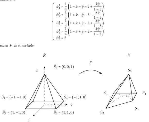
Definition 1.1 A pyramid K(x,y,z) is the image of the reference pyramid ˆK(ˆx, ˆy, ˆz) taken as the unit symmetrical pyramid, centered at the origin by the transformation F given by Bedrosian [2] using rational fractions, as shown in Fig. 1.1

F= ∑

1≤i≤5

Siϕˆ 1

i, (1)

where Si = (xi, yi, zi) are the vertices of the pyramid K and ˆϕ 1

i are the following mapping

functions ⎧⎪⎪⎪⎪ ⎪⎪⎪⎪⎪ ⎪⎪⎪⎪⎪ ⎪⎨ ⎪⎪⎪⎪⎪ ⎪⎪⎪⎪⎪ ⎪⎪⎪⎪⎪ ⎩ ˆ ϕ11= 1 4(1 − ˆx − ˆy − ˆz + ˆ xˆy 1− ˆz) ˆ ϕ12= 1 4(1 + ˆx − ˆy − ˆz − ˆ xˆy 1− ˆz) ˆ ϕ13= 1 4(1 + ˆx + ˆy − ˆz + ˆ xˆy 1− ˆz) ˆ ϕ14= 1 4(1 − ˆx + ˆy − ˆz − ˆ xˆy 1− ˆz) ˆ ϕ15= ˆz when F is invertible. ˆ K ˆ S1= (−1,−1,0) ˆ S2= (1,−1,0) ˆ S5= (0,0,1) ˆ S4= (−1,1,0) ˆ S3= (1,1,0) F ˆ z ˆ x ˆ y K S5 S1 S2 S3 S4

Fig. 1.1. Transformation of the reference pyramid ˆK_{to the pyramid K via the transformation F}

Remark 1.2 The mapping functions ˆϕ1_i are denoted with an upper index 1 as they correspond to the basis functions of order 1.

The case of a non-invertible transformation may occur when considering a degenerated element, e.g. when the five vertices are co-planar, but the characterization of pyramids for which F is invertible remains an open question, as for hexahedra (Durufl´e et al. [14]). In the sequel, we assume that F is always invertible.

The transformation F can be explicitly written as

4F= (S1+ S2+ S3+ S4) + ˆx (−S1+ S2+ S3− S4) + ˆy (−S1− S2+ S3+ S4)

+ ˆz (4S5− S1− S2− S3− S4) + xˆˆ

y

1− ˆz(S1+ S3− S2− S4). We notice that F is affine when

S1+ S3= S2+ S4,

i.e. when the base of the pyramid is a parallelogram. Furthermore, F ensures the conformity with tetrahedra and hexahedra as the shape functions becomes a two-dimensional triangular or quadrilateral shape function, since adjacent tetrahedra, wedge and hexahedra have the same property. That would not be the case if F had been chosen to be polynomial.

Remark 1.3 The shape function of Bedrosian can be found by defining the transformation T from the unit cube ̃Qto the reference pyramid ˆK

T ∶⎧⎪⎪⎪⎪⎨⎪⎪⎪ ⎪⎩ ˆ x= (1 − ̃z)(2̃x− 1) ˆ y= (1 − ̃z)(2̃y− 1) ˆ z= ̃z. (2)

For a basis function of the hexahedron ϕ(̃x, ̃y, ̃z) = (1 − ̃x)(1 − ̃y)(1 − ̃z), the transformation T gives indeed ϕ○ T−1(ˆx, ˆy, ˆz) = 1 4 (1 − ˆx − ˆz)(1 − ˆy − ˆz) 1− ˆz = ˆϕ 1 1(ˆx, ˆy, ˆz).

Similarly, we find the other functions of Bedrosian. 1.2. A Pyramidal Finite Element Space of Order r

We place ourselves in the most restrictive case, that is continuous finite elements. The finite element space Vh on an open set Ω of R

3

is given by Vh= {u ∈ H

1

(Ω) ∣ u∣K∈ PrF(K)},

where P_rF is the real space of order r for an element K of the mesh defined by P_rF(K) = {u ∣ u ○ F ∈ ˆPr( ˆK)},

The finite element space ˆProf order r on ˆK is

ˆ Pr(ˆx, ˆy, ˆz) = {ˆx i_ˆ yjzˆk, i+ j + k ≤ r} when ˆK is a tetrahedron ; ˆ Qr(ˆx, ˆy, ˆz) = {ˆx i_ˆ yjzˆk, i, j, k≤ r} when ˆK is a hexahedron ; ˆ Pr(ˆx, ˆy) ⊗ Pr(ˆz) = {ˆx i_ˆ yjzˆk, i+ j ≤ r,k ≤ r} when ˆK is a wedge ;

ˆ and defined by identity (5) when ˆK is a pyramid.

To use the Bramble-Hilbert’s lemma and get optimal error estimates, the real space PF r for

a pyramidal element K of the mesh must be such that

Theorem 1.4 When F is affine, the minimal space ˆProf order r such that we have the

inclu-sion (3) is

ˆ

Pr = Pr(ˆx, ˆy, ˆz). (4)

When F is not affine, the minimal space ˆPr of order r such that we have the inclusion (3)

is

ˆ

Pr = Pr(ˆx, ˆy, ˆz) ⊕ ∑ 0≤k≤r−1

(₁xˆˆ_{− ˆz)}y r−k Pk(ˆx, ˆy). (5)

Proof. When F∈ P1, it is easy to see that

ˆ

Pr( ˆK) = Pr( ˆK) ⇐⇒ PrF(K) = Pr(K),

which means that taking ˆPr= Prwhen the base of the pyramid is a parallelogram is necessary

and sufficient to satisfy (3).

For any base of the pyramid, we take f∈ Pr, i.e.

f = ∑

0≤ i,j,k ≤ r, i+ j + k ≤ r

xiyjzk.

We study the case f= xn, n≤ r. Using the transformation F, f can be written as

4nf= 4nxn = [x1(1 − ˆx − ˆy − ˆz) + x2(1 + ˆx − ˆy − ˆz) + x3(1 + ˆx + ˆy − ˆz) + x4(1 − ˆx + ˆy − ˆz)

+4 ˆzx5+ xˆˆ y 1− ˆz(x1+ x3− x2− x4)] n . As the part

[ x1(1 − ˆx − ˆy − ˆz) + x2(1 + ˆx − ˆy − ˆz) + x3(1 + ˆx + ˆy − ˆz) + x4(1 − ˆx + ˆy − ˆz) + 4 ˆzx5] n

is in Pn(ˆx, ˆy, ˆz), it remains to handle the terms

(a + bˆx + cˆy + dˆz)k₍ xˆˆy

1− ˆz)

n−k

k≤ n − 1. Developing the first factor, we get terms of the form

ˆ

zp(α + βˆx + γˆy)k−p( xˆˆy 1− ˆz)

n−k_.

If p= 0, the factor belongs to ( xˆˆy 1− ˆz)

n−k

P_k(ˆx, ˆy). Otherwise, we decrease the power of ˆz, by writing ˆz= 1 − ˆz + ˆz ˆ zp−1(α + βˆx + γˆy)k−p( xˆˆy 1− ˆz) n−k _{+ ˆz}p−1_{(α + βˆx + γˆy)}k−p_xˆyˆ( xˆˆy 1− ˆz) n−k−1_.

Iterating this method, we erase all the powers of ˆz to obtain a term of higher degree (α + βˆx + γˆy)k−p_{(ˆx ˆy)}p₍ xˆˆy

1− ˆz)

n−k−p

However, when k+ p ≥ n, the iterative procedure stops as we obtained the polynomial ˆ

zp+k−n(α + βˆx + γˆy)k−p(xy)n−k, (6) and the degree of this polynomial is equal to k≤ r − 1. Since k + p ≤ r − 1,

(α + βˆx + γˆy)k−p_{(ˆx ˆy)}p_{∈ P}

k+p(ˆx, ˆy),

and the term is finally in

P_m(ˆx, ˆy)( xˆˆy 1− ˆz)

n−m

with m= k + p, m ≤ n − 1.

We let the reader convince himself that other cases can be treated similarly.

At this point, we proved that it is sufficient to take ˆPras specified by Theorem 1.4 to obtain

the inclusion (3). ◻

Corollary 1.5

dim ˆPr=

1

6(r + 1)(r + 2)(2r + 3). Proof. We classically have

dim Pr(ˆx, ˆy, ˆz) =

1

6(r + 1)(r + 2)(r + 3) and, using the direct sums property,

dim ∑ 0≤k≤r−1( ˆ xˆy 1− ˆz) r−k Pk(ˆx, ˆy) = ∑ 0≤k≤r−1 dim Pk(ˆx, ˆy) = ∑ 0≤k≤r−1 (k + 1)(k + 2) 2 = r(r + 1)(r + 2) 6 , that is dim ˆPr(ˆx, ˆy, ˆz) = 1 6 (r + 1) (r + 2) (r + 3) + 1 6 r(r + 1) (r + 2)

which provides the claimed result. ◻

Proposition 1.6 ˆ Pr ∣ ˆx=1−ˆz or ˆx=ˆz−1 = Pr(ˆy, ˆz). ˆ Pr ∣ ˆy=1−ˆz or ˆy=ˆz−1 = Pr(ˆx, ˆz). ˆ Pr ∣ ˆz=0 = Qr(ˆx, ˆy). (7)

Proof. Any function p∈ ˆPrcan be written as

p(ˆx, ˆy, ˆz) = pr(ˆx, ˆy, ˆz) + ∑ 0≤k≤r−1 pk(ˆx, ˆy)( ˆ xˆy 1− ˆz) r−k , with pr∈ Pr(ˆx, ˆy, ˆz) and pk∈ Pk(ˆx, ˆy).

On a triangular face, we replace ˆxby±(1 − ˆz) or ˆy by ±(1 − ˆz), according to the considered face. For example for the face ˆx= (1 − ˆz), as pr((1 − ˆz), ˆy, ˆz) obviously belongs to Pr(ˆy, ˆz),

rational parts become

pk(ˆx, ˆy)( ˆ xˆy 1− ˆz) r−k = pk((1 − ˆz), ˆy) yr−k, 0≤ k ≤ r − 1.

As pk((1 − ˆz), ˆy) ∈ Pk(ˆy, ˆz), we have pk((1 − ˆz), ˆy)yr−k ∈ Pr(ˆy, ˆz), and finally p ∈ Pr(ˆy, ˆz). The

same simplification can be done for the other faces.

On the quadrangular base, we replace ˆz by 0: pr(ˆx, ˆy,0) is obviously in Qr(ˆx, ˆy), and the

rational parts become

pk(ˆx, ˆy)( ˆ xˆy 1− ˆz) r−k = pk(ˆx, ˆy) xr−kyr−k, 0≤ k ≤ r − 1.

As pk(ˆx, ˆy) ∈ Pk(ˆx, ˆy), we have pk(ˆx, ˆy)xr−kyr−k∈ Qr(ˆx, ˆy), and finally p ∈ Qr(ˆx, ˆy).

The proposition is finally proved using a dimension argument. ◻

Proposition 1.7

P_rF(K) ⊂ H1(K).

Proof. For p∈ PrF, p ∈ C∞( ¯K/S5) as a the rational fraction when its pole is not in the

domain. The continuity in S5is proved by considering four pseudo-faces F_εi, 0≤ i ≤ 4, 0 ≤ ε ≤ 1

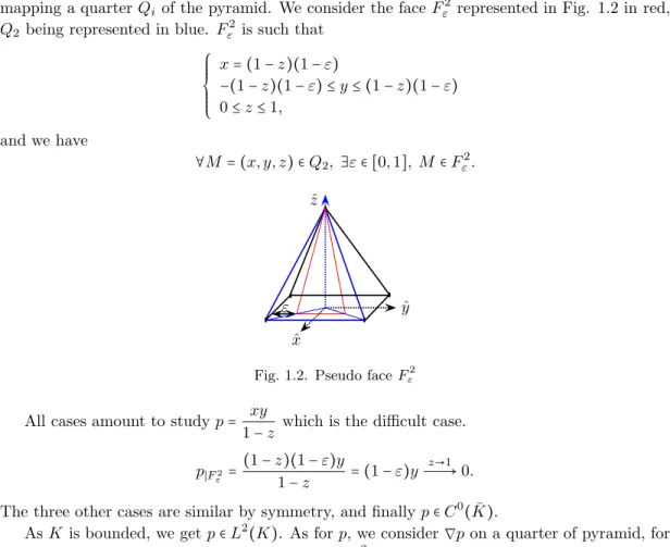
mapping a quarter Qi of the pyramid. We consider the face F 2

ε represented in Fig. 1.2 in red,

Q2 being represented in blue. F_ε2is such that

⎧⎪⎪⎪⎪ ⎨⎪⎪⎪ ⎪⎩ x= (1 − z)(1 − ε) −(1 − z)(1 − ε) ≤ y ≤ (1 − z)(1 − ε) 0≤ z ≤ 1, and we have ∀M = (x,y,z) ∈ Q2, ∃ε ∈ [0,1], M ∈ F_ε2. ˆ x ˆ y ˆ z ε

Fig. 1.2. Pseudo face Fε2

All cases amount to study p= xy

1− z which is the difficult case. p∣F2 ε = ( 1− z)(1 − ε)y 1− z = (1 − ε)y z→1 ÐÐ→ 0. The three other cases are similar by symmetry, and finally p∈ C0( ¯K).

As K is bounded, we get p∈ L2(K). As for p, we consider ∇p on a quarter of pyramid, for example Q2 and we consider an ε such that M∈ F

2 ε, and −(1 − ε)2 ≤∂p_∂z ∣F2 ε ≤ (1 − ε)2 ,

that is ∂zpis bounded. The same technique applied for ∂xpand ∂ypleads to conclude that∇p

Proposition 1.6 ensures to a function u∈ Vh to be continuous across the interface between

elements, whatever the type of the elements adjacent to the face, and therefore to belong to H1(Ω) due to proposition 1.7.

Proposition 1.8 The optimal finite element space of order r on the unit cube ̃Qis Cr= ˆPr○ T = ∑

0≤k≤r

Qk(̃x, ̃y)(1 − ̃z)k.

Proof. Using the transformation T, the polynomial part of ˆPrbecomes

{ˆxm_yˆn_ˆzp_{, m+ n + p ≤ r} ○ T = {(1 − 2̃x)}m_{(1 − 2̃y)}n_{(1 − ̃z)}m+n_̃zp_{, m+ n + p ≤ r}}

= {̃xm_̃yn_̃zp_{(1 − ̃z)}m+n

, m+ n + p ≤ r} ⊂ Cr,

whereas the fractional part of ˆPr becomes

{ˆxi_yˆj₍ xˆˆy

1− ˆz)

r−p

, i+ j ≤ p ≤ r − 1} ○ T = {(2̃x− 1)r−p+i(2̃y− 1)r−p+j(1 − ̃z)r−p+i+j, i+ j ≤ p ≤ r − 1} = {̃xr−k+i_̃yr−k+j_{(1 − ̃z)}r−k+i+j_{,0≤ i + j ≤ k ≤ r − 1} ⊂ C}

r,

that is ̃Pr⊂ Cr.

We now notice that dim Cr= ∑

0≤k≤r(k + 1) 2

= 1₆(r + 1)(r + 2)(2r + 3) = dim ˆPr= dim ̃Pr,

which proves the proposition. ◻

1.3. Location of the Degrees of Freedom

We wish to link continuously pyramidal elements with other elements of the mesh

ˆ hexahedra with Legendre-Gauss-Lobatto (LGL) points ;

ˆ tetrahedra with Hesthaven “electrostatic points” constructed with LGL points on edges

(Hesthaven and Teng[20]);

ˆ wedges obtained by a tensorial product of a face of a tetrahedron of Hesthaven, that is a

triangle of Hesthaven (Hesthaven [19]), with an edge with LGL points.

We place the degrees of freedom on LGL points on the quadrangular base of the pyramid, and on Hesthaven points on each triangular face. The number of degrees of freedom nf on the faces

is then

nf = 3r 2

+ 2. We add ni degrees of freedom inside the pyramid

ni=

1

6(r − 1)(r − 2)(2r − 3) = ∑1≤k≤r−2

k2.

Fig. 1.3. Location of the degrees of freedom inside the pyramidal element of order 5 The total number of degrees of freedom is

nr= ni+ nf=

1

6(r + 1)(r + 2)(2r + 3). which is precisely the dimension of ˆPr.

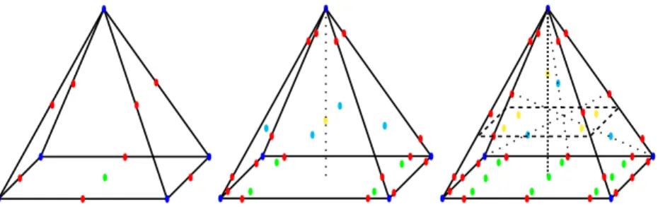
Degrees of freedom can then be placed systematically on the pyramid, at any order. Each category of point is represented by a color in the Fig. 1.4 for the pyramidal elements of order two to four.

Fig. 1.4. Location of the degrees of freedom for the pyramidal elements of order 2, 3 and 4 (Color online)

1.4. Basis Functions

The basis functions on the reference pyramid ˆK are obtained by inverting a Vandermonde system as follow.

Let ( ˆMi)1≤i≤nr the locations of the interpolation points on the pyramid, and( ˆψi)1≤i≤nr a

base of ˆPr,

Definition 1.9 The Vandermonde matrix V DM∈ Mnr(R) is defined by

V DMi,j= ˆψi( ˆMj), 1 ≤ i,j ≤ nr, (8)

and the basis function ˆϕi linked to the interpolation point ˆMi is then defined as

ˆ

ϕi= ∑

1≤j≤nr

(V DM−1₎

Proposition 1.10 The following set of basis functions is an orthogonal base of ˆPr {P0,0 i ( ˆ x 1− ˆz)P 0,0 j ( ˆ y 1− ˆz) (1− ˆz) max(i,j)

P_k2max(i,j)+2,0(2ˆz− 1), 0 ≤ i,j ≤ r, 0 ≤ k ≤ r − max(i,j)} , where Pmi,j(x) denotes the Jacobi polynomial of order m, orthogonal for the weight (1−x)i(1+x)j.

Proof. We note ˆ ψi,j,k(ˆx, ˆy, ˆz) = P_i0,0( ˆ x 1− ˆz)P 0,0 j ( ˆ y 1− ˆz) (1− ˆz) max(i,j) P_k2max(i,j)+2,0(2ˆz− 1). We first prove that the family is orthogonal by using the transformation (2) on ˜Qr

∫_Kˆψˆi,j,k(ˆx, ˆy, ˆz) ˆψi′,j′,k′(ˆx, ˆy, ˆz) dˆx dˆydˆz =

∫ 1 0 P 0,0 i (2̃x− 1)P 0,0 i′ (2̃x− 1) d̃x ´¹¹¹¹¹¹¹¹¹¹¹¹¹¹¹¹¹¹¹¹¹¹¹¹¹¹¹¹¹¹¹¹¹¹¹¹¹¹¹¹¹¹¹¹¹¹¹¹¹¹¹¹¹¹¹¹¹¹¹¹¹¹¹¹¹¹¹¹¹¹¹¹¹¹¹¹¹¹¹¹¹¹¹¹¹¹¹¹¹¹¹¹¹¹¹¹¹¹¹¹¹¹¹¹¹¹¸¹¹¹¹¹¹¹¹¹¹¹¹¹¹¹¹¹¹¹¹¹¹¹¹¹¹¹¹¹¹¹¹¹¹¹¹¹¹¹¹¹¹¹¹¹¹¹¹¹¹¹¹¹¹¹¹¹¹¹¹¹¹¹¹¹¹¹¹¹¹¹¹¹¹¹¹¹¹¹¹¹¹¹¹¹¹¹¹¹¹¹¹¹¹¹¹¹¹¹¹¹¹¹¹¹¶ = Cii′δi i′ ∫ 1 0 P 0,0 j (2̃y− 1)P 0,0 j′ (2̃y− 1) d̃y ´¹¹¹¹¹¹¹¹¹¹¹¹¹¹¹¹¹¹¹¹¹¹¹¹¹¹¹¹¹¹¹¹¹¹¹¹¹¹¹¹¹¹¹¹¹¹¹¹¹¹¹¹¹¹¹¹¹¹¹¹¹¹¹¹¹¹¹¹¹¹¹¹¹¹¹¹¹¹¹¹¹¹¹¹¹¹¹¹¹¹¹¹¹¹¹¹¹¹¹¹¹¹¹¹¹¸¹¹¹¹¹¹¹¹¹¹¹¹¹¹¹¹¹¹¹¹¹¹¹¹¹¹¹¹¹¹¹¹¹¹¹¹¹¹¹¹¹¹¹¹¹¹¹¹¹¹¹¹¹¹¹¹¹¹¹¹¹¹¹¹¹¹¹¹¹¹¹¹¹¹¹¹¹¹¹¹¹¹¹¹¹¹¹¹¹¹¹¹¹¹¹¹¹¹¹¹¹¹¹¹¶ = Cjj′δj j′ 4 _∫ 1 0 (1 − ̃z) max(i,j)+max(i′_,j′₎₊₂ P_k2max(i,j)+2,0(2̃z− 1)P_k2max(i′ ′,j′)+2,0(2̃z− 1) d̃z,

with 0≤ i,j ≤ r, 0 ≤ k ≤ r − max(i,j), and when i = i′and j= j′ ∫ 1 0 (1 − ̃z) 2max(i,j)+2 P_k2max(i,j)+2,0(2̃z− 1)P_k2max(i,j)+2,0′ (2̃z− 1) d̃z = Ckk′δk k′. We also have

{ ˆψi,j,k(ˆx, ˆy, ˆz), 0 ≤ i,j ≤ r, k ≤ r − max(i,j)} ○ T−1=

{P0,0 i (2̃x− 1)P 0,0 j (2̃y− 1)(1 − ̃z) max(i,j)_P2max(i,j)+2,0 k (2̃z− 1), 0 ≤ i,j ≤ r, k ≤ r − max(i,j)} ⊂ Cr,

that is, with an argument of dimension,

Span{ ˆψi,j,k(ˆx, ˆy, ˆz), 0 ≤ i,j ≤ r, k ≤ r − max(i,j)} ○ T−1= Cr,

which proves the proposition. ◻

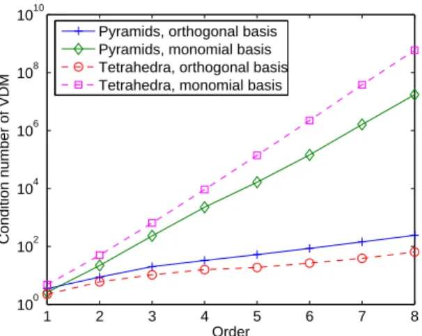
We compare the condition number of the Vandermonde matrix for monomial and orthogonal bases of ˆPr in the case of tetrahedral and pyramidal elements on Fig. 1.5. We notice that

the condition number of the Vandermonde matrix is increasing faster for tetrahedra than for pyramids when using monomial base, whereas we observe the opposite for orthogonal base. Besides, the use of the orthogonal set of basis functions highly improves the condition number of the VDM matrix.

Remark 1.11 The characterization of the invertibility of the Vandermonde matrix is an open question, but we observed that the VDM matrix is invertible with our choice of position for the degrees of freedom, the element is therefore unisolvent.

2. Comparison with Existing Methods

The nodal basis functions we propose are the same as Bedrosian [2], Zgainski et al. [33] and Chatzi and Preparata [6] for order one. They are identical to those of Graglia et al. [17] for order two, and they are new for order greater or equal to three.

The finite element space Cr of order r on the unit cube ̃Qdefined by in proposition 1.8 is

1 2 3 4 5 6 7 8 100 102 104 106 108 1010 Order Condition number of VDM

Pyramids, orthogonal basis Pyramids, monomial basis Tetrahedra, orthogonal basis Tetrahedra, monomial basis

Fig. 1.5. Condition number of the VDM matrix versus the order for tetrahedral and pyramidal elements, for monomial and orthogonal basis functions

Proposition 2.1 The subspace C_r0 of Cr with zero trace on the boundary of ̃Q is

C_r0(̃x, ̃y, ̃z) = (1 − ̃z)2̃x(1 − ̃x) ̃y(1 − ̃y) ̃z ̃Cr−3.

Proof. The basis functions obviously vanish on the boundary of ̃Qand belongs to Cr. The

dimension of the space is dim Cr−3=

1

6(r − 1)(r − 2)(2r − 3) = ni, which proves the proposition. ◻

We write transformation ¯T from the infinite pyramid ¯Qto the unit cube ̃Q.

¯ T ∶⎧⎪⎪⎪⎪⎪⎨ ⎪⎪⎪⎪⎪ ⎩ ̃x = ¯x ̃y = ¯y ̃z= ₁z_{+ ¯z}¯ . (10)

Proposition 2.2 The finite element space Ur proposed by Nigam and Phillips [24] on the

infinite pyramid ¯Q satisfies

Ur⊃ Cr○ ¯T,

and contains more degrees of freedom than Cr since

dim Ur= 1 + 3k + k 3

> dim Cr.

The subspace Ur0 of Ur whose trace is null on the boundary of the element is equal to

U_r0(¯x, ¯y, ¯z) = {x¯(1 − ¯x)¯y(1 − ¯y)¯z

(1 + ¯z)r u(¯x, ¯y, ¯z), u ∈ Q

r−2_{(¯x, ¯y, ¯z)} ,}

and if we replace U0r by C 0

r○ ¯T, we get the optimal space

¯

Ur= Cr○ ¯T.

Proof. Using the transformation (10), we detail the following basis functions (the others can be treated similarly by symmetry)

For the vertex : (1 − ¯x)(1 − ¯y) (1 + ¯z)r ○ ¯T

−1_{= (1 − ̃x)(1 − ̃y)(1 − ̃z)}r _{∈ C} r.

For the apex : z¯

r

(1 + ¯z)k ○ ¯T

−1_{= ̃z}r _{∈ C} r.

For the representative vertical edge : {(1− ¯x)(1 − ¯y)¯z_{(1 + ¯z)}r a, 1≤ a ≤ r − 2} ○ ¯T

−1_{= {(1 − ̃x)(1 − ̃y)(1 − ̃z)}r−a_̃za

,1≤ a ≤ r − 2} ⊂ Cr.

For the representative base edge : {(1− ¯x)(1 − ¯y)¯x_{(1 + ¯z)}r a, 1≤ a ≤ r − 2} ○ ¯T

−1_{= {(1 − ̃x)(1 − ̃y)̃x}a_{(1 − ̃z)}r_{, 1≤ a ≤ r − 2} ⊂ C} r.

For the representative triangular face : {(1− ¯x)(1 − ¯y)¯x

a_z¯b

(1 + ¯z)r , a, b≥ 0,a + b ≤ r − 1}○ ¯T −1₌

{(1 − ̃x)(1 − ̃y)̃xa_{(1 − ̃z)}r−b_̃zb

, 0≤ a + b ≤ r − 1} ⊂ Cr.

For the base face :

{(1− ¯x)(1 − ¯y)¯x_{(1 + ¯z)}r ay¯b, 1≤ a,b ≤ r − 1}○ ¯T

−1_{= {(1 − ̃x)(1 − ̃y)̃x}a_̃yb_{(1 − ̃z)}r_{, 1≤ a,b ≤ r − 1} ⊂}

Cr.

For the interior :

{x¯(1 − ¯x)¯y(1 − ¯y)¯z_{(1 + ¯z)}r u(¯x, ¯y, ¯z), u ∈ Q

r−2_{(¯x, ¯y, ¯z)} ○ ¯T}−1₌

{̃xi+1_{(1 − ̃x)̃y}j+1_{(1 − ̃y)̃z}k+1_{(1 − ̃z)}r−k

, 0≤ i,j,k ≤ r − 2} ⊃ Cr0.

The subspace of Urwhose trace is null on the boundary of the element is equal to

U_r0= {x¯(1 − ¯x)¯y(1 − ¯y)¯z (1 + ¯z)r u(¯x, ¯y, ¯z), u ∈ Q r−2_{(¯x, ¯y, ¯z)}} whose dimension is dim Ur0= dim Qr−2= (r − 1) 3 . Since there are nf = 3r

2

+ 2 basis functions associated with the boundary, we have dim Ur= 3r

2

+ 2 + (r − 1)3

= 1 + 3r + r3

> dim Cr.

If we replace U_r0by C_r0○ ¯T, the new finite element space ¯Ur satisfies

dim ¯Ur= dim Cr,

and

¯

Ur⊃ Cr○ ¯T,

that is we have the equality of these two spaces. ◻

We write transformation ÌT from the cube[−1,1]3 to the unit cube ̃Q

Ì T∶ ⎧⎪⎪⎪⎪ ⎪⎪⎪⎪ ⎨⎪⎪⎪ ⎪⎪⎪⎪⎪ ⎩ ̃x = 1+ a₂ ̃y =1+ b₂ ̃z =1+ c₂ . (11)

Proposition 2.3 The finite element space Wr of order r introduced by Warburton [30] on the

cube[−1,1]3 is not optimal.

The subspace of Wr whose trace is null on the boundary of the element is equal to

W_r0○ ÌT−1= {̃x(1 − ̃x)̃y(1 − ̃y)̃z(1 − ̃z)2u(̃x, ̃y, ̃z), u ∈ Pr−3(̃x, ̃y, ̃z)} .

If we replace W0r by C 0

r○ ÌT, and the basis functions linked to the base face by the following set

of functions

{(1− a₂ ) (1+ a₂ ) (1− b₂ ) (1+ b₂ ) (1− c₂ )max(i,j)+1P_i−11,1(a)P_j−11,1(b), 1 ≤ i,j ≤ r − 1}, we get the optimal space

Í

Wr= Cr○ ÌT .

Proof. Using the transformation (11), we detail the following basis functions (the others can be treated similarly by symmetry)

For the vertex : {(1− a

2 )( 1− b 2 ) ( 1− c 2 )} ○ ÌT −1_{= (1 − ̃x)(1 − ̃y)(1 − ̃z) ∈ C} r.

For the apex : {1+ c 2 } ○ ÌT

−1_{= ̃z ∈ C} r.

For the vertical edge : {(1− a 2 ) ( 1− b 2 ) ( 1− c 2 ) ( 1+ c 2 ) P 1,1 i−1(c), 1 ≤ i ≤ r − 1} ○ ÌT −1₌ {(1 − ̃x)(1 − ̃y)(1 − ̃z)̃zP1,1 i−1(2̃z− 1), 1 ≤ i ≤ r − 1} ⊂ Cr.

For the base edge :

{(1− a₂ ) (1+ a₂ ) (1− b₂ ) (1− c₂ )i+1P_i−11,1(a), 1 ≤ i ≤ r − 1} ○ ÌT−1= {̃x(1 − ̃x)(1 − ̃y)(1 − ̃z)i+1_P1,1

i−1(2̃x− 1), 1 ≤ i ≤ r − 1} ⊂ Cr.

For the base face :

{(1− a₂ ) (1+ a₂ ) (1− b₂ ) (1+ b₂ ) (1− c₂ )i+j+1P_i−11,1(a)P_j−11,1(b), 1 ≤ i,j ≤ r − 1} ○ ÌT−1= {̃x(1 − ̃x)̃y(1 − ̃y)(1 − ̃z)i+j+1

P_i−11,1(2̃x− 1)P_j−11,1(2̃y− 1), 1 ≤ i,j ≤ r − 1} ⊄ Cr. For the triangular face :

{(1− a 2 ) ( 1+ a 2 ) ( 1− b 2 ) ( 1− c 2 ) i+1 (1+ c 2 ) P 1,1 i−1(a)P 2i+1,1 j−1 (c), i + j ≤ r − 1,i,j ≥ 1} ○ ÌT −1₌ {(1 − ̃x)̃x(1 − ̃y)(1 − ̃z)i+1_̃zP1,1 i−1(2̃x− 1)P 2i+1,1 j−1 (2̃z− 1), i + j ≤ r − 1,i,j ≥ 1} ⊂ Cr.

For the interior :

{(1− a₂ ) (1+ a₂ ) (1− b₂ ) (1+ b₂ ) (1− c₂ )i+j+1(1+ c₂ ) P1,1 i−1(a)P 1,1 j−1(b)P 2i+2j+1,1 k−1 (c), i + j + k ≤ r − 1, i,j,k ≥ 1} ○ Ì

T−1= {̃x(1 − ̃x)̃y(1 − ̃y)̃z(1 − ̃z)i+j+1P_i−11,1(2̃x − 1)P_j−11,1(2̃y− 1)P_k−12i+2j+1,1(2̃z− 1), i + j + k ≤ r − 1, i,j,k ≥ 1} ⊂ Cr.

The subspace W_r0 of Wr whose trace is null on the boundary of the element is equal to

whose dimension is

dim W_r0= dim Pr−3= (

r− 2)(r − 1)r

6 .

Since there are 3r2+ 2 basis functions associated with the boundary, we have dim Wr= ( r− 2)(r − 1)r 6 + 3r 2 + 2 = (r+ 1)(r + 2)(r + 3)₆ + r2 < dim Cr.

If we replace the proposed set of basis functions for the base face by the following one {(1− a₂ ) (1+ a₂ ) (1− b₂ ) (1+ b₂ ) (1− c₂ )max(i,j)+1P_i−11,1(a)P_j−11,1(b), 1 ≤ i,j ≤ r − 1} ○ ÌT−1= {̃x(1 − ̃x)̃y(1 − ̃y)(1 − ̃z)max(i,j)+1_P1,1

i−1(2̃x− 1)P 1,1 j−1(2̃y− 1) 1 ≤ i,j ≤ r − 1} ⊂ Cr, and W0 r by C 0

r○ ÌT, the new finite element space ÍWr will satisfy

Í

Wr⊂ Cr○ ÌT

and

dim ÍWr= dim Cr,

that is we have the equality of the two spaces. ◻

Remark 2.4 As W1 = ÍW1 but Wr ⊅ ÍW2, using Wr as a finite element space for pyramidal

elements ensures not more than a first-order convergence in H1-norm.

Numerical study of the dispersion error has been conducted on periodic meshes containing non-affine pyramids in order to check these theoretical results (see Fig. 6.6 in section 6.3).

3. Quadrature Formula

To evaluate integrals, we use a quadrature rule defined over the reference pyramid ˆK. A simple rule consists in taking Gauss points over the unit cube ̃Q of coordinates(̃x, ̃y, ̃z), and compute their image on the reference pyramid ˆK of coordinates (ˆx, ˆy, ˆz), via the change of variable T defined by equation (2), which is a diffeomorphism from the open ̃Qto the open ˆK.

For any function f , we denote ̃

f(̃x, ̃y, ̃z) = ˆf(ˆx, ˆy, ˆz), and the change of variable provides

∫_Kˆfˆ(ˆx, ˆy, ˆz) dˆxdˆydˆz = ∫_Q̃4 ̃f(̃x, ̃y, ̃z) (1 − ̃z) 2

d̃xd̃yd̃z. (12)

Definition 3.1 Let M be the mass matrix for the pyramid K, defined by Mi,j= ∫

Kϕiϕjdxdydz= ∫Kˆ∣DF∣ ˆϕiϕˆjdˆxdydˆˆ z (13)

and K the stiffness matrix such that Ki,j= ∫ K∇ϕi ⋅ ∇ϕjdxdydz= ∫_ˆ K∣DF∣DF −1_DF∗−1_∇ˆϕˆ i⋅∇ˆϕˆjdˆxdydˆˆ z. (14)

Definition 3.2 We define the polynomial space

Q_m,n,p= {xiyjzk,0≤ i ≤ m,0 ≤ j ≤ n,0 ≤ k ≤ p}.

Lemma 3.3

∀i∈ J1,nrK, ̃ϕi∈ Qr(̃x, ̃y, ̃z).

Proof. Using proposition 1.8,̃ϕi(̃x, ̃y, ̃z) ∈ Cr(̃x, ̃y, ̃z), and we obviously have Cr⊂ Qr, which

proves the lemma. ◻

Lemma 3.4

∀i∈ J1,nrK, ˆ∇ϕ̃i∈ Qr−1,r,r−1×Qr,r−1,r−1×Qr,r,r−1(̃x, ̃y, ̃z).

Proof. We decompose ˆϕi(ˆx, ˆy, ˆz) into the monomial base ˆψj(ˆx, ˆy, ˆz) of ˆPr and we treat the

different cases.

We first consider the derivative in x, the derivative in y being treated similarly by symmetry: either ˆψj(ˆx, ˆy, ˆz) ∈ Pr(ˆx, ˆy, ˆz),

∂ ˆψj ∂xˆ (ˆx, ˆy, ˆz) = ˆx m−1_yˆn_zˆp_{= (2̃x− 1)}m−1_{(2̃y− 1)}n_{(1 − ̃z)}m+n−1_̃zp_{, m + n + p≤ r,} or ∂ ˆψj ∂xˆ (ˆx, ˆy, ˆz) = ˆ xr−p+i−1yˆr−p+j (1 − ˆz)r−p = (2̃x− 1)

r−p+i−1_{(2̃y− 1)}r−p+j_{(1 − ̃z)}r−p+i+j−1

, i + j≤ p ≤ r − 1,

that is ∂ ̃ψj

∂xˆ (̃x, ̃y, ̃z) ∈ Qr−1,r,r−1(̃x, ̃y, ̃z) in both cases. Similarly, for the derivative in z, either

∂ ˆψj ∂zˆ(ˆx, ˆy, ˆz) = ˆx m_yˆn_zˆp−1_{= (2̃x− 1)}m_{(2̃y− 1)}n_̃zp−1_{(1 − ̃z)}m+n_{, m + n + p≤ r} or ∂ ˆψj ∂zˆ (ˆx, ˆy, ˆz) = ˆ xr−p+iyˆr−p+j (1 − ˆz)r−p+1 = (2̃x− 1)

r−p+i_{(2̃y− 1)}r−p+j_{(1 − ̃z)}r−p+i+j−1_{, i + j≤ p ≤ r − 1,}

that is ∂ ̃ψj

∂zˆ (̃x, ̃y, ̃z) ∈ Qr,r,r−1(̃x, ̃y, ̃z) in both cases. ◻

Lemma 3.5 ̃ DF = (∂ ̃F ∂xˆ, ∂ ̃F ∂yˆ, ∂ ̃F ∂zˆ) ∈ Q 3 0,1,0×Q 3 1,0,0×Q 3 1,1,0(̃x, ̃y, ̃z), and ̃ ∣DF∣ ∈ Q1,1,0(̃x, ̃y, ̃z).

Proof. The derivatives of F can be written as ∂F ∂xˆ = 1 4(−S1+S2+S3−S4) + 1 4(S1−S2+S3−S4) ˆ y 1 − ˆz = 1 4(−S1+S2+S3−S4) + 1 4(S1−S2+S3−S4)(2̃y− 1) = A1+C̃y, ∂F ∂ˆy = 1 4(−S1−S2+S3+S4) + 1 4(S1−S2+S3−S4) ˆ x 1 − ˆz = 1 4(−S1−S2+S3+S4) + 1 4(S1−S2+S3−S4)(2̃x− 1) = A2+C̃x, ∂F ∂ˆz = 1 4(4S5−S1−S2−S3−S4) + 1 4(S1−S2+S3−S4) ˆ xˆy (1 − ˆz)2 = 1₄(4S5−S1−S2−S3−S4) +1 4(S1−S2+S3−S4)(2̃x − 1)(2̃y− 1) = A3+2C̃x̃y.

The determinant is then ̃

∣DF∣(̃x, ̃y, ̃z) = det(A1+C̃y,A2+C̃x,A3+2C̃x̃y).

We can develop the expression in ̃

∣DF∣(̃x, ̃y, ̃z) = det(A1, A2, A3) + ̃x det(A1, C, A3) + ̃y det(C,A2, A3) + 2 ̃x̃y det(A1, A2, C),

which proves the lemma. ◻

Proposition 3.6 When F is affine, the quadrature formula must be exact for polynomials of (1 − z)2

Q2r for the mass matrix and(1 − z)2Q2r,2r,2r−2 for the stiffness matrix, such that these

matrices are exactly integrated.

When F is not affine, for the mass matrix to be exactly integrated, the quadrature formula must be exact for polynomials of(1 − z)2Q2r+1,2r+1,2r.

Proof. In the affine case, we can factorize the mass matrix by coefficient ∣DF∣ which is constant. For the mass matrix, the lemma 3.3 provides the term̃ϕĩϕj(1−̃z)

2

to be in(1−̃z)2Q2r.

For the stiffness matrix, thanks to lemma 3.4, the term∂̃ϕi ∂̃x ∂̃ϕj ∂̃x (1−̃z) 2 is in(1−̃z)2Q2r−2,2r,2r−2, the term ∂̃ϕi ∂̃y ∂̃ϕj ∂̃y (1 −̃z) 2

is in (1 − ̃z)2Q2r,2r−2,2r−2 and the term

∂̃ϕi ∂̃z ∂̃ϕj ∂̃z (1 −̃z) 2 is in (1 − ̃z)2

Q2r,2r,2r−2, that is the final term is in(1 − ̃z) 2

Q2r,2r,2r−2.

In the non-affine case, using the result of the affine case and lemma 3.5, we can easily conclude that we need a quadrature rule exact for polynomials of(1−̃z)2Q2r+1,2r+1,2rto exactly

integrate the mass matrix. ◻

Remark 3.7 Because of the rational fraction due to ̃DF−1, the stiffness matrix can not be exactly integrated with a classical quadrature formula.

To integrate exactly the mass matrix, we choose the following quadrature formula : (ξG

where (ξ_iG, ωG_i ) is the classical Gauss quadrature rule, exact for polynomials of Q2r+1, and

(ωHM

k , ξkHM) a Gauss-Jacobi rule for the evaluation of ∫ (1 − x) 2

f(x), exact for polynomials of (1 − x)2Q2r+1. For this last rule, quadrature points and weights have been calculated in

Hammer, Marlowe and Stroud [18]. Eventually, we need(r +1)3integration points for an exact integration of the mass matrix.

4. Error Estimates

4.1. Functional Spaces and Basic Notations Let Ω be an open set of R3.

Definition 4.1 We define L2(Ω) = {u ∈ L2_loc∣ ∫ Ω∣u∣ 2 < +∞} Hm(Ω) = {u ∈ L2(Ω) ∣ ∂ α u ∂xα ∈ L 2 (Ω),∣α∣ ≤ m} equipped with the usual norm in Hm(Ω)

∣∣u∣∣2

m,Ω= ∑ ∣α∣≤m∫Ω

∣∂_∂xαuα∣ 2

and the usual semi-norm in Hm_(Ω)

∣u∣2 m,Ω= ∑ ∣α∣=m∫Ω ∣∂_∂xαuα∣ 2 . We obviously have the inequality

∀u∈ Hm(Ω), ∣u∣2_m,Ω≤ ∣∣u∣∣2_m,Ω. (15)

An approximate integral using a Gauss-type quadrature formula is denoted _∮

G

, and πr

will denote a projector on the polynomial space Pr.

4.2. Presentation of the Problem

We consider a standard variational problem

{ Find u_{∀v∈ V, a(u,v) = f(v),}∈ V such that (16) where the space V = H1(Ω), a(.,.) a continuous bilinear and coercive form, and f(.) a con-tinuous linear form. Then, given a finite-dimensional subspace Vh of the space V , the discrete

problem reads

{ Find uh∈ Vh such that

∀vh∈ Vh, ah(uh, vh) = fh(vh),

(17) where ah(.,.) is a bilinear form defined over the space Vh, uniformly Vh-elliptic, and fh(.) is a

linear form defined over the space Vh.

We shall consider the simple case where a(u,v) = ∫

Ωuv +∫Ω

4.3. Abstract Error Estimate

We will consider the following version of Strang’s lemma

Lemma 4.2 (Strang’s lemma). If u is the solution of (16) and uh the solution of (17), there

exists a constant C> 0 which does not depend on the space step h such that ∥u − uh∥1≤ C inf vh∈Vhr { ∥u − vh∥1 ´¹¹¹¹¹¹¹¹¹¹¹¹¹¹¹¹¹¹¹¹¹¹¹¹¹¹¹¹¹¹¹¹¹¹¹¹¹¹¹¹¹¹¹¹¸¹¹¹¹¹¹¹¹¹¹¹¹¹¹¹¹¹¹¹¹¹¹¹¹¹¹¹¹¹¹¹¹¹¹¹¹¹¹¹¹¹¹¹¹¶ interpolation error + _sup wh∈Vhr ∣a(vh, wh) − ah(vh, wh)∣ ∥wh∥1

´¹¹¹¹¹¹¹¹¹¹¹¹¹¹¹¹¹¹¹¹¹¹¹¹¹¹¹¹¹¹¹¹¹¹¹¹¹¹¹¹¹¹¹¹¹¹¹¹¹¹¹¹¹¹¹¹¹¹¹¹¹¹¹¹¹¹¹¹¹¹¹¹¹¹¹¹¹¹¹¹¹¹¹¹¹¹¹¹¹¹¹¹¹¹¹¹¹¹¸¹¹¹¹¹¹¹¹¹¹¹¹¹¹¹¹¹¹¹¹¹¹¹¹¹¹¹¹¹¹¹¹¹¹¹¹¹¹¹¹¹¹¹¹¹¹¹¹¹¹¹¹¹¹¹¹¹¹¹¹¹¹¹¹¹¹¹¹¹¹¹¹¹¹¹¹¹¹¹¹¹¹¹¹¹¹¹¹¹¹¹¹¹¹¹¹¹¶_{numerical integration error} }.

Proof. The proof of this version of Strang’s lemma is similar to the proof proposed by Ciarlet

[7] for his version, noticing that, in our case, Vh⊂ V . ◻

We now study separately the two terms of the right hand-side of the Strang’s lemma, namely the interpolation error and the quadrature error. As Pr⊂ PrF, we first consider the case

of vh= πruh∈ Prand get estimates in this case, and we will then take the infimum for vh∈ PrF

to get Strang’s lemma. We also suppose that u is in Hr+1(Ω) for an Ω regular enough. 4.3.1. Interpolation error

Let Ω a set composed of n pyramids Ki

Ω= ⋃ 1≤i≤n Ki. We denote hKi= diam (Ki) = sup x,y∈Ki ∣x − y∣, h = sup 1≤i≤n hKi.

Let us recall the Bramble-Hilbert’s lemma (Ciarlet [7])

Lemma 4.3 (Bramble-Hilbert’s lemma). Let r≥ 1, m ≤ r + 1. We denote by πr the projector

to Pr satisfying

∀p∈ Pr(K), πrp= p.

Then, there exists a constant CK> 0 which only depends on K and r such that

∀_u∈ Hr+1(K), ∥u − π_ru∥

m,K ≤ CKhr+1−mK ∣u∣r+1,K.

We consider a domain made of a single pyramid K, (Ω= K). For u in Hr+1(Ω), we apply Bramble-Hilbert lemma

∣∣u − πru∣∣m,K≤ CKhKr+1−m∣u∣r+1,K,

where CK depends on the shape of the pyramid K.

We suppose that the constants CKi for each element Ki of Ω are bounded by a constant C,

∀Ki∈ Ω, CKi≤ C. (18)

For m= 1, the sum for all the elements Ki of Ω and the inequality (15) on norms give the error

estimates on Ω

∥u − πru∥1,Ω≤ Ch r_{∣∣u∣∣}

r+1,Ω. (19)

Remark 4.4 The condition CK≤ C is satisfied in the case of periodic meshes of the following

sections, since the number of pyramids of different shape is finite. In a more general case, we conjecture that the boundedness of CK is related to the existence of an upper bound for the

4.3.2. Quadrature Error

We now seek the minimal integration formula in order to obtain a quadrature error of order r. Definition 4.5 For(vh, wh) ∈ PrF and K∈ Ω, we denote

EK(vh, wh) = ∫

Kvhwhdxdydz −∮Kvhwhdxdydz,

where the approximate integral_∮

Kvhwhdxdydz is exact for(1 − z) 2

Q_m,m,n.

We first get estimates for the mass term of the bilinear form a. Lemma 4.6 ∀(vh, wh) ∈ PrF, K∈ Ω and 0 ≤ p,q ≤ m − r − 1, we have

EK(vh, wh) = EK(vh−πpvh, wh−πqwh)

for a quadrature formula exact for polynomials of(1 − z)2Qm,m,m−1

Proof. Let us consider the integral

∫_Kπpvhwhdxdydz.

After change of variable, we get

∫_Q̃4(1 − ̃z) 2

(πp̃vh)(̃∣DF∣ ̃wh) d̃xd̃yd̃z.

For a quadrature rule exact for polynomials of(1−z)2Qm,m,m−1, as πp̃vh∣DF∣ ̃̃wh∈ Qp+r+1,p+r+1,p+r(̃x, ̃y, ̃z),

we have

EK(πpvh, wh) = 0, (20)

for r + p + 1≤ m, that is p ≤ m − r − 1, using lemma 3.3. Similarly, we have

EK(vh, πqwh) = 0

for q≤ m − r − 1, and for p,q ≤ m − r − 1, we check that EK(πpvh, πqwh) = 0,

which provides the claimed result. ◻

Proposition 4.7 For K∈ Ω and vh∈ Pr(K),

sup wh∈PrF E(vh, wh) ∣∣wh∣∣1,K ≤ C ′ KhrK∣∣vh∣∣r,K

Proof. We apply lemma 4.6 for p= r − 2 and q = 0

E(vh, wh) = E(vh−πr−2vh, wh−π0w_h).

Using the Cauchy-Schwarz inequality for both the exact and the approximate integral, which is possible since the norm defined by approximate integration is equivalent to the usual norm with a constant CN, we get

∣E(vh, wh)∣ ≤ CN∣∣vh−πr−2vh∣∣0,K∣∣wh−π0wh∣∣0,K.

As vh∈ Pr(K) ⊂ Hr(K) and wh∈ H 1

(K), Bramble-Hilbert’s lemma and the inequality on the norms (15) provides

∣∣vh−πr−2vh∣∣0,K≤ CKhr−1K ∣∣vh∣∣r,K.

∣∣wh−π0w_h∣∣0,K≤ CKhK∣∣wh∣∣1,K.

Hence

∣E(vh, wh)∣ ≤ CK′ hKr∣∣vh∣∣r,K∣∣wh∣∣1,K

with C_K′ = CNCK independent of wh. Therefore, we obtain the claimed result. ◻

We then find estimates for the stiffness term of a. Lemma 4.8

((1 − ̃z)2̃

∣DF∣̃DF∗−1∇̃ϕ_i) (̃x, ̃y, ̃z) ∈ (1 − ̃z)2Qr,r+1,r−1×Qr+1,r,r−1×Qr+1,r+1,r−1(̃x, ̃y, ̃z).

Proof. As ̃∣DF∣̃DF∗−1 is the comatrix of ̃DF, using lemma 3.5, we get ̃ ∣DF∣̃DF∗−1 = (A2∧A3, −A1∧A3, A1∧A2) +(C ∧ A3,0, A1∧C) ̃x + (0,−C ∧ A3, C ∧ A2) ̃y +₂(A2∧C, −A1∧C,0) ̃x̃y that is ̃ ∣DF∣̃DF∗−1∈ Q1,1,0(̃x, ̃y, ̃z) 3 . As (∇̃ϕi)(̃x, ̃y, ̃z) ∈ Qr−1,r,r−1×Qr,r−1,r−1×Qr,r,r−1(̃x, ̃y, ̃z),

by summing degrees, we obtain the claimed result. ◻

Lemma 4.9 ∀(vh, wh) ∈ PrF, K∈ Ω and 0 ≤ p ≤ m − r − 1, we have

EK(∇vh, ∇wh) = EK(∇vh−πp∇vh, ∇wh)

for a quadrature formula exact for polynomials of(1 − z)2Qm,m,m−2

Proof. As for lemma 4.6, we prove that

EK(πp∇vh, ∇wh) = 0

by considering the integral

After the change of variable, we get ∫_Q̃4(1 − ̃z) 2 (πp∇̃vh) ⋅ (̃∣DF∣̃DF ∗−1 ∇_w̃_h) d̃xd̃yd̃z.

For a quadrature rule exact for polynomials of(1−z)2Qm,m,m−2, using lemma 4.8,(πp∇̃vh)⋅

(̃∣DF∣̃DF∗−1∇w̃h) ∈ Qp+r+1,p+r+1,p+r−1(̃x, ̃y, ̃z), that is EK(πp∇vh, ∇wh) is equal to zero if r +

p +1≤ m, i.e. p ≤ m − r − 1. ◻

Proposition 4.10 For K∈ Ω and vh∈ Pr(K),

∀_wh∈ PF

r , EK(∇vh, ∇wh) = 0

for a quadrature formula exact for polynomials of(1 − z)2Qm,m,m−2, with m≥ 2r.

Proof. For vh ∈ Pr(K), that is ∇vh ∈ (Pr−1(K)) 3

, we apply lemma 4.9 with p = r − 1 to

conclude. ◻

We can now get the final quadrature error estimate using propositions 4.7 and 4.10, by summing for all the elements K of Ω and using (18)

sup wh∈Vhr ∣(a − ah)(vh, wh)∣ ∣∣wh∣∣1,Ω ≤ C ′_hr_∣∣v h∣∣r+1,Ω, vh∈ Pr(Ω) (21) with C′= CNC.

Theorem 4.11 For a quadrature formula which is exact for polynomials of(1 − z)2Qm,m,m−2,

for m≥ 2r, the final estimate from Strang’s lemma is inf vh∈V_hr ⎛ ⎝∣∣u − vh∣∣1,Ω+ sup wh∈V_hr ∣(a − ah)(vh, wh)∣ ∣∣wh∣∣1,Ω ⎞ ⎠≤ max(C,C′)hr∣∣u∣∣r+1,Ω.

Proof. Summing equations (19) and (21) with vh= πru, we get

∣∣u − πru∣∣1,Ω+ sup wh∈Vhr ∣(a − ah)(πru, wh)∣ ∣∣wh∣∣1,Ω ≤ C ′ hr∣∣πru∣∣r,Ω+Chr∣∣u∣∣r+1,Ω, vh∈ Pr(Ω).

We then use the inequality ∣∣πru∣∣m,Ω ≤ ∣∣u∣∣m,Ω to upper bound the right-hand side of the

inequality with max(C,C′), and we take the infimum for the left-hand side thanks to inclusion

(3). ◻

Remark 4.12 We can take the points and weights of quadrature (ξ_kG, ωG_k) to get a quadrature formula exact for Q2r+1, instead of (ξkHM, ωHMk ) in the previous quadrature formula, without

5. Discontinuous Galerkin Method

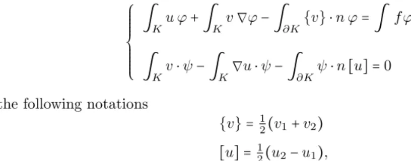
For any element K of boundary ∂K, we consider the Local Discontinuous Galerkin (LDG) formulation (Castillo et al. [5])

⎧⎪⎪⎪⎪ ⎪⎪ ⎨⎪⎪⎪ ⎪⎪⎪⎩ ∫_Ku ϕ +_∫ Kv ∇ϕ −∫∂K{v} ⋅ n ϕ = ∫ fϕ ∫_Kv ⋅ ψ −_∫ K ∇u ⋅ ψ −_∫ ∂Kψ ⋅ n[u] = 0

with the following notations

{v} =1

2(v1+v2)

[u] = 1

2(u2−u1),

where u1 is the value of u restricted to K, and u2 the value of u restricted to an element

adjacent to K.

We can take the space ˆPr identical to the one in the continuous case. The error estimates

are quite different from the ones obtained for continuous elements as the norm used for DG formulations is the L2norm, instead of the H1 norm.

6. Numerical Results

6.1. Dispersion

In order to study the pyramidal elements, a dispersion analysis is performed on the wave equation, relying on the computation of the phase error on infinite periodic meshes, as in Cohen [9]. The periodic cell is a cube that can be composed of a single hexahedron; of two wedges; of two pyramids and two tetrahedra (hybrid); or of six pyramids; or of six tetrahedra as shown in Fig. 6.1. The analysis has also been carried out on periodic cells made up of distorted cubes in order to check the consistency of our method when the base of the pyramid is not a parallelogram as shown in Fig. 6.2 for the hybrid cell.

Fig. 6.1. Cells for the regular periodic mesh : wedges (top-left), hybrid(top-right), pyramids (bottom-left) and tetrahedra (bottom-right)

Considering the Helmholtz equation

−ω2u −∆u= 0,

we look for plane solutions of the form u= e(ı⃗k⋅⃗x), where ⃗kis the wave vector, and∣∣⃗k∣∣ the wave number. The computational domain is reduced to a periodic cell where quasi-periodic conditions

Fig. 6.2. Periodic pattern for the hybrid case, with distorted pyramids (purple) and tetrahedra (gray) (Color online)

are enforced, so that the plane wave is a solution of the continuous equations problem. The numerical eigenvalue closest to the wave number∣∣⃗k∣∣ is denoted by ωh, so that we define qh as

qh=

ωh

∣∣⃗k∣∣. Since qhshould be close to 1, we can write

qh= 1 + C hp+o(hp)

where p denotes the dispersion order of the scheme.

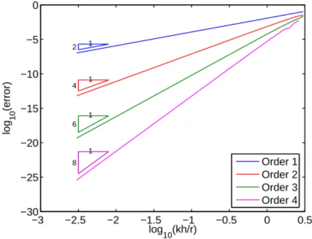
A dispersion order of 2r is obtained for both continuous and discontinuous Galerkin method, for regular as well as for distorted meshes (see Babuska and Osborn [1] for the factor 2), which coincides with the theoretical error estimates results obtained. This order of dispersion is clearly shown on the log-log curves in Fig. 6.3 for the continuous hybrid elements on a distorted mesh.

−3 −2.5 −2 −1.5 −1 −0.5 0 0.5 −30 −25 −20 −15 −10 −5 0 log 10(kh/r) log 10 (error) 1 2 1 4 1 6 1 8 Order 1 Order 2 Order 3 Order 4

Fig. 6.3. log-log dispersion error for continuous finite elements of orders 1 to 4 for a hybrid distorted mesh

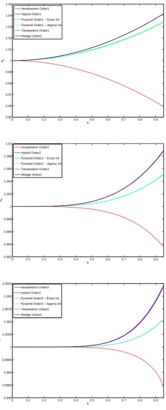
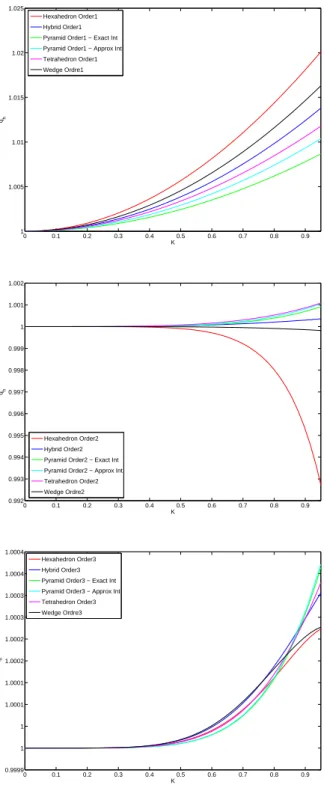
Dispersion curves are shown for regular elements of orders one to three in Fig. 6.4 for the continuous elements, and in Fig. 6.5 for the discontinuous elements. For the pyramids, exact and approximate integrations are giving very close results, and all elements exhibit similar

dispersion properties. The less dispersive element is the pyramidal one in most of the cases. The same study has been performed for distorted meshes and leads to the same conclusion. 6.2. Stability

The stability condition of the standard leap frog scheme is also computed on a periodic infinite mesh.

The CFL number, for which we have the stability condition ∆t≤ CFL h, is defined by

CF L= √ 1

max

∣∣⃗k∣∣≤π

λ(M−1(⃗k)K(⃗k))

,

where M(⃗k) and K(⃗k) are the mass and stiffness matrices associated with the periodic cell, and ⃗kthe wave vector.

For each type of element, the CFL number is given in Table 6.1 in the continuous case in Table 6.1, and in the discontinuous case in 6.2, up to order four. The stability criteria have been tested in the instationary case to check the correctness of the results.

Table 6.1: CFL for continuous finite elements with regular meshes.

Order 1 Order 2 Order 3 Order 4

Hexahedron 0.28868 0.11785 0.06697 0.04264 Wedge 0.15794 0.07176 0.04344 0.02926 Pyramid ExactInt 0.09682 0.04803 0.03083 0.02143 Pyramid ApproxInt 0.07217 0.03335 0.01985 0.01316 Tetrahedron 0.12247 0.06253 0.03919 0.02669 Hybrid 0.15138 0.07245 0.04558 0.03191

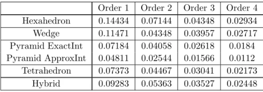
Table 6.2: CFL for discontinuous Galerkin method with regular meshes.

Order 1 Order 2 Order 3 Order 4

Hexahedron 0.14434 0.07144 0.04348 0.02934 Wedge 0.11471 0.04348 0.03957 0.02717 Pyramid ExactInt 0.07184 0.04058 0.02618 0.0184 Pyramid ApproxInt 0.04811 0.02544 0.01566 0.0112 Tetrahedron 0.07373 0.04467 0.03041 0.02173 Hybrid 0.09283 0.05363 0.03527 0.02448

For pyramidal elements, the CFL are computed with the quadrature formula(ξkHM, ωHMk )

presented in paragraph 4.3.2 for exact integration, and with Gauss quadrature formula(ξG k, ωkG)

for approximate integration. The CFL of pyramidal elements are clearly lower for approximate integrals (60% lower on average) than for exact integrals. In this case, the CFL of pyramidal elements is close to the tetrahedral’s.

0 0.1 0.2 0.3 0.4 0.5 0.6 0.7 0.8 0.9 0.95 0.96 0.97 0.98 0.99 1 1.01 1.02 1.03 1.04 1.05 K qh Hexahedron Order1 Hybrid Order1 Pyramid Order1 − Exact Int Pyramid Order1 − Approx Int Tetrahedron Order1 Wedge Ordre1 0 0.1 0.2 0.3 0.4 0.5 0.6 0.7 0.8 0.9 0.992 0.994 0.996 0.998 1 1.002 1.004 1.006 1.008 1.01 K qh Hexahedron Order2 Hybrid Order2 Pyramid Order2 − Exact Int Pyramid Order2 − Approx Int Tetrahedron Order2 Wedge Ordre2 0 0.1 0.2 0.3 0.4 0.5 0.6 0.7 0.8 0.9 0.998 0.9985 0.999 0.9995 1 1.0005 1.001 1.0015 1.002 1.0025 K qh Hexahedron Order3 Hybrid Order3 Pyramid Order3 − Exact Int Pyramid Order3 − Approx Int Tetrahedron Order3 Wedge Ordre3

0 0.1 0.2 0.3 0.4 0.5 0.6 0.7 0.8 0.9 1 1.005 1.01 1.015 1.02 1.025 K qh Hexahedron Order1 Hybrid Order1 Pyramid Order1 − Exact Int Pyramid Order1 − Approx Int Tetrahedron Order1 Wedge Ordre1 0 0.1 0.2 0.3 0.4 0.5 0.6 0.7 0.8 0.9 0.992 0.993 0.994 0.995 0.996 0.997 0.998 0.999 1 1.001 1.002 K qh Hexahedron Order2 Hybrid Order2 Pyramid Order2 − Exact Int Pyramid Order2 − Approx Int Tetrahedron Order2 Wedge Ordre2 0 0.1 0.2 0.3 0.4 0.5 0.6 0.7 0.8 0.9 0.9999 1 1 1.0001 1.0001 1.0002 1.0002 1.0003 1.0003 1.0004 1.0004 K qh Hexahedron Order3 Hybrid Order3 Pyramid Order3 − Exact Int Pyramid Order3 − Approx Int Tetrahedron Order3 Wedge Ordre3

Fig. 6.5. Dispersion curves for discontinuous Galerkin method of orders 1 to 3 for regular meshes (K = 6_{2πr )}kh

The same study has been performed for distorted meshes and leads to the same results, the CFL being smaller for the distorted meshes, and the CFL finally ranks as follows, in all the cases

CF LHexa> CFLW edge> CFLT etra> CFLP yr−ExactInt> CFLP yr−ApproxInt.

The CFL for a hybrid mesh is better than the tetrahedron’s and pyramid’s, which is a quite surprising result.

Remark 6.1 A study of optimal location for the degrees of freedom inside the pyramid has been performed to get an optimal CFL, but this location appears to have almost no influence on the CFL.

6.3. Numerical Comparison with Other Existing Methods

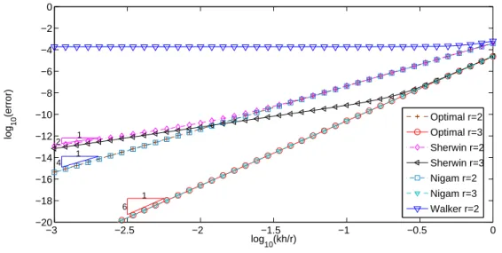
We display the dispersion obtained for the existing methods of Sherwin et al. [27], Nigam and Phillips [24], and Bluck and Walker [3] on Fig. 6.6, for order two and three. For order one, all these methods provide the same accuracy.

−3 −2.5 −2 −1.5 −1 −0.5 0 −20 −18 −16 −14 −12 −10 −8 −6 −4 −2 0 log 10(kh/r) log 10 (error) 1 2 1 4 1 6 Optimal r=2 Optimal r=3 Sherwin r=2 Sherwin r=3 Nigam r=2 Nigam r=3 Walker r=2

Fig. 6.6. Dispersion errors for the different types of existing elements of orders 2 and 3 with a distorted pyramidal mesh

The dispersion obtained with the space proposed by Sherwin et al. is of order two, whatever the order of approximation, as the basis functions for the base face and inside the pyramid are not sufficient to contain the optimal space. However, in the affine case, we check that we have a dispersion of order 2r.

The dispersion obtained for the optimal space is equal to the space proposed by Nigam and Phillips, that is the degrees of freedom they add are not necessary as they do not increase the accuracy.

For order two, the dispersion obtained by Bluck and Walker is not consistent (dispersion of order 0) because the space proposed does not contain the space of order one. However, in a case of an affine pyramid, the dispersion obtained is in h4 for order two.

6.4. Numerical Experiments 6.4.1. Test Case on a Cube

We first consider the Helmholtz equation on a cubic cavity with homogeneous Dirichlet bound-ary conditions

−ω2u −∆u = f(x,y,z), where

Ω = [−1,1]3 ω = 1.92 π,

and f is a Gaussian source centered at the origin. We study convergence on a hybrid mesh with a similar pattern as for the dispersion (see Fig. 6.2).

Displaying the L2 error obtained versus the space step h in a log-log scale in Fig. 6.7, we observe an L2error in O(hr+1) as proved in the error estimates. For these experiments, we used exact integration with r + 1 HM points in the direction ˜z and r + 1 Gauss points in directions ˜ xand ˜y. −1.3 −1.2 −1.1 −1 −0.9 −0.8 −0.7 −0.6 −0.5 −6 −5 −4 −3 −2 −1 0 log₁₀(h/r) log 10 (L2 error) 1 1 2 1 3 1 4 1 5 Order 1 Order 2 Order 3 Order 4

Fig. 6.7. L2 error versus h for the cubic cavity at different order of approximations.

6.4.2. Low Storage Matrix-Vector Product

Since the involved matrices can require a huge amount of memory, in particular for high order approximation like Q5, we use a low storage matrix vector product (i.e. a matrix-free

imple-mentation). This is quite classical in discontinuous Galerkin methods on hexahedra (Castel et al. [4]) or on tetrahedra (Hesthaven and Teng [20]), and the extension to pyramid and prismatic

elements is straightforward. For continuous formulation, we use similar techniques, i.e. that we exploit factorizations of elementary mass and stiffness matrix

∫ˆ K ∣DF∣ ˆϕi ˆ ϕj = ˆC DhCˆt ∫_Kˆ ∣DF∣DF −1 DF∗−1∇ˆϕ_ˆi⋅∇ˆϕˆj = ˆR BhRˆt, where matrices ˆ Ci,j = ˆϕi(ξj) ˆRi,j = ∇ ˆϕi(ξj)

are independent on the geometry, so they are not stored for each element, and matrices Dhand

Bh

(Dh)i,j = ωj∣DF∣(ξj)δi,j (Bh)i,j = ωj(∣DF∣DF −1

DF∗−1)(ξj)δi,j

are respectively diagonal and block-diagonal (each block being a symmetric 3x3 matrix). Such factorization is explained by Cohen and Fauqueux in [10], and shown to be very efficient for hexahedral elements, since ˆRis very sparse. In the case of other elements, ˆR is dense and does not induce any gain in computational time. Yet, we still use this factorization, since the storage induced is very low as we only store matrices Dhand Bh.

6.4.3. Test Case with Curved Isoparametric Elements on a Sphere Let us consider a sample test case of scattering by a sphere (see Fig 6.8)

⎧⎪⎪⎪⎪ ⎪⎪⎪⎪⎪ ⎨⎪⎪⎪ ⎪⎪⎪⎪⎪ ⎪⎩ −ω2u −∆u= 0 in Ω ∂u ∂n= − ∂uincident ∂n on Γ ∂u ∂n−iωu= 0 on Σ,

where Γ is a sphere of radius 3, ω= 2π, and Σ is the boundary of the cube [−5,5]3.

To have a good approximation of the geometry, curved isoparametric elements are used. The implementation of such elements is explained in ˇSol´ın et al. [28], except for pyramids for which the extension is straightforward. The reference solution is computed on a refined pure hexahedral mesh with Q7 elements. On Fig. 6.9, three different meshes used for third order

approximation are displayed.

The COCG solver (Clemens and Weiland [8]) is implemented, and can be used with or without preconditioning. In Table 6.3, the required number of degrees of freedom necessary to reach an error between one and two percent (measured in L2norm) are displayed for each type of mesh and at orders two, three and four. The results obtained without preconditioning and for a p-multigrid preconditioning using a damped Helmholtz equation (see Erlangga [15] for finite-difference, and Durufl´e [13] for finite element) are also displayed, along with the computational time. The order of the coarsest mesh is set to 1 for orders two and three, and set to 2 for order five and P4.

The performance of hybrid mesh is quite similar to a purely hexahedral mesh while purely tetrahedral meshes result in much more expensive computations. The last row of this table concerns the use of a Gauss-Seidel smoother instead of the Jacobi smoother used in other rows. Jacobi smoother fails for hybrid meshes, but we don’t have any explanation on this issue. In this case, a Q5approximation on hexahedral mesh is much faster than for tetrahedral elements.

Fig. 6.8. Real part of diffracted field for a sphere of radius 3 with Neumann condition.

Fig. 6.9. Meshes used for third order approximation. 6.4.4. Numerical Experiment on a Piano

We now perform computations using the discontinuous Galerkin method for the transient wave equation ⎧⎪⎪⎪⎪ ⎪⎪⎪⎪⎪ ⎨⎪⎪⎪ ⎪⎪⎪⎪⎪ ⎪⎩ ∂2u ∂t2 −∆u= f(x,t) in Ω ∂u ∂n = 0 on Γ ∂u ∂n+ ∂u ∂t = 0 on Σ, (22)

where Γ has the shape of the resonance cavity of a piano, and F is the surrounding parallelepiped box, as displayed in Fig. 6.10.

The source is chosen as

f(x,t) = 1 r20 e−13rr0 2 e−4(t−t0) 2 sin(2πf0t), (23)

Order 2 3 5 (P4 for tetrahedra)

Hexahedra 964 000 dof 732 000 dof 315 000 dof

without precond. 2 762 iterations (3 410s) 2 938 iterations (2 024s) 3 467 iterations (802s) preconditioned 133 iterations (637s) 127 iterations (504s) 130 iterations (152s)

Tetrahedra 1 216 000 dof 519 000 dof 339 000 dof

without precond. 2 300 iterations (12 622s) 1 656 iterations (3 490s) 1 942 iterations (17 835s) preconditioned 58 iterations (1 019s) 51 iterations (534s) 119 iterations (587s)

Split tetrahedra 2 751 000 dof 936 000 dof 520 000 dof

without precond. 4 837 iterations (19 833s) 3 775 iterations (3 775s) 2 514 iterations (2 514s) preconditioned 131 iterations (1 809s) 126 iterations (631s) 93 iterations (266s)

Hybrid 1 060 000 dof 455 000 dof 266 000 dof

without precond. 1 800 iterations (2 744s) 2 195 iterations (1 153s) 4 222 iterations (1 358s) preconditioned 72 iterations (388s) 439 iterations (1 262s) 2 546 iterations (3 685s) Hybrid GS precond. 69 iterations (330s) 76 iterations (176s) 128 iterations (161s) Table 6.3: Number of degrees of freedom, number of iterations and computational time for the same accuracy.

Fig. 6.10. Surface mesh of the piano-shaped cavity and surrounding box. f0 the frequency, and t0a constant. Here we have taken

r0= 0.1, f0= 14, t0= 1.858, (24)

so that the parallelepiped box is as large as 32λ × 26λ × 10λ where λ= 1 f0

is the wavelength. We compute the solution from t= 0 until t = 6, and we obtain the result of Fig. 6.11.

A second-order leap frog scheme (Cohen and Fauqueux [10]) is used for the time discretiza-tion.

The reference solution is computed on a very fine mesh, and we compare two kind of meshes: a hybrid mesh and a hexahedral mesh obtained by splitting tetrahedra. Third order approx-imation (Q3) is used. The results are given in Table 6.4. We have given the computational

Fig. 6.11. Solution of the piano-shaped cavity on an horizontal section of the domain.

computational times for all the processors and we subtract the cost of communications. Since curved elements are not used, hexahedral meshes generated by splitting tetrahedra produce a bad approximation of the geometry, therefore they require a larger number of degrees of freedom.

Type of mesh Split tetrahedra Pure tetrahedra Hybrid

Obtained accuracy 9.4 % 5.7 % 6.3 %

Degrees of freedom 49.3 millions 16.9 millions 14.88 millions

Time step ∆t = 0.0002 ∆t = 0.0004 ∆t = 0.0005

Computational time 12.28 days 4.3days 1.18 day

Table 6.4: Efficiency of different kind of meshes for the piano-shaped cavity.

Conclusion

Highly efficient pyramidal elements of any order have been constructed. Numerical experi-ments conducted with these eleexperi-ments (up to order six) exhibit a low phase error, a good CFL, and a very good behaviour in hybrid meshes.

Acknowledgments. We thank P. Ciarlet and S. Imperiale for useful suggestions and comments on the manuscript.

References

[1] I. Babuska and J. Osborn, Eigenvalue Problems, Handbook of Numerical Analysis Vol II, Finite Element Methods (Part 1), 1991.

[2] G. Bedrosian, Shape Functions and Integration Formulas for Three-Dimensional Finite Element Analysis, Int. J. Numer. Meth. Eng., 35 (1992), pp 95–108.

[3] M.J. Bluck and S.P. Walker, Polynomial Basis Functions on Pyramidal Elements, Comm. Numer. Meth. Engng., 24 (2008), pp 1827–1837.

[4] N. Castel, G. Cohen and M. Durufl´e Discontinuous Galerkin method for hexahedral elements and aeroacoustic, Journal of Computational Acoustics, 17-2 (2009), pp 175–196.

[5] P. Castillo, B. Cockburn, I. Perugia and D. Sch¨otzau, An a-priori Error Analysis of the Local Discontinuous Galerkin Method for Elliptic Problems, SIAM J. Numer. Anal., 38-5 (2000), pp 1676-1706.

[6] V. Chatzi and F.P. Preparata, Using Pyramids in Mixed Meshes - Point Placement and Basis Functions, Brown University, 2000.

[7] P.G. Ciarlet, The Finite Element Method for Elliptic Problems, North-Holland, 1978.

[8] M. Clemens and T. Weiland, Iterative methods for the solution of very large complex symmetric linear systems of equations in electrodynamics, Technische Hochschule Darmstadt, Fachbereich 18 Elektrische Nachrichtentechnik, 2002.

[9] G.C. Cohen, Higher-Order Numerical Methods for Transient Wave Equations, Springer Verlag, 2000.

[10] G.C. Cohen and S. Fauqueux, Mixed Finite Elements with Mass-Lumping for the Transient Wave Equation, Journal of Computational Acoustics, 8 (2000), pp 171–188.

[11] G.C. Cohen, X. Ferrieres and S. Pernet, A Spatial High-Order Hexahedral Discontinuous Galerkin Method to Solve Maxwell Equations in Time Domain, Journal of Computational Physics, 217-2 (2006), pp 340–363.

[12] L. Demkowicz, J. Kurtz, D. Pardo, M. Paszynski, W. Rachowicz and A. Zdunek Computing with hp-adaptive finite elements, Volume 2, Chapman and Hall, 2007.

[13] M. Durufl´e, Int´egration num´erique et ´el´ements finis d’ordre ´elev´e appliqu´es aux ´equations de Maxwell en r´egime harmonique., Th`ese de doctorat, Universit´e Paris IX-Dauphine, 2006. [14] M. Durufl´e, P. Grob and P. Joly, Influence of the Gauss and Gauss-Lobatto quadrature rules on

the accuracy of a quadrilateral finite element method in the time domain, Numerical Methods for Partial Differential Equations, 25-3 (2009), pp 526–551.

[15] Y. A. Erlangga, Some numerical aspects for solving sparse large linear systems derived from the Helmholtz equation, Report of Delft University Technology, 2002.

[16] V. Girault and P.A. Raviart, Finite Element Approximation of the Navier-Stokes Equations, Berlin - Springer, 1979.

[17] R.D. Graglia, D. R. Wilton, A. F. Peterson and I-L. Gheorma, Higher Order Interpolatory Vector Bases on Pyramidal Elements, IEEE Trans. Ant. and Prop., 47-5 (1999), pp 775–782.

[18] P.C. Hammer, O.J. Marlowe and A.H. Stroud, Numerical Integration Over Simplexes and Cones, Mathematical Tables and Other Aids to Computation, Vol. 10-55 (1956), pp 130–137.

[19] J.S. Hesthaven, From Electrostatics to Almost Optimal Nodal Sets for Polynomial Interpolation in a Simplex, SIAM J. Numer. Anal., 35-2 (1998), pp 665–676.

[20] J.S. Hesthaven and C.H. Teng, Stable Spectral Methods on Tetrahedral Elements, SIAM J. Numer. Anal., 21-6 (2000), pp 2352–2380.

[21] G. Karniadakis and S. J. Sherwin, Spectral/hp element methods for CF - Second Edition, Oxford University Press, 2005.

[22] P. Knabner and G. Summ, The Invertibility of the Isoparametric Mapping for Pyramidal and Prismatic Finite Elements, Numer. Maths., 88 (2001), pp 661–681.

Contin. Discrete Impuls. Syst. Ser. B Appl. Algorithms, 11 (2004), pp 213–227. [24] N. Nigam and J. Phillips, Higher-Order Finite Elements on Pyramids, 2007.

[25] S. Pernet and X. Ferrieres, hp a-priori Error Estimates for a Non-Dissipative Spectral Discontin-uous Galerkin Method to Solve the Maxwell Equations in the Time Domain, Math. Comp., 76 (2007), pp 1801–1832.

[26] S.J. Sherwin, Hierarchical hp Finite Element in Hybrid Domains, Finite Elements in Analysis and Design, 27 (1997), pp 109–119.

[27] S.J. Sherwin, T. Warburton and G.E. Karniadakis, Spectral/hp Methods For Elliptic Problems on Hybrid Grids, Contemporary Mathematics, 218 (1998), pp 191–216.

[28] P. ˇSol´ın, K. Segeth and I. Dolezel, Higher-order finite elements methods, Studies in Advanced Mathematics, Chapman and Hall, 2003.

[29] B.A. Szab´o and I. Babuˇska, Finite Element Analysis, John Wiley & Sons, 1991.

[30] T. Warburton, Spectral/hp Methods on Polymorphic Multi-Domains: Algorithms and Applications, Brown University, 1999.

[31] C. Wieners, Conforming discretizations on tetrahedrons, pyramids, prisms and hexahedrons, 1997 [32] S. Zaglmayr, High Order Finite Elements for Electromagnetic Field Computation, PhD thesis,

Johannes Kepler University, Linz Austria, 2006.

[33] F.X. Zgainski, J.C. Coulomb, Y. Marchal, F. Claeyssen and X. Brunotte, A New Family of Finite Elements : The Pyramidal Elements, IEEE Transactions on Magnetics, 32-3 (1996), pp 1393–1396.