Hierarchical Bayesian image analysis: from low-level modeling to robust supervised learning

(1)

Any correspondence concerning this service should be sent

to the repository administrator:

tech-oatao@listes-diff.inp-toulouse.fr

This is an author’s version published in:

http://oatao.univ-toulouse.fr/24711

To cite this version: Lagrange, Adrien and Fauvel, Mathieu and

May, Stéphane and Dobigeon, Nicolas Hierarchical Bayesian image

analysis: from low-level modeling to robust supervised learning.

(2019) Pattern Recognition, 85. 26-36. ISSN 0031-3203

Official URL

DOI :

https://doi.org/10.1016/j.patcog.2018.07.026

Open Archive Toulouse Archive Ouverte

OATAO is an open access repository that collects the work of Toulouse

researchers and makes it freely available over the web where possible

(2)

Hierarchical

Bayesian

image

analysis:

From

low-level

modeling

to

robust

supervised

learning

s

Adrien

Lagrange

a, ∗

,

Mathieu

Fauvel

b

,

Stéphane

May

c

,

Nicolas

Dobigeon

a, d

a University of Toulouse, IRIT/INP-ENSEEIHT Toulouse, BP 7122, Toulouse Cedex 7 31071, France b INRA, DYNAFOR, BP 32607, Auzeville-Tolosane, 31326 Castanet Tolosan, France

c CNES, DCT/SI/AP, 18 Avenue Edouard Belin, 31400 Toulouse, France d_{Institut Universitaire de France, France}

Article history:

Received 30 November 2017 Revised 11 May 2018 Accepted 22 July 2018 Available online 31 July 2018

Keywords:

Bayesian model Supervised learning Image interpretation Markov random field

a

b

s

t

r

a

c

t

Withinasupervisedclassificationframework,labeleddataareused tolearnclassifierparameters.Prior tothat,it isgenerallyrequiredtoperform dimensionality reductionviafeatureextraction.These pre-processingsteps havemotivated numerousresearchworks aiming atrecovering latentvariables inan unsupervisedcontext.Thispaperproposesaunifiedframeworktoperformclassificationand low-level modelingjointly.Themainobjectiveistousetheestimatedlatentvariablesasfeaturesforclassification andtoincorporatesimultaneouslysupervisedinformationtohelplatentvariableextraction.Theproposed hierarchicalBayesianmodelisdividedintothreestages:afirstlow-levelmodelingstagetoestimate la-tentvariables,asecondstageclusteringthesefeaturesintostatisticallyhomogeneousgroupsandalast classification stageexploitingthe (possiblybadly)labeled data. Performanceofthe model isassessed inthespecificcontextofhyperspectralimageinterpretation,unifyingtwostandardanalysistechniques, namelyunmixingandclassification.

1. Introduction

In the context of image interpretation, numerous methods have been developed to extract meaningful information. Among them, generative models have received a particular attention due to their strong theoretical background and the great convenience they offer in term of interpretation of the fitted models compared to some model-free methods such as deep neural networks. These methods are based on an explicit statistical modeling of the data which allows very task-specific model to be derived [1], or either more general models to be implemented to solve generic tasks, such as Gaussian mixture model for classification [2]. Task-specific and classification-like models are two different ways to reach an interpretable description of the data with respect to a particular applicative non-semantic issue. For instance, when analyzing images, task-specific models aim at recovering the latent (possibly physics-based) structures underlying each pixel-wise measurement

s Part of this work has been supported Centre National d’Études Spatiales (CNES),

Occitanie Region and EU FP7 through the ERANETMED JC-WATER program, MapIn- vPlnt Project ANR-15-NMED-0 0 02-02.

∗ _{Corresponding author.}

[3]while classification provides a high-level information, reducing the pixel characterization to a unique label [4].

Classification is probably one of the most common way to interpret data, whatever the application field of interest [5]. This unde- niable appeal has been motivated by the simplicity of the resulting output. This simplicity induces the appreciable possibility of benefiting from training data at a relatively low cost. Indeed, experts can generally produce a ground-truth equivalent to the expected results of the classification for some amount of the data. This supervised approach allows a priori knowledge to be easily incorporated to improve the quality of the inferred classification model. Nevertheless, supervised methods are significantly influenced by the size of the training set, its representativeness and reliability [6]. Moreover, in some extent, modeling the pixel-wise data by a single descriptor may appear as somehow limited. It is the reason why the user-defined classes often refer to some rather vague semantic meaning with a possible large intra-class variability. To overcome these issues, while simultaneously facing with theoretical limita- tions of the expected classifier ability of generalization [7], an approach consists in preceding the training stage with feature extraction [8]. These feature extraction techniques, whether parametric or nonparametric, have also the great advantage of simultaneously and significantly reducing the data volume to be handled as well as the dimension of the space in which the training should be

sub-E-mail addresses: adrien.lagrange@enseeiht.fr (A. Lagrange),

mathieu.fauvel@ensat.fr (M. Fauvel), stephane.may@cnes.fr (S. May),

nicolas.dobigeon@enseeiht.fr (N. Dobigeon).

(3)

sequently conducted. Unfortunately, they are generally conducted in a separate manner before the classification task, i.e., without benefiting from any prior knowledge available as training data. Thus, a possible strategy is to consider a (possibly huge) set of features and selecting the relevant ones by appropriate optimization schemes [9].

This observation illustrates the difficulty of incorporating ground-truthed information into a feature extraction step or, more generally, into a latent (i.e., unobserved) structure analysis. Due to the versatility of the data description, producing expert ground- truth with such degrees of accuracy and flexibility would be time- consuming and thus prohibitive. For example, for a research problem as important and well-documented as that of source separation, only very few and recent attempts have been made to incorporate supervised knowledge provided by an end-user [10]. Nonetheless, latent structure analysis may offer a relevant and meaningful interpretation of the data, since various conceptual yet structured knowledge to be inferred can be incorporated into the modeling. In particular, when dealing with measurements provided by a sensor, task-related biophysical considerations may guide the model derivation [11]. This is typically the case when spectral mixture analysis is conducted to interpret hyperspectral images whose pixel measurements are modeled as combinations of elementary spectra corresponding to physical elementary components [12].

The contribution of this paper lies in the derivation of a unified framework able to perform classification and latent structure modeling jointly. First, this framework has the primary advantage of recovering consistent high and low level image descriptions, explicitly conducting hierarchical image analysis. Moreover, improve- ments in the results associated with both methods may be expected thanks to the complementarity of the two approaches. The use of ground-truthed training data is not limited to driving the high level analysis, i.e., the classification task. Indeed, it also makes it possible to inform the low level analysis, i.e., the latent structure modeling, which usually does not benefit well from such prior knowledge. On the other hand, the latent modeling inferred from each data as low level description can be used as features for classification. A direct and expected side effect is the explicit dimension reduction operated on the data before classification [7]. Fi- nally, the proposed hierarchical framework allows the classification to be robust to corruption of the ground-truth. As mentioned previously, performance of supervised classification may be ques- tioned by the reliability in the training dataset since it is generally built by human expert and thus probably corrupted by label errors resulting from ambiguity or human mistakes. For this reason, the problem of developing classification methods robust to label errors has been widely considered in the community [13,14]. Pur- suing this objective, the proposed framework also allows training data to be corrected if necessary.

The interaction between the low and high level models is handled by the use of non-homogeneous Markov random fields (MRF)

[15]. MRFs are probabilistic models widely-used to describe spatial interactions. Thus, when used to derive a prior model within a Bayesian approach, they are particularly well-adapted to capture spatial dependencies between the latent structures underlying images [16,17]. For example, Chen et al. [18]proposed to use MRFs to perform clustering. The proposed framework incorporates two instances of MRF, ensuring consistency between the low and high level modeling, consistency with external data available as prior knowledge and a more classical spatial regularization.

The remaining of the article is organized as follows.

Section 2 presents the hierarchical Bayesian model proposed as a unifying framework to conduct low-level and high-level image interpretation. A Markov chain Monte Carlo (MCMC) method is derived in Section3 to sample according to the joint posterior distribution of the resulting model parameters. Then, a particular

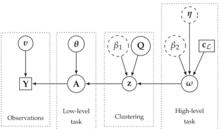
Fig. 1. Directed acyclic graph of the proposed hierarchical Bayesian model. (User- defined parameters appear in dotted circles and external data in squares). and illustrative instance of the proposed framework is presented in

Section4where hyperspectral images are analyzed under the dual scope of unmixing and classification. Finally, Section 5concludes the paper and opens some research perspectives to this work. 2. Bayesianmodel

In order to propose a unifying framework offering multi-level image analysis, a hierarchical Bayesian model is derived to relate the observations and the task-related parameters of interest. This model is mainly composed of three main levels. The first level, presented in Section2.1, takes care of a low-level modeling achieving latent structure analysis. The second stage then assumes that data samples (e.g., resulting from measurements) can be divided into several statistically homogeneous clusters through their respective latent structures. To identify the cluster memberships, these samples are assigned discrete labels which are a priori described by a non-homogeneous Markov random field (MRF). This MRF com- bines two terms: the first one is related to the potential of a Potts-MRF to promote spatial regularity between neighboring pixels; the second term exploits labels from the higher level to promote coherence between cluster and classification labels. This clustering process is detailed in Section 2.2. Finally, the last stage of the model, explained in Section 2.3, allows high-level labels to be estimated, taking advantage of the availability of external knowledge as ground-truthed or expert-driven data, akin to a conventional supervised classification task. The whole model and its dependences are summarized by the directed acyclic graph in Fig.1.

2.1. Low-levelinterpretation

The low-level task aims at inferring PR-dimensional latent vari-

able vectors ap (

∀

p∈ P ,

{

1 , . . . , P

}

) appropriate for representing P respective d-dimensional observation vectors yp in a subspace

of lower dimension than the original observation space, i.e., R≤d. The task may also include the estimation of the function or additional parameters of the function relating the unobserved and observed variables. By denoting Y= [ y1, . . . , yP] and A= [ a1, . . . , aP]

the d×P- and R×P- matrices gathering respectively the obser-

vation and latent variable vectors, this relation can be expressed through the general statistical formulation

Y

|

A,

υ

∼

9 (

Y;flat

(

A

)

,

υ

)

, (1)

where

9 (

·,

υ

)

stands for a statistical model, e.g., resulting from physical or approximation considerations, flat( ·) is a deterministic function used to define the latent structure and

υ

are possible additional nuisance parameters. In most applicative contexts aimed by this work, the model

9

( ·) and function flat( ·) are separable

(4)

with respect to the measurements assumed to be conditionally independent, leading to the factorization

Y

|

A,

υ

∼

P Y p=1

9 (

yp;flat

(

ap

)

,

υ

)

. (2)

It is worth noting that this statistical model will explicitly lead to the derivation of the particular form of the likelihood function in- volved in the Bayesian model.

The choice of the latent structure related to the function flat( ·) is application-dependent and can be directly chosen by the end- user. A conventional choice consists in considering a linear ex- pansion of the observed data yp over an orthogonal basis span-

ning a space whose dimension is lower than the original one. This orthogonal space can be a priori fixed or even learnt from the dataset itself, e.g., leveraging on popular nonparametric methods such as principal component analysis (PCA) [19]. In such case, the model (1) should be interpreted as a probabilistic counterpart of PCA [20] and the latent variables ap would correspond to

factor loadings. Similar linear latent factors and low-rank models have been widely advocated to address source separation problems, such as nonnegative matrix factorization [21]. As a typical illustration, by assuming an additive white and centered Gaus- sian statistical model

9

( ·) and a linear latent function f_lat( ·), the generic model (2)can be particularly instanced as

Y

|

A,s2∼ P Y p=1 N

¡

yp;Map,s2Id

¢

₍₃₎

where Id is the d×d identity matrix, M is a matrix spanning

the signal subspace and s2 is the variance of the Gaussian error, considered as a nuisance parameter. Besides this popular class of Gaussian models, this formulation allows other noise statistics to be handled within a linear factor modeling, as required when the approximation should be envisaged beyond a conventional Eu- clidean discrepancy measure [22], provided that

E[Y

|

A]=flat

(

A

)

.

From a different perspective, the generic formulation of the statistical latent structure (2)can also result from a thorough analysis of more complex physical processes underlying observed measurements, resulting in specific yet richer physics-based latent models

[11,23]. For sake of generality, this latent structure will not be specified in the rest of this manuscript, except in Section 4where the linear Gaussian model (3) will be more deeply investigated as an illustration in a particular applicative context.

2.2. Clustering

To regularize the latent structure analysis, the model is com- plemented by a clustering step as a higher level of the Bayesian hierarchy. Besides, another objective of this clustering stage is also to act as a bridge between the low- and high-level data inter- pretations, namely latent structure analysis and classification. The clustering is performed under the assumption that the latent variables are statistically homogeneous and allocated in several clusters, i.e., identities belonging to a same cluster are supposed to be distributed according to the same distribution. To identify the membership, each observation is assigned a cluster label zp∈ K ,

{

1 , . . . , K

}

where K is the number of clusters. Formally, the unknown latent vector is thus described by the following prior

ap

|

zp=k,

θk

∼

8(

ap;

θk

)

, (4)

where

8

is a given statistical model depending on the addressed

problem and governed by the parameter vector

θ

k characterizing

each cluster. As an example, considering this prior distribution as Gaussian, i.e.,

8(

ap;

θ

k

)

= N

(

ap;

ψ

k,

6

k

)

with

θ

k=

©ψ

k,

6

k

ª

,

would lead to a conventional Gaussian mixture model (GMM) for the latent structure, as in [24](see Section4).

One particularity of the proposed model lies in the prior on the cluster labels z = [ z1, . . . , zP] . A non-homogeneous Markov Random

Field (MRF) is used as a prior model to promote two distinct be- haviors through the use of two potentials. The first one is a local and non-homogeneous potential parameterized by a K-by- J matrix

Q. It promotes consistent relationships between the cluster labels z and some classification labels

ω

= [

ω

1, . . . ,

ω

P] where

ω

p∈ J ,

{

1 , . . . , J

}

and J is the number of classes. These classification labels

associated with high-level interpretation will be more precisely investigated in the third stage of the hierarchy in Section2.3. Pursu- ing the objective of analyzing images, the second potential is associated with a Potts-MRF [25] of granularity parameter

β

1 to promote a piecewise consistent spatial regularity of the cluster labels. The prior probability of z is thus defined as

P[_z

_|

_ω

_,_Q]₌ 1 C

(

ω

,Q

)

exp

Ã

X p∈P V1

(

zp,

ω

p,qzp,ωp

)

+X p∈P X p′_∈V₍_p₎ V2

(

zp,zp′

)

!

(5)

where V

(

p) stands for the neighborhood of p, qk,jis the kth ele-

ment of the jth column of Q. The two terms V1( ·) and V2( ·) are the classification-informed and Potts–Markov potentials, respectively, defined by

V1

(

k,j,qk, j

)

=log

(

qk, j

)

V2

(

k,k′

)

=

β

1

δ

(

k,k′

)

where

δ

( ·, ·) is the Kronecker function. Finally, C(

ω

,Q) stands for the normalizing constant (i.e., partition function) depending of

ω

and Q and computed over all the possible z fields [15]

C

(

ω

,Q

)

= X z∈KP exp

Ã

X p∈P V1

(

zp,

ω

p,qzp,ωp

)

+ X p∈P X p′_∈V₍_p₎ V2

(

zp,zp′

)

!

= X z∈KP Y p∈P qzp ,ωp exp

Ã

β

1 X p′∈V(p)

δ

(

zp,zp′

)

!

. (6)

The equivalence between Gibbs random fields and MRF stated by the Hammersley–Clifford theorem [15]provides the prior probability of a particular cluster label conditionally upon its neigh- bors P[zp=k

|

zV(p),

ω

p= j,qk,ωp]∝ exp

Ã

V1

(

k,j,qk, j

)

+ X p′_∈V₍_p₎ V2

(

k,zp′

)

!

(7)

where the symbol ∝ stands for “proportional to”.

The elements qk,jof the matrix Q introduced in the latter MRF

account for the connection between cluster k and class j, reveal-

ing a hidden interaction between clustering and classification. A high value of qk,j tends to promote the association to the clus-

ter k when the sample belongs to the class j. This interaction en-

coded through these matrix coefficients is unknown and thus motivates the estimation of the matrix Q. To reach an interpretation of the matrix coefficients in terms of probabilities of inter- dependency, a Dirichlet distribution is elected as prior for each column qj= [ q1,j, . . . , qK, j] T of Q= [ q1, . . . , qJ] which are assumed to

be independent, i.e.,

qj∼Dir

(

qj;

ζ

1,...,

ζ

K

)

. (8)

The nonnegativity and sum-to-one constraints imposed to the coefficients defining each column of Q allows them to be interpreted

(5)

as probability vectors. The choice of such a prior is furthermore motivated by the properties of the resulting conditional posterior distribution of qj, as demonstrated later in Section3. In the present

work, the hyperparameters

ζ

1, . . . ,

ζ

K are all chosen equal to 1, re-

sulting in a uniform prior over the corresponding simplex defined by the probability constraints. Obviously, when additional prior knowledge on the interaction between clustering and classification is available, these hyperparameters can be adjusted accordingly.

2.3. High-levelinterpretation

The last stage of the hierarchical model defines a classification rule. At this stage, a unique discrete class label should be at- tributed to each sample. This task can be seen as high-level in the sense that the definition of the classes can be motivated by their semantic meaning. Classes can be specified by the end-user and thus a class may gather samples with significantly dissimilar observation vectors and even dissimilar latent features. The clustering stage introduced earlier also allows a mixture model to be derived for this classification task. Indeed, a class tends to be the union of several clusters identified at the clustering stage, providing a hierarchical description of the dataset.

In this paper, the conventional and well-admitted setup of a supervised classification is considered. This setup means that a partial ground-truthed dataset cL is available for a (e.g., small) subset of samples. In what follows, L ⊂ P denotes the subset of observation indexes for which this ground-truth is available. This ground-truth provides the expected classification labels for observations indexed by L . Conversely, the index set of unlabeled samples for which this ground-truth is not available is noted U ⊂ P, with P = U + L and U ∩ L = ∅ . Moreover, the proposed model assumes that this ground-truth may be corrupted by class labeling errors. As a consequence, to provide a classification robust to these possible errors, all the classification labels of the dataset will be estimated, even those associated with the observations indexed by L . At the end of the classification process, the labels estimated for observations indexed by L will not be necessarily equal to the labels cLprovided by the expert or an other external knowledge.

Similarly to the prior model advocated for z (see Section 2.2), the prior model for the classification labels

ω

is a non- homogeneous MRF composed of two potentials. Again, a Potts-MRF potential with a granularity parameter

β

2is used to promote spatial coherence of the classification labels. The other potential is non-homogeneous and exploits the supervised information available under the form of the ground-truth map cL. In particular, it attends to ensure consistency between the estimated and ground- truthed labels for the samples indexed by L . Moreover, for the classification labels associated with the indexes in U (i.e., for which no ground-truth is available), the prior probability to belong to a given class is set as the proportion of this class observed in cL. This setting assumes that the expert map is representative of the whole scene to be analyzed in term of label proportions. If this assumption is not verified, the proposed modeling can be easily adjusted accordingly. Mathematically, this formal description can be summarized by the following conditional prior probability for a given classification label

ω

p P[

_ω

_p₌ _j

_|

_ω

_V₍_p₎_,_c_p_,

_ηp

]_∝ exp

Ã

W1

(

j,cp,

ηp

)

+ X p′_∈V₍_p₎ W2

(

j,

ω

p′

)

!

. (9)

As explained above, the potential W₂( ·, ·) ensures the spatial coherence of the classification labels, i.e.,

W2

(

j,j′

)

=

β

2

δ

(

j,j′

)

.

More importantly, the potential W1( j,cp,

η

p) defined by

W1

(

j,cp,

ηp

)

=







½

_log

(

η

p

)

, when j=cp log

(

1−ηp J−1

)

, otherwise , when p∈L log

(

π

j

)

, when p∈U

encodes the coherence between estimated and ground-truthed labels when available (i.e., when p∈ L) or, conversely for non- ground-truthed labels (i.e., when p ∈ U), the prior probability of assigning a given label through the proportion

π

j of samples of

class j in cL. The hyperparameter

η

p∈ (0, 1) stands for the confi-

dence given in cp, i.e., the ground-truth label of pixel p. In the case

where the confidence is total, the parameter tends to 1 and it leads to

ω

p = cpin a deterministic manner. However, in a more realistic

applicative context, ground-truth is generally provided by human experts and may contain errors due for example to ambiguities or simple mistakes. It is possible with the proposed model to set for example a 90% level of confidence which allows to re-estimate the class label of the labeled set L and thus to correct the provided ground-truth. By this mean, the robustness of the classification to label errors is improved.

3. Gibbssampler

To infer the parameters of the hierarchical Bayesian model introduced in the previous section, an MCMC algorithm is derived to generate samples according to the joint posterior distribution of interest which can be computed according to the following hierarchical structure

p

(

A,

2

,z,Q,

ω

|

Y

)

∝p

(

Y

|

A

)

p

(

A

|

z,

θ

)

p

(

z

|

Q,

ω

)

p

(

ω

)

with

2

,

©θ

1, . . . ,

θ

K

ª

. Note that, for conciseness, the nuisance parameters

υ

have been implicitly marginalized out in the hierarchical structure. If this marginalization is not straightforward, these nuisance parameters can be also explicitly included within the model to be jointly estimated.

The Bayesian estimators of the parameters of interest can then be approximated using these samples. The minimum mean square error (MMSE) estimators of the parameters A,

2

and Q can be approximated through empirical averages

ˆ xMMSE=E[x

|

Y]≈ 1 NMC NMC X t=1 x(t) ₍₁₀₎

where ·(t)_{denotes the}_t_{th samples and}_N

MCis the number of iterations after the burn-in period. Conversely, the maximum a posteri- ori estimators of the cluster and class labels, z and

ω

, respectively, can be approximated as

ˆ

xMAP=argmax

x p

(

x

|

Y

)

≈argmax_x(t)

p

(

x(t)

_|

_Y

₎

₍₁₁₎

which basically amounts at retaining the most frequently generated label for these specific discrete parameters [26].

To carry out such a sampling strategy, the conditional posterior distributions of the various parameters need to be derived. More importantly, the ability of drawing according to these distributions is required. These posterior distributions are detailed in what follows.

3.1. Latentparameters

Given the likelihood function resulting from the statistical model (2)and the prior distribution in (4), the conditional posterior distribution of a latent vectors can be expressed as follows: p

(

ap

|

yp,

υ

,zp=k,

θk

)

∝p

(

yp

|

ap,

υ

)

p

(

ap

|

zp=k,

θk

)

(6)

3.2. Clusterlabels

The cluster label zp being a discrete random variable, it is pos-

sible to sample the variable by computing the conditional probability for all possible values of zpin K

P

₍

_z_p=k

|

θk

,

ω

p=j,qk, j

)

∝p

(

ap

|

zp=k,

θ

k

)

P

(

zp=k

|

zV(p),

ω

p=j,qk, j

)

∝

8(

ap;

θk

)

qk, jexp

Ã

β

1 X p′_∈V₍_p₎

δ

(

k,z′ p

)

!

. (13) 3.3. Interactionmatrix

The conditional distribution of each column qj ( j ∈ J ) of the

interaction parameter matrix Q can be written p

(

qj

|

z,Q\j,

ω

)

∝p

(

qj

)

P

(

z

|

Q,

ω

)

∝ QK k=1q nk, j k, j C

(

ω

,Q

)

1 SK

(

qj

)

. (14)

where Q\j denotes the matrix Q whose jth column has been re-

moved, n_{k, j}= #

{

p

|

zp= k,

ω

p = j

}

is the number of observations

whose cluster and class labels are respectively k and j, and 1 S_K

(

·

)

is the indicator function of the K-dimensional probability simplex

which ensures that qj∈ SKimplies

∀

k∈ K, qk,j≥0 and PKk=1qk, j=

1 .

Sampling according to this conditional distribution would re- quire to compute the partition function C(

ω

, Q), which is not straightforward. The partition function is indeed a sum over all possible configurations of the MRF z. One strategy would consist in precomputing this partition function on an appropriate grid, as in [27]. As alternatives, one could use to likelihood-free Metropo- lis Hastings algorithm [28], auxiliary variables [29] or pseudo- likelihood estimators [30]. However, all these strategies remain of high computational cost, which precludes their practical use for most applicative scenarii encountered in real-world image analysis.

Besides, when

β

1= 0 , this partition function reduces to

C(

ω

, Q

)

= 1 . In other words, the partition function is constant when the spatial regularization induced by V2( ·) is not taken into account. In such case, the conditional posterior distribution for qj

is the following Dirichlet distribution

qj

|

z,

ω

∼Dir

(

qj;n1,j+1,...,nK, j+1

)

, (15)

which is easy to sample from. Interestingly, the expected value of

qk,jis then E

£

qk, j

|

z,

ω

¤

= nk, j+1 PK i=1ni,k+K

which is a biased empirical estimator of P [ zp= k

|

ω

p= j] . This lat-

ter result motivates the use of a Dirichlet distribution as a prior for qj. Thus, it is worth noting that Q can be interpreted as a byprod-

uct of the proposed model which describes the intrinsic dataset structure. It allows the practitioner not only to get an overview of the distribution of the samples of a given class in the various clusters but also to possibly identify the origin of confusions between several classes. Again, this clustering step allows disparity in the semantic classes to be mitigated. Intraclass variability results in the emerging of several clusters which are subsequently agglomerated during the classification stage.

In practice, during the burn-in period of the proposed Gibbs sampler, to avoid highly intensive computations, the cluster labels are sampled according to (13)with

β

1> 0 while the columns

of the interaction matrix are sampled according to (15). In other words, during this burn-in period, a certain spatial regularization with

β

1> 0 is imposed to the cluster labels and the interaction matrix is sampled according to an approximation of its conditional posterior distribution. 1 _{After this burn-in}_period,_{the granularity}

parameter

β

1is set to 0, which results in removing the spatial regularization between the cluster labels. Thus, once convergence has been reached, the conditional posterior distribution (15)reduces to

(14)and the iteraction matrix is properly sampled according to its exact conditional posterior distribution.

3.4.Classificationlabels

Similarly to the cluster labels, the classification labels

ω

are sampled by evaluating their conditional probabilities computed for all the possible labels. However, two cases need to be considered while sampling the classification label

ω

p, depending on the avail-

ability of ground-truth label for the corresponding pth pixel. More precisely, when p∈ U , i.e., when the pth pixel is not accompanied

by a corresponding ground-truth, the conditional probabilities are written P[

_ω

_p=j

|

z,

ω

\p,qj,cp,

ηp

] ∝P[_z_p

_|

ω

p= j,qj,zν(p)]P[

ω

p= j

|

ω

V(p),cp,

η

p] ∝ qzp ,j

π

jexp

¡β

2 P p′∈ν(p)

δ

(

j,

ω

p′

)

¢

PK k′₌₁qk′_,_jexp

¡β

₁P_p′_∈_ν(_p₎

δ

(

k′,zp′

)

¢

, (16)

where

ω

\p denotes the classification label vector

ω

whose pth el-

ement has been removed. Conversely, when p∈ L , i.e., when the

pth pixel is assigned a ground-truth label cp, the conditional pos-

terior probability reads

P[

_ω

_p=j

|

z,

ω

\p,qj,cp,

ηp

] ∝P[_z_p

_|

ω

p= j,qj,zν(p)]P[

ω

p= j

|

ω

V(p),cp,

η

p] ∝











qzp,jηpexp

(

β2P p′∈ν(p)δ(j,ωp′)

)

PK k′=1qk′,jexp

(

β1 P p′∈ν(p)δ(k′,zp′)

)

when

ω

p=cp (1−ηp)qzp,jexp

(

β2P p′∈ν(p)δ(j,ωp′)

)

(C−1)PK k′=1qk′,jexp

(

β1Pp′∈ν(p)δ(k′,zp′)

)

otherwise (17)

Note that, as for the sampling of the columns qj ( j ∈ J) of

the interaction matrix Q, this conditional probability is consid- erably simplified when

β

1= 0 (i.e., when no spatial regularization is imposed on the cluster labels) since, in this case, PK

k′₌₁qk′_,_jexp

(

β

1Pp′_∈_ν(_p₎

δ

(k

′, z_p′

))

= 1 .

4. Applicationtohyperspectralimageanalysis

The proposed general framework introduced in the previous sections has been instanced for a specific application, namely the analysis of hyperspectral images. Hyperspectral imaging for Earth observation has been receiving increasing attention over the last decades, in particular in signal/image processing literatures [31– 33]. This keen interest of the scientific community can be easily explained by the richness of the information provided by such images. Indeed, generalizing the conventional red/green/blue color imaging, hyperspectral imaging collects spatial measurements acquired in a large number of spectral bands. Each pixel is associated with a vector of measurements, referred to as spectrum, which characterizes the macroscopic components present in this

1_{This strategy can also be interpreted as choosing C (}_ω_,_{Q ) × Dir( 1 ) instead of the}

(7)

pixel. Classification and spectral unmixing are two well-admitted techniques to analyze hyperspectral images. As mentioned earlier, and similarly to numerous applicative contexts, classifying hyperspectral images consists in assigning a discrete label to each pixel measurement in agreement with a predefined semantic description of the image. Conversely, spectral unmixing proposes to re- trieve some elementary components, called endmembers, and their

respective proportions, called abundance in each pixel, associated with the spatial distribution of the endmembers in over the scene

[12]. Per se, spectral unmixing can be cast as a blind source separation or a nonnegative matrix factorization (NMF) task [34]. The particularity of spectral unmixing, also known as spectral mixture analysis in the microscopy literature [35], lies in the specific constraints applied to spectral unmixing. As for any NMF problem, the endmembers signatures as well as the proportions are nonnegative. Moreover, specifically, to reach a close description of the pixel measurements, the abundance coefficients, interpreted as concentrations of the different materials, should sum to one for each spatial position.

Nevertheless, yet complementary, these two classes of methods have been considered jointly in a very limited number of works [36,37]. The proposed hierarchical Bayesian model offers a great opportunity to design a unified framework where these two methods can be conducted jointly. Spectral unmixing is perfectly suitable to be envisaged as the low-level task of the model described in Section 2. The abundance vector provides a biophysical description of a pixel which can be seen as a vector of latent variables of the corresponding pixel. The classification step is more related to a semantic description of the pixel. The low-level and clustering tasks of general framework described, respectively, in

Sections2.1and 2.2, are specified in what follows, while the classification task is directly implemented as in Section2.3.

4.1. Bayesianmodel

Low-level interpretation: According to the conventional linear mixing model (LMM), the pixel spectrum yp ( p∈ P) observed in d

spectral bands are approximated by linear mixtures of R elementary signatures mr( r = 1 , . . . , R), i.e.,

yp=

R X r=1

ar,pmr+ep (18)

where ap = [ a1,p, . . . , aR,p] T denotes the vector of mixing coeffi-

cients (or abundances) associated with the pth pixel and ep is

an additive error assumed to be white and Gaussian, i.e., ep

|

s2∼

N

(

0d, s2Id

)

. When considering the P pixels of the hyperspectral

image, the LMM can be rewritten with its matrix form

Y=MA+E (19)

where M= [ m1, . . . , mR] , A= [ a1, . . . , aP] and E= [ e1, . . . , eP] are

the matrices of the endmember signatures, abundance vectors and noise, respectively. In this work, the endmember spectra are assumed to be a priori known or previously recovered from the hyperspectral images by using an endmember extraction algorithm

[12]. Under this assumption, the LMM matrix formulation defined by (19) can be straightforwardly interpreted as a particular instance of the low-level interpretation (1) by choosing the latent function flat( ·) as a linear mapping flat

(

A

)

= MA and the statistical model

9

( ·, ·) as the Gaussian probability density function parametrized by the variance s2.

In this applicative example, since the error variance s2is a nui-

sance parameter and generally unknown, this hyperparameter is included within the Bayesian model and estimated jointly with the parameters of interest. More precisely, the variance s2is assigned a

conjugate inverse-gamma prior and a non-informative Jeffreys hy- perprior is chosen for the associate hyperparameter

δ

s2

|

δ

∼ IG

(

s2;1,

δ

)

,

δ

∝1

δ

1 R+

(

δ

)

. (20)

These choices lead to the following inverse-gamma conditional posterior distribution s2

|

Y,A∼ IG

Ã

s2;1+Pd 2, 1 2 P X p=1

k

yp−Map

k

2

!

(21)

which is easy to sample from, as an additional step within the Gibbs sampling scheme described in Section3.

Clustering: In the current problem, the latent modeling

8

( ·; ·) in (4)is chosen as Gaussian distributions elected for the latent vectors ap( p∈ P),

ap

|

zp=k,

ψ

k,

6

k∼ N

(

ap;

ψ

k,

6

k

)

(22)

where

ψ

kand

6

kare the mean vector and covariance matrix asso-

ciated with the kth cluster. This Gaussian assumption is equivalent

to consider each high-level class as a mixture of Gaussian distributions in the abundance space. The covariance matrices are chosen as

6

k= diag

(

σ

k,21, . . . ,

σ

k,R2

)

where

σ

k,21, . . . ,

σ

k,R2 are a set of R un-

known hyperparameters. The conditional posterior distribution of the abundance vectors ap can be finally expressed as follows:

p

(

ap

|

zp=k,yp,

ψ

k,

6

k

)

∝

|

3

k

|

− 1 2exp

³

−1 2

(

ap−

µ

k,p

)

t

3

−1k

(

ap−

µ

k,p

)

´

(23) where

µ

k,p=

3

k

(

_s12Mtyp+

6

−1_k

ψ

k

)

and

3

k=

(

_s12MtM+

6

−1k

)

−1. It

shows that the latent vector apassociated with a pixel belonging to

the kth cluster is distributed according to the multivariate Gaussian distribution N

(

ap;

µ

k,p,

3

k

)

.

Moreover the variances

σ

_k,r2 are included into the Bayesian model by choosing conjugate inverse-gamma prior distributions

σ

_k,r2 ∼ IG

(

σ

_k,r2;

ξ

,

γ

)

(24)

where parameters

ξ

and

γ

have been selected to obtain vague pri- ors (

ξ

= 1 ,

γ

= 0 . 1 ). It leads to the following conditional inverse- gamma posterior distribution

σ

_r,k2

|

A,z,

ψ

r,k∼ IG

Ã

σ

_k,r2 ;nk 2 +

ξ

,

γ

+ X p∈Ik

(

ar,p−

ψ

r,k

)

2 2

!

(25)

where nkis the number of samples in cluster k, and I k⊂ P is the

set of indexes of pixels belonging to the kth cluster (i.e., such that zp= k).

Finally, the prior distribution of the cluster mean

ψ

k ( k ∈ K)

is chosen as a Dirichlet distribution Dir( 1). Such a prior induces

soft non-negativity and sum-to-one constraints on ap. Indeed, these

two constraints are generally admitted to describe the abundance coefficients since they represent proportions/concentrations. In this work, this constraint is not directly imposed on the abundance vectors but rather on their mean vectors, since E[ ap

|

zp= k] =

ψ

k.

The resulting conditional posterior distribution of the mean vector

ψ

kis the following multivariate Gaussian distribution

ψ

k

|

A,z,

6

k∼ NS_R

Ã

ψ

k; 1 nk X p∈Ik ap, 1 nk

6

k

!

(26)

truncated on the probability simplex

S_R=

(

x=[x1,...,xR]T

|∀

r, xr≥0 and R X r=1 xr=1

)

. (27)

Sampling according to this truncated Gaussian distribution can be achieved following the strategies described in [38].

(8)

Algorithm1: Inference using Gibbs sampling. 1 Initialize all variables;

2forNMC+ Nburniterationsdo

3 foreachp∈ P do sample apfrom N

(

µ

k,p,

3

k

)

;

4 foreachp∈ P do sample zpfrom (13);

5 foreach j∈ J do sample qjfrom

Dir

(n

1,j+ 1 , . . . , nK, j+ 1

)

;

6 foreachp∈ P do sample

ω

pfrom (16) and (17);

7 fork = 1 toK do 8 sample

ψ

_kfrom N S_R

³

1 nk P p∈Ikap, 1 nk

6

k

´

; 9 foreachr ∈

{

1 , . . . , R

}

do sample

σ

_r,k2 from

IG

³

nk 2 +

ξ

,

γ

+Pp∈Ik (ar,p−ψr,k)2 2

´

; 10 end 11 sample s2 from IG

¡

1 + Pd₂, 1₂PP p=1

k

yp−Map

k

2

¢

; 12 sample

δ

from IG

(

1 , s2

)

; 13 ifiteration > Nburnthen

14 update MMSE and MAP estimators

15 end

16end

Full inference procedure is summarized in Algorithm 1. It should be noticed that MMSE and MAP estimators are updated online at each iteration after the burn-in period in order to save storage and thus possibly handle large dataset. Additionally, the number of iteration is chosen in order to get a reasonable processing time.

4.2. Experiments 4.2.1. Syntheticdataset

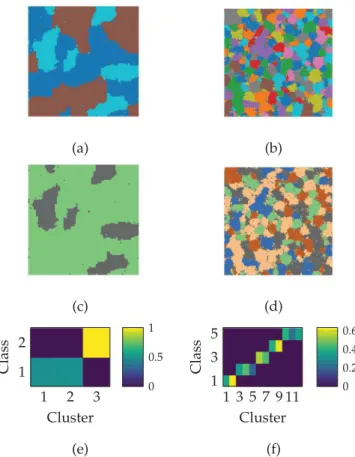
Synthetic data have been used to assess the performance of the proposed analysis model and algorithm. Two distinct images, referred to as Image 1 and Image 2 and represented in Fig.2, have been considered. The first one is a 100 ×100 pixel image composed of R = 3 endmembers, K = 3 clusters and J = 2 classes. The second hyperspectral image is a 200 ×200 pixel image which consists of R = 9 endmembers, K = 12 clusters and J = 5 classes. They have been synthetically generated according to the following hierarchical procedure. First, cluster maps have been generated from Potts–Markov MRFs to obtain (b) and (d) from Fig. 2. Then, the corresponding classification maps have then been chosen by artificially merging a few of these clusters to define each class and get (a) and (c) from Fig.2. For each pixel, an abundance vector ap has been randomly drawn from a Dirichlet distribution

parametrized by a specific mean for each cluster. Finally the pixel measurements Y have been generated using the linear mixture model with real endmembers signatures of d = 413 spectral bands extracted from a spectral library. These linearly mixed pixels have been corrupted by a Gaussian noise resulting in a signal-to-noise ratio of SNR = 30 dB. The real interaction matrix Q presented in

Fig. 2(e) and (f) summarized the data structure by providing the probability to be in a given cluster when belonging to a given class.

Fig. 3represents the abundance vectors of each pixel in the probabilistic simplex for Image 1. The three clusters are clearly identifiable and the class represented in blue is also clearly divided into two clusters.

To evaluate the interest of including the classification step into the model, results provided by the proposed method have been compared to the counterpart model proposed in [24] (referred to as Eches model). The Eches model is a similar model which lacks the classification stage and thus does not exploit this high-level

Fig. 2. Synthetic data. Classification maps of Image 1 (a) and Image 2 (b), corre- sponding clustering maps of Image 1 (c) and Image 2 (d), corresponding interaction matrix Q of Image 1 (e) and Image 2 (f).

Fig. 3. Image 1. Left: colored composition of abundance map. Right: pixels in the probabilistic simplex (red triangle) with Class 1 (blue) and Class 2 (green). (For interpretation of the references to colour in this figure legend, the reader is referred to the web version of this article).

information. Fig.4presents the directed acyclic graph summariz- ing the model and its dependences in this particular hyperspectral framework and outlining the difference with Eches model. The pixels and associated classification labels located in the upper quar- ters of the Images 1 and 2 have been used as the training set L . The confidence in this classification ground-truth has been set to a value of

η

p = 0 . 95 for all the pixels ( p∈ L ). Additionally, the

values of Potts-MRF granularity parameters have been selected as

β

1=

β

2= 0 . 8 . In the case of the Eches model, the images have been subsequently classified using the estimated abundance vectors and clustering maps, and following the strategy proposed in

[13]. The performance of the spectral unmixing task has been evaluated using the root global mean square error (RGMSE) associated with the abundance estimation

RGMSE

(

A

)

=

r

1 PR

°

Aˆ−A

°

2 F (28)

(9)

Table 1

Unmixing and classification results for various datasets.

RGMSE(A) Kappa Time (s)

Image 1 Proposed model 3.23e-03 (1.6e-05) 0.932 (0.018) 171 (5.4) Eches model 3.24e-03 (1.4e-05) 0.909 (0.012) 146 (0.7) Image 2 Proposed model 1.62e-02 (1.62e-04) 0.961 (0.04) 950 (11)

Eches model 1.61e-02 (2.71e-05) 0.995 (0.0 0 04) 676 (2.1) MUESLI image Proposed model N \ A 0.837 (5e-3) 7175 (102)

Random Forest N \ A 0.879 (5e-4) 34 (1.3)

Gaussian model N \ A 0.818 (8.7e-5) 4 (0.01)

Fig. 4. Directed acyclic graph of the proposed model in the described hyperspectral framework. Part in blue is the extension made to the Eches model. (For interpretation of the references to colour in this figure legend, the reader is referred to the web version of this article).

where _Aˆ and A denote, respectively, the estimated and actual matrices of abundance vectors. Moreover, the accuracy of the estimated classification maps has been measured with the conventional Cohen’s kappa. Results reported in Table1show that the obtained RGMSE are not significantly different between the two models. Moreover, the comparison between processing times shows a small computational overload required by the proposed model. It should be noticed that this experiment has been conducted with a fixed number of iterations of the proposed MCMC algorithm (300 iterations including 50 burn-in iterations).

A second scenario is considered where the training set includes label errors. The corrupted training set is generated by tuning a varying probability

α

to assign an incorrect label, all the other possible labels being equiprobable. The probability

α

varies from 0 to 0.4 with a 0.05 step. In this context, the confidence in the classification ground-truth map is set equal to

η

p= 1 −

α

(

∀

p∈ L ). The

results, averaged over 20 trials for each setting, are compared to the results obtained using a mixture discriminant analysis (MDA)

[39] conducted either directly on the pixel spectra, either on the abundance vectors estimated with the proposed model. The resulting classification performances for Image 1 are depicted in Fig.5

as function of

α

. These results show that the proposed model per- forms very well even when the training set is highly corrupted (i.e.,

α

close to 0.4).

Moreover, as already explained, another advantage of the proposed model is the interesting by-products provided by the method. As an illustration, Fig. 6presents the interactions matrices Q estimated for each image. From this figure, it is clearly possible to identify the structure of the various classes and their hierarchical relationship with the underlying clusters. For instance, for Image 2, it can be noticed that Class 1 is essentially composed of two clusters which is confirmed by the true interaction matrix presented in Fig.2(e).

A last scenario has been considered in order to show the interest of the proposed method in term of spectral unmixing. A more

Fig. 5. Classification accuracy measured with Cohen’s kappa as a function of label corruption α: proposed model (red), MDA with abundance vectors (blue) and MDA with measured reflectance (blue). Shaded areas denote the intervals corresponding to the standard deviation computed over 20 trials. (For interpretation of the references to color in this figure legend, the reader is referred to the web version of this article).

Fig. 6. Estimated interaction matrix Q for Image 1 (top) and Image 2 (bottom).

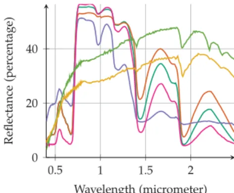
Fig. 7. Spectra used to generate the semi-synthetic image. 4 spectra are vegetation spectra and 2 are soil spectra.

complex synthetic image has been generated to assess this point. A 100 ×250-pixel real hyperspectral image has been unmixed using the fully constrained optimization method described in [40]. The obtained realistic abundance maps have been used to generate a new image with new real endmembers signatures of d = 252 spectral bands extracted from a spectral library. The selected endmembers presented in Fig.7has been chosen in order to be highly correlated (4 vegetation spectra and 2 soils spectra). Moreover the endmembers matrix M has been augmented by 9 endmembers not

(10)

Fig. 8. Semi-synthetic image. Panchromatic view of the hyperspectral image (a), ground-truth (b).

Fig. 9. Evolution of RGMSE of the sampled ˆ A(t) matrix in function of the time for the proposed model (red) and Eches model (blue). Results are averaged in time and score over 10 trials. (For interpretation of the references to color in this figure legend, the reader is referred to the web version of this article).

Fig. 10. Semi-synthetic image. Example of error map ( ° °ˆ ap − a p °

°₂_{) for proposed} model (a), example of error map for Eches model (b).

present in the image. The obtained data is indeed both realistic and challenging in term of unmixing. A panchromatic view of the resulting image, made by summing all spectral bands, is presented in Fig.8along with the ground-truth retrieved from the one provided with the original image with J = 4 classes. A Gaussian noise is finally added to this semi-synthetic image to get a signal-to- noise ratio of SNR = 10 dB.

Fig.9shows the evolution of RGMSE computed at each iteration for 250 iterations using the sampled Aˆ (t) _{matrix and the known}

A abundance matrix. For this experiment, the whole classification ground-truth was provided to the proposed algorithm as expert data cL and parameters have been set to

β

1 = 0 . 3 and

β

2 = 1 . 2 for the proposed model and

β

1 = 1 . 2 for Eches model. The evolution of the RGMSE is presented in function of the time since iteration are longer with the proposed model than with Eches model. Contrary to one would expect, the proposed model appears to be much faster to converge in number of iterations resulting in a convergence in the same time than Eches model. The increase of com- plexity and processing time is compensated by the fact that the classification information help significantly the convergence. More- over as shown in Fig. 10, the error made by the proposed model tends to be more spatially coherent than the error made by Eches model which are sometimes scattered in small area. This limita- tion of Eches model is induced by the tendency to over-segment the image in more clusters than necessary.

4.2.2. Realhyperspectralimage

Finally, the proposed strategy has been implemented to analyze a real 600 ×600-pixel hyperspectral image acquired within the framework of the multiscalemapping ofecosystem services by

Fig. 11. Real MUESLI image. Colored composition of the hyperspectral image (a), expert ground-truth (b), estimated clustering (c), training data (d), estimated classification with proposed model (e) and estimated classification with random forest (f).

very high spatial resolution hyperspectral and LiDAR remote sens-ingimagery (MUESLI) project 2 _{This image is composed of}_d_{= 438}

spectral bands and R = 7 endmembers have been extracted using the widely-used vertex component analysis (VCA) algorithm [41]to obtain matrix M. The associated expert ground-truth classification is made of 6 classes (straw cereals, summer crops, wooded area, buildings, bare soil, pasture). In this experiment, the upper half of the expert ground-truth has been provided as training data for the proposed method. The confidence

η

p has been set to 95% for all

training pixels to account for the imprecision of the expert ground- truth. The MRF granularity parameters of the proposed parameters have been set to

β

1 = 0 . 3 and

β

2 = 1 since these values provide the most meaningful interpretation of the image. Fig.11presents a colored composition of the hyperspectral image (a), the expert ground-truth (b) and the obtained results in terms of clustering (c) and classification (d). Quantitative results in term of classification accuracy have been computed and are summarized in Table1. Note that no performance measure of the unmixing step is provided since no abundance ground-truth is available for this real dataset.

For comparison purposed, classification has been conducted with two conventional classifier namely random forest (RF) and a Bayesian Gaussian model (GM) using scikit-learn library. Pa- rameters of the two classifiers have been optimized using cross- validation on the training set. Additionally, a principal component analysis has been used in order to reduce dimension before feating the Gaussian model. The proposed method appears to be compet- itive with these classifiers in term of classification at the cost of an increase of processing time. It is nevertheless important to note that the proposed method conducts additionally a spectral unmixing and estimates by-products of high interest for the user, for example matrix Q.

(11)

Fig. 12. Real MUESLI image. Classification accuracy measured with Cohen’s kappa as a function of label corruption α: proposed model (red), random forest (blue), PCA +Gaussian model (green). Shaded areas denote the intervals corresponding to the standard deviation computed over 10 trials. (For interpretation of the references to color in this figure legend, the reader is referred to the web version of this article.) Additionally, the robustness with respect to expert mislabeling of the ground-truth training dataset has been evaluated and compared to the performance obtained by a state-of-the-art random forest (RF) classifier. Errors in the expert ground-truth have been randomly generated with the same process as the one used for the previous experiment with synthetic data (see Section4.2.1). Confi- dence in the ground-truth has been set equal to

η

p= 1 −

α

for all

the pixels ( p∈ L ) where

α

is the corruption rate, with a maximum of 95% of confidence. Parameters of the RF classifier have been optimized using cross-validation on the training set. Classification accuracy measured through Cohen’s kappa is presented in Fig.12as a function of the corruption rate

α

of the training set. From these results, the proposed method seems to perform favorably when compared to the RF classifier. It is worth noting that RF is one of the prominent method to classify remote sensing data and that the robustness to noise in labeled data is a well-documented property of this classification technique [14].

5. Conclusionandperspectives

This paper proposed a Bayesian model to perform jointly low- level modeling and robust classification. This hierarchical model capitalized on two Markov random fields to promote coherence between the various levels defining the model, namely, (i) between the clustering conducted on the latent variables of the low-level modeling and the estimated class labels, and (ii) between the estimated class labels and the expert partial label map provided for supervised classification. The proposed model was specifically de- signed to result into a classification step robust to labeling errors that could be present in the expert ground-truth. Simulta- neously, it offered the opportunity to correct mislabeling errors. This model was particularly instanced on a particular application which aims at conducting hyperspectral image unmixing and classification jointly. Numerical experiments were conducted first on synthetic data and then on real data. These results demonstrate the relevance and accuracy of the proposed method. The richness of the resulting image interpretation was also underlined by the results. Future works include the generalization of the proposed model to handle fully unsupervised low-level analysis tasks. In- stantiations of the proposed model in other applicative contexts will be also considered.

References

[1]C.S. Won , R.M. Gray , Stochastic Image Processing, Information Technology: Transmission, Processing, and Storage, Springer Science & Business Media, New York, 2013 .

[2] J. Kersten , Simultaneous feature selection and Gaussian mixture model estimation for supervised classification problems, Pattern Recognit. 47 (8) (2014) 2582–2595 .

[3] N. Dobigeon , J.-Y. Tourneret , C.-I. Chang , Semi-supervised linear spectral unmixing using a hierarchical Bayesian model for hyperspectral imagery, IEEE Trans. Signal Process. 56 (7) (2008) 2684–2695 .

[4] M. Fauvel , J. Chanussot , J.A. Benediktsson , A spatial-spectral kernel-based approach for the classification of remote-sensing images, Pattern Recognit. 45 (1) (2012) 381–392 .

[5] T. Hastie , R. Tibshirani , J. Friedman , The Elements of Statistical Learning, Springer Series in Statistics, Springer New York, New York, NY, 2009 .

[6] G.M. Foody , A. Mathur , The use of small training sets containing mixed pixels for accurate hard image classification: training on mixed spectral responses for classification by a SVM, Remote Sens. Environ. 103 (2006) 179–189 .

[7] L.O. Jimenez , D.A. Landgrebe , Supervised classification in high-dimensional space: geometrical, statistical, and asymptotical properties of multivariate data, IEEE Trans. Syst. Man Cybern. - Part C 28 (1) (1998) 39–54 .

[8] R. Sheikhpour , M.A. Sarram , S. Gharaghani , M.A.Z. Chahooki , A survey on semi– supervised feature selection methods, Pattern Recognit. 64 (2017) 141–158 .

[9] A. Lagrange , M. Fauvel , M. Grizonnet , Large-scale feature selection with Gaus- sian mixture models for the classification of high dimensional remote sensing images, IEEE Trans. Comput. Imaging 3 (2) (2017) 230–242 .

[10] A. Ozerov , C. Févotte , R. Blouet , J.-L. Durrieu , Multichannel nonnegative tensor factorization with structured constraints for user-guided audio source separation, in: Proceedings of the IEEE International Conference on Acoustics, Speech and Signal Processing (ICASSP), 2011, pp. 257–260 .

[11]M. Pereyra , N. Dobigeon , H. Batatia , J.Y. Tourneret , Segmentation of skin le- sions in 2-D and 3-D ultrasound images using a spatially coherent generalized Rayleigh mixture model, IEEE Trans. Med. Imaging 31 (2012) 1509–1520 .

[12] J.M. Bioucas-Dias , A. Plaza , N. Dobigeon , M. Parente , Q. Du , P. Gader , J. Chanus- sot , Hyperspectral unmixing overview: geometrical, statistical, and sparse re- gression-based approaches, IEEE J. Sel. Top. Appl. Earth Obs. Remote Sens. 5 (2012) 354–379 .

[13] C. Bouveyron , S. Girard , Robust supervised classification with mixture models: learning from data with uncertain labels, Pattern Recognit. 42 (2009) 2649–2658 .

[14] C. Pelletier , S. Valero , J. Inglada , N. Champion , C. Marais Sicre , G. Dedieu , Ef- fect of training class label noise on classification performances for land cover mapping with satellite image time series, Remote Sens. 9 (2017) 173 .

[15] S.Z. Li , Markov Random Field Modeling in Image Analysis, Springer Science & Business Media, 2009 .

[16] Y. Zhang , M. Brady , S. Smith , Segmentation of brain MR images through a hidden Markov random field model and the expectation-maximization algorithm, IEEE Trans. Med. Imaging 20 (2001) 45–57 .

[17] Y. Tarabalka , M. Fauvel , J. Chanussot , J.A. Benediktsson , SVM- and MRF-based method for accurate classification of hyperspectral images, IEEE Geosci. Re- mote Sens. Lett. 7 (2010) 736–740 .

[18] F. Chen , K. Wang , T. Van de Voorde , T.F. Tang , Mapping urban land cover from high spatial resolution hyperspectral data: an approach based on simultaneously unmixing similar pixels with jointly sparse spectral mixture analysis, Re- mote Sens. Environ. 196 (2017) 324–342 .

[19] M. Fauvel , J. Chanussot , J.A. Benediktsson , Kernel principal component analysis for feature reduction in hyperspectrale images analysis, in: Proceedings of the Nordic Signal Processing Symposium (NORSIG), 2006, pp. 238–241 .

[20]M.E. Tipping , C.M. Bishop , Probabilistic principal component analysis, J. R. Stat. Soc. Ser. B 61 (3) (1999) 611–622 .

[21]C. Févotte , N. Bertin , J.-L. Durrieu , Nonnegative matrix factorization with the Itakura–Saito divergence. With application to music analysis, Neural Comput. 21 (3) (2009) 793–830 .

[22] C. Févotte , J. Idier , Algorithms for nonnegative matrix factorization with the beta-divergence, Neural Comput. 23 (9) (2011) 2421–2456 .

[23] M. Albughdadi , L. Chaari , F. Forbes , J.Y. Tourneret , P. Ciuciu , Model selection for hemodynamic brain parcellation in FMRI, in: Proceedings of the European Signal Processing Conference (EUSIPCO), 2014, pp. 31–35 .

[24]O. Eches , N. Dobigeon , J.-Y. Tourneret , Enhancing hyperspectral image unmixing with spatial correlations, IEEE Trans. Geosci. Remote Sens. 49 (2011) 4239–4247 .

[25] F.-Y. Wu , The Potts model, Rev. Mod. Phys. 54 (1982) 235 .

[26] G. Kail , J.-Y. Tourneret , F. Hlawatsch , N. Dobigeon , Blind deconvolution of sparse pulse sequences under a minimum distance constraint: a partially collapsed Gibbs sampler method, IEEE Trans. Signal Process. 60 (6) (2012) 2727–2743 .

[27]L. Risser , T. Vincent , J. Idier , F. Forbes , P. Ciuciu , Min-max extrapolation scheme for fast estimation of 3D Potts field partition functions. Application to the joint detection-estimation of brain activity in fMRI, J. Signal Process Syst. 60 (1) (2010) 1–14 .

[28] M. Pereyra , N. Dobigeon , H. Batatia , J.-Y. Tourneret , Estimating the granularity coefficient of a Potts–Markov random field within an MCMC algorithm, IEEE Trans. Image Process. 22 (6) (2013) 2385–2397 .

[29] J. Moller , A.N. Pettitt , R. Reeves , K.K. Berthelsen , An efficient Markov chain Monte Carlo method for distributions with intractable normalising constants, Biometrika 93 (2) (2006) 451–458 .

[30]J. Besag , Statistical analysis of non-lattice data, J. R. Stat. Soc. Ser. D 24 (3) (1975) 179–195 .

[31] G. Camps-Valls , D. Tuia , L. Bruzzone , J.A. Benediktsson , Advances in hyperspectral image classification: Earth monitoring with statistical learning methods, IEEE Signal Process. Mag. 31 (1) (2014) 45–54 .