Weighted estimate of extreme quantile: An application to the estimation of high flood return periods

Weighted estimate of extreme quantile : an application

to the estimation of high flood return periods

Alexandre Lekina

_{, Fateh Chebana}

_{, Taha B. M. J. Ouarda}

November 2, 2012

Abstract

Parametric models are commonly used in Frequency Analysis of extreme hydrological events. To estimate extreme quantiles associated to high return periods, these models are not always appropriate. Therefore, estimators based on Extreme value Theory (EVT) are proposed in the literature. The Weissman estimator is one of the popular EVT-based semi-parametric estimators of extreme quantiles. In the present paper we propose a new family of EVT-based semi-parametric estimators of extreme quantiles. To built this new family of estimators, the basic idea consists in assigning the weights to the k observations being used. Numerical experiments on simulated data are performed and a case study is presented. Re-sults show that the proposed estimators are smooth, stable, less sentitive, and less biased than Weissman estimator.

Keywords : flood, extreme quantile, bias reduction, heavy tailed distribution, order

statis-tics, Weissman estimator.

∗_{Corresponding author, Alexandre.Lekina@ete.inrs.ca.}

†_{Canada Research Chair to the Estimation of Hydro-meteorological Variables, INRS-ETE, 490 rue de la}

Couronne, Quebec, Canada G1K 9A9.

1

Introduction

1

Extreme events and natural disasters (e.g. earthquakes, floods, storms, droughts, nuclear

ac-2

cidents, stock market crashes) dominate the daily news by their unpredictable nature. Given

3

their considerable economic and social impacts, it is of high importance to develop the

ap-4

propriate models for the prediction of these events. Frequency analysis (FA) procedures are

5

commonly used for the analysis of extreme hydrological events. The main goal of the FA of

6

flood events is the assessment of the probability of exceedence of an event xT, i.e. P(X > xT).

7

Alternatively, given a return period T , it is also of interest to estimate the quantity xT such

8

that P(X > xT) = 1/T . The event xT corresponds to the quantile associated to a return

9

period T (e.g. Salvadori et al., 2007, chapter 1).

10

In hydrology, the floods xT of interest are typically such that T is larger than n, where n

11

denotes the sample size (for instance, the number of years of record at the gauging site). The

12

traditional estimation procedure of xT or T consists in choosing a parametric probability

13

model f (x; θ) that is fully indexed by a finite parameter set θ (e.g. shape, scale and location

14

parameters). Once the parameters θ of the model are estimated, the exceedance probability

15

1/T (resp. quantile xT) is evaluated directly through the Cumulative Distribution Function

16

(CDF) F (x; θ) of the fitted distribution (resp. via an estimator of the generalized inverse of

17

F (x; θ)) (e.g. Young-Il et al., 1993; Haddad and Rahman, 2011).

18

Despite all efforts, the topic of the choice of the best fitting parametric probability model

19

f (x; θ) and parameter estimation method for flood FA remains elusive (Bobée et al., 1993).

20

In some countries, standard distributions are recommended to fit hydrometeorological

vari-21

ables, e.g. the Generalized Extreme Value (GEV) distribution in the United Kingdom for flood

22

FA and in the United States for precipitation, the Log-Pearson type 3 distribution in the United

23

States and China for streamflows, the Lognormal distribution in China for low flows and

24

floods (e.g. Chen et al., 2004; Chebana et al., 2010). Nevertheless, in practice several

prob-25

lems remain to be solved.

26

The FA approach based on the selection of a parametric probability distribution has a

27

number of drawbacks especially for large T . First, this approach relies heavily on the initial

28

choice of the parametric family of probability distributions. If this choice of distribution is

in-29

appropriate then, especially for large values of T , significant errors in quantile estimates are

obtained. Second, the sample sizes of hydrological records are often too short for the

appro-31

priate selection of the best fitting distribution. Stedinger (2000) recommended a minimum

32

sample size (n = 50) for robust estimates of quantiles. However, this size is often not

suffi-33

cient to make the judicious choice of the appropriate distribution by using goodness-of-fit

34

tests (e.g. Adlouni et al., 2008). The latter are rather sensitive to the behavior of the tail of the

35

distribution. Third, the classical parametric estimation procedures are heavily weighted

to-36

wards fitting the main body (central region) of the assumed probability density. On the other

37

hand, they attribute a relatively low weight to the estimation of the distribution tail.

More-38

over, Young-Il et al. (1993) argued that this estimation procedure is an onerous mismatch in

39

objectives since such parametric fits are not robust to outliers in the tail of the sample

distri-40

bution. Also, as natural disasters may come from different causes, this can lead to mixtures

41

of distributions. The tail behavior of a mixture is often dictated by the tail behavior of the

42

distribution with the heaviest tail and by the relative proportion of events that correspond to

43

each component (e.g. Young-Il et al., 1993).

44

The above drawbacks indicate that the parametric approach can be relatively unreliable.

45

Since non-parametric approaches capture better any distributional features homogeneous

46

or heterogeneous exhibited by the data, Apipattanavis et al. (2010) proposed a non-parametric

47

FA estimator based on local polynomial regression. Notice that Adamowski et al. (1998) showed

48

the advantages of using non-parametric methods in flood FA for both annual maximum and

49

partial duration flood series. The local polynomial regression does not require a “priori”

as-50

sumption of the underlying CDF and the estimation is local and data driven. The local

as-51

pect of the estimation provides the ability to capture any arbitrary features that might be

52

present in the data. Kernel-based estimators have been studied respectively by (Lall et al.,

53

1993; Moon and Lall, 1994), and Quintela-del-Río and Francisco-Fernández (2011) for flood

54

FA and air quality modeling. In Regional flood frequency estimation, Epanechnikov kernel

55

has been used by Ouarda et al. (2001)

56

Moreover, several authors have investigated methods based on the extreme value theory

57

(EVT) (Fisher and Tippet, 1928; Gnedenko, 1943). These methods are based on the

prop-58

erties of the k upper order statistics of the sample and on extrapolation methods. Currently,

59

three main categories of methods can be identified : (i) extrapolation method based on (GEV)

(e.g. Prescott and Walden, 1980; Smith, 1985; Hosking et al., 1985; Guida and Longo, 1988);

61

(ii) extrapolation method based on the excesses method and Generalized Pareto

Distribu-62

tions (GPD) (e.g. Balkema and de Haan, 1974; Pickands, 1975; Hosking and Wallis, 1987; Lang et al.,

63

1999) with its variants so-called exponential tail and quadratic tail (Breiman et al., 1990); (iii)

64

the semi-parametric and non-parametric methods (e.g. Hill, 1975; Pickands, 1975; Weissman,

65

1978; Dekkers and de Haan, 1989; Beirlant et al., 2005). All three categories are based on the

66

statistical model given by the maximum domain of attraction (MDA) condition that governs

67

EVT. Some comparison studies (theory and simulation) between the different methods can

68

be found in Rosen and Weissman (1996); de Haan and Peng (1998); Tsourti and Panaretos (2001).

69

In the semi-parametric approach, one seeks to develop estimators of the right tail

quan-70

tiles according to the tail behavior of the distribution. Thus, one assumes a parametric form

71

only for the tail part and not for the entire probability density. The methods based on this

ap-72

proach are more flexible than parametric ones. The well-known Weissman (1978) estimator

73

is a semi-parametric estimator of extreme quantiles. However, most semi-parametric

estima-74

tors of quantiles xTshare a number of common problems. Most importantly, they are biased

75

and sensitive to the selection of the k upper order statistics of the sample (Gomes and Oliveira,

76

2001).

77

The main objective of the present paper is to show that the usual practice in

hydrologi-78

cal FA to estimate quantiles by inverting the CDF is not appropriate for extreme quantiles.

79

Therefore, we present a number of alternatives to estimate these quantiles including, for

in-80

stance, the Weissman (1978) estimator. In addition, we propose a new family of EVT-based

81

semi-parametric estimators of extreme quantiles that are smooth, stable, less sentitive to the

82

number of observations being used, and less biased than Weissman (1978) estimator.

83

The paper is organized as follows. In section 2, we present the statistical framework of the

84

study and the background of EVT. In section 3, we propose the estimators of quantiles from

85

heavy-tailed distributions. The numerical experiments on simulated data are presented and

86

discussed in section 4 and the case study is carried out in section 5. Conclusions and some

87

directions for future work are presented in section 6.

2

Statistical framework and background of EVT

89

2.1

General statistical framework

90

Let us denote by F the CDF of a random variable X and xpthe associated quantile of order

1 − p defined by :

P(X ≤ xp) = 1 − P(X > xp) = F (xp) = 1 − p, for p ∈ (0, 1). (1)

We consider a sample {Xi, i = 1, . . . , n} of independent and identically distributed random

variables with distribution function F . We denote by X1,n≤ . . . ≤ Xn,ntheir associated order

statistics. From the observations of these variables, the aim is to built an estimator of the quantile xpwhen p = 1/T is very small, i.e. close to zero since the return period T is large. In

this context, we talk about high return period. Given any p ∈ (0, 1), the quantile xpis defined

via the generalized inverse of the CDF, i.e. xp = F←(1 − p). Thus a natural estimator of xpis

given by :

ˆ x_p = ˆFn

←

(1 − p), (2)

where ˆFnis an estimator of the CDF F . In Extreme value analysis, in order to preserve (in the

asymptotic analysis) the fact that the number of observations np above the quantile xpshould

be much smaller than any positive constant, one assumes that p depends on n, i.e. p = pn,

and that pn → 0 as n increases (e.g. Dekkers and de Haan, 1989; de Haan and Ferreira, 2006).

The terms extreme quantile, large quantile or high quantile mean that pnconverges to zero,

see e.g. Gardes et al. (2010) and Embrechts et al. (1997, chapter 6). In particular, for n large enough, the non-exceedance probability P(Xn,n< xp), can be approximated as :

P (Xn,n< xp) & e−npnas pn → 0, (3)

which represents the probability that the quantity of interest xpfalls outside the range of the

91

sample. From a mathematical point of view, two cases can be considered from (3).

Depend-92

ing on the rate of convergence of pnto zero, the probability in (3) could be 0 or not :

93

First, if pn→ 0 and npn → ∞ as n → ∞, then P(Xn,n < xp) → 0. In this situation, pngoes

94

to zero slower than 1/n and xpis eventually almost surely smaller than the largest observation

Xn,n. Consequently, the estimation of the extreme quantile requires to interpolate inside the

96

sample. In this context, the natural and basic estimator of xpis given by (2). For instance, the

97

(npn)-th largest observation of the sample {Xi, i = 1, . . . , n}, i.e. Xn−#npn$+1,n, is an option 98

(refer to Rényi, 1953; Dekkers and de Haan, 1989), where the symbol (•) denotes the floor

99

function.

100

Second, if pn → 0 and npn → c *= ∞ as n → ∞, then P(Xn,n< xp) → e−c. In this context,

101

the estimation of extreme quantiles may need extrapolation beyond the observations since

102

xpcould be outside the sample, i.e. after the largest observation. According to the value of c,

103

two situations arise :

104

When c ∈ [1, ∞), it is possible to estimate xpby (2), or basically by the (c)-th largest

ob-105

servation of the sample, since the estimation is based on the largest observations located

106

near the border of the sample, but still within the data set. Nevertheless, recall that the (c)-th

107

largest observation of a sample is asymptotically not Gaussian (Embrechts et al., 1997,

corol-108

laire 4.2.4).

109

When c ∈ [0, 1), then pngoes to zero at the same speed or faster than 1/n and xpis

even-110

tually larger that the maximal observation Xn,nwith probability e−c≥ e−1. In this case, the

111

estimation of xpis more difficult since it requires an estimation outside the sample. For

in-112

stance, the quantile of order (1−pn) with pn < 1/n is extreme and is eventually larger than the

113

maximum observation of the sample. Therefore, it is not appropriate to estimate it simply by

114

inverting the CDF F . In predictions, the values of quantiles exceeding the length of the series

115

are generally extrapolation values that exceed the largest observation of the sample.

116

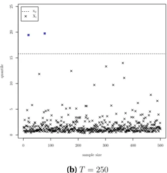
We illustrate in Figure 1 the difference between large quantiles within and outside the

117

sample. More precisely, Figures 1-(a) and 1-(b) describe the large quantile within the sample,

118

while Figure 1-(c) describes the large quantile outside the sample. To illustrate the difference

119

between the two quantiles, we generated a Fréchet distributed sample of size n = 500. In

120

hydrology, this distribution is applied to extreme events such as river discharges and annual

121

maximum 1-day rainfall (e.g. Coles, 2001).

122

In Figure 1-(a), p = 1/25 = 0.04 and the quantile x1/25is clearly smaller than the largest

123

observation of the sample. Since we have c = 20 observations above x1/25, then a

non-124

parametric estimator of quantile x1/25 obtained by interpolation is the 20-th largest

vation, i.e. X481,500. In Figure 1-(b), p = 1/250 = 0.004 and the estimation of the quantile

126

becomes difficult since it is based on the c = 2 observations above x1/250and located near

127

the border of the sample. In the case of Figure 1-(c) p = 1/600 & 0.0017 and the quantile

128

x1/600 is larger than the largest observation of the sample. To estimate x1/600one needs to

129

extrapolate beyond the largest observation of the sample.

130

When the number of observations above xp is finite, i.e. c *= ∞, one has to extend the

131

empirical distribution function beyond the sample. EVT studies the behavior of the k largest

132

observations of a sample and provides laws governing these values, and as such forms the

133

natural framework for estimating the event xpwhen c ∈ [0, 1), where the quantile of interest

134

is eventually larger than the maximal observation.

135

de Haan (1984) has established the first result in the case where c = 0. Dekkers and de Haan

136

(1989) have studied the case c = ∞ and c ∈ [0, 1). A summary of these results can be

137

found in (Embrechts et al., 1997, Theorem 6.4.14 and Theorem 6.4.15). Gardes et al. (2010),

138

Daouia et al. (2011) and Lekina (2010) provide an extension of situations c = ∞, c ≥ 1 and

139

c ∈ [0, 1) in the conditional case, that is to say in the situation where the variable of interest X

140

is recorded simultaneously with some covariate information. In the next section, we present

141

a brief summary of EVT.

142

2.2

EVT background

143

In the literature, several estimation methods of the extreme quantile xp where p & 0 have

been proposed, for instance in finance (Embrechts et al., 1997), in engineering structures (Ditlevsen, 1994) and in hydrology (Smith, 1987, 1986). These methods are based on the sta-tistical model given by the MDA condition that governs EVT (Fisher and Tippet, 1928; Gnedenko, 1943). The main result of EVT shows that under some regularity conditions on the CDF F of X, there exist a parameter γ ∈ R and two sequences (an)n≥1 > 0 and (bn)n≥1 ∈ R such that

for all x ∈ R, lim n→∞P ! Xn,n− bn an ≤ x " = Hγ(x), (4)

where Hγ(.) is a non-degenerate extreme value distribution defined by Hγ(x) =      exp_{'−(1 + γx)}−1/γ( if γ *= 0 exp [− exp(−x)] if γ = 0

and for all x such that 1 + γx > 0. (5)

The main result in (4) is true for most usual distributions F . If we make a parallel with the

144

Central Limit Theorem (CLT), the sequence anplays the role of n−1/2σ(X) where σ(X)

de-145

notes the standard deviation of X and the sequence bnplays the role of the mathematical

ex-146

pectation of X. The sequences anand bnare respectively interpreted as scale and location

pa-147

rameters. Note that these sequences are not unique. The reader is referred to Embrechts et al.

148

(1997) for some examples of anand nnin the fields of insurance and finance. A limited

num-149

ber of examples are presented in Table 1.

150

The parameter γ in (5) is called extreme value index and it has no equivalent in CLT. This

151

index is known to be the crucial indicator for the decay behaviour of the distribution tail.

152

It clearly governs the tail behavior, with larger values indicating heavier tails. If the cdf F

153

satisfies the Fisher and Tippet (1928) theorem conditions, then F belongs to MDA of Hγ(.).

154

According to the sign of γ, we distinguish the cases :

155

• Fréchet MDA (γ > 0) includes the distributions with polynomially decreasing

Pareto-156

type tails, e.g. Cauchy, Pareto and Burr. This family has a rather heavy right tail;

157

• Weibull MDA (γ < 0) includes the distributions with finite right endpoint, e.g. uniform

158

and beta;

159

• Gumbel MDA (γ = 0) includes distributions with exponentially decreasing tails, e.g.

nor-160

mal, exponential and Gamma. The distributions of this MDA are rather light tailed.

161

To check the assumption that F belongs to MDA of Hγ(.), several techniques are available.

For a review on exploratory data analysis methods for extremes the reader is refereed e.g. to Embrechts et al. (1997, section 6.2). In extreme value-analysis, the Pareto quantile plot (PQ-plot) is based on :

)* logn + 1 j , Xn−j+1 + , j = 1, . . . , n , , (6)

and is widely used to graphically check if data are distributed according to a MDA(Fréchet) or not. If F is heavy-tailed, i.e. belongs to MDA(Fréchet), then the PQ-plot will be approximately

linear with a positive slope for small values of j associated to the extremes points. Alternately, we can use the quantile-quantile plot (QQ-plot) or the generalized quantile plot (GQ-plot). The GQ-plot is based on (e.g. Willems et al., 2007) :

-. logn + 1 j , Xn−j j j / i=1 logXn−i+1,n Xn−j,n 0 , j = 1, . . . , n 1 . (7)

According to the curve of this graph, we can deduce the MDA associated to F . If for the

162

extreme points, i.e. small value of j, the slope is positive, then F belongs to MDA(Fréchet)

163

and if it is approximately constant, then F belongs to MDA(Gumbel). Finally, the case of a

164

linear decrease means that F belongs to MDA(Weibull).

165

3

Proposed extreme quantile estimators

166

The aim of this section is to propose estimators of extreme quantiles when c *= ∞. We deal with an estimation problem within the case where the CDF F is heavy-tailed or Pareto-type. The case where the distribution F is light-tailed or finite endpoint will be examined in future work. However, there exist abundant literature on light-tailed distributions (e.g. Diebolt et al., 2008; Beirlant et al., 1995, 1996a; Dierckx et al., 2009) and finite endpoint distributions (e.g. Falk, 1995; Hall and Park, 2002; Girard et al., 2012; Li and Peng, 2009). In the considered situ-ation, for all x > 0 and for some unknown tail index γ > 0, the CDF F is of the form :

F (x) = 1 − x−1/γL(x), (8)

where L(.) is a slowly varying function at infinity, i.e. for all λ > 0,

L(λx)/L(x) → 1 as x → ∞. (9)

Assumption (8) is also equivalent to stating that ¯_{F = 1 − F is regularly varying at infinity} with an index −1/γ. The reader is referred to Bingham et al. (1987) for a detailed reference on regular variation theory. The heavy-tailed model in (8) can also be stated in an equivalent way in terms of the quantile function as :

xpn = p

−γ

where pn ∈ [0, 1] and %(.) is a slowly varying function at infinity (see Bingham et al., 1987,

167

Theorem 1.5.12). Property (10) characterizes heavy-tailed distributions. Note that from

con-168

dition (9) and property (10), the quantile xpndecreases towards 0 at a polynomial rate driven 169

by γ. We remark that model (8) (resp. (10)) includes a parametric part x−1/γ _{(resp. p}−γ n )

de-170

pending only on a parameter γ and a non-parametric part L(.) (resp. %(.)). Hence, (8) and (10)

171

represent semi-parametric models.

172

Let (kn)n≥1be an intermediate sequence corresponding to the fraction sample such that

1 ≤ kn < n. Under (10), Weissman (1978) proposed to estimate, semi-parametrically, the

extreme quantile xpnby : ˆ xW_pn := ˆx W pn(kn) = Xn−kn+1,n * kn npn +γˆ_knH , (11) where ˆγH

knis the Hill (1975) estimator of γ defined by :

ˆ γ_kHn = 1 kn kn / j=1 j {log Xn−j+1,n− log Xn−j,n} . (12)

Often used in hydrology (e.g. Young-Il et al., 1993), Weissman estimator (11) includes two

173

terms. The first term, Xn−kn+1,nis the kn-th largest observation of the sample, and the second 174

term, (kn/(npn))ˆγ

H

kn is the extrapolation factor that allows to estimate extreme quantiles of an 175

order (1 − pn) arbitrarily large, i.e. pnarbitrarily small.

176

The accuracy of estimators (11) and (12) depends on a precise choice of the sample

frac-177

tion kn, that corresponds to the number of order statistics, on which the estimation is based.

178

The Weissman plot {(kn, ˆxWpn), kn = 1, . . . , n−1} described in section 4 shows a large volatility 179

which represents a practical difficulty if no prior indication on knis available. Moreover, this

180

estimator is biased. Indeed most semi-parametric estimators of extreme quantile xpn or tail 181

index γ have similar problems : high variance for small values of knand high bias for large

182

value of kn(e.g. Gomes and Oliveira, 2001).

183

The limiting distributions for several semi-parametric estimators of γ and xpn, especially

ˆ

γ_kHn and ˆx

W

pn, are established usually under a second order condition, not too restrictive, on

the bias function b(x) → 0 as x → ∞, such that for all λ > 1, log%(λx)

%(x) ∼ b(x) λρ_{− 1}

ρ as x → ∞. (13)

To improve the bias of the estimators ˆγH kn and ˆx

W

pn, the most common approach consists in 184

assuming that the second order condition (13) holds with the bias function b(x) = γDxρ

185

where ρ < 0 is a second order shape parameter and D *= 0 is a second order scale

parame-186

ter (de Wet et al., 2012; Goegebeur et al., 2010; Caeiro and Gomes, 2006; Caeiro et al., 2009).

187

Thus, the problem of estimation of γ or xpn can be summarized in the estimation of the sec-188

ond order parameters ρ and D. This is the currently challenging estimation problem.

Con-189

cisely, the second order parameter ρ < 0 tunes the convergence rate of %(λx)/%(x) to 1 in (9).

190

The closer ρ is to 0, the slower the convergence will be, and the estimation of the tail

param-191

eter γ or quantile xpnwill typically be difficult in practice. 192

In order to obtain an estimator of extreme quantile that is less sensitive to the selection

193

of the sample fraction kn, the basic idea of the present work involves doing the geometric

194

mean of Weissman estimators. Intuitively, this idea is due to the fact that the bias of extreme

195

quantiles increases for large values of kn. Thus, instead of considering only the kn-th largest

196

observation of the sample as in Weissman (1978), one proposes to attribute equal importance

197

to the knlargest observations of the same sample. It consists in assigning the same weight to

198

each observation of the subsample {Xn−i+1,n, i = 1, . . . , kn}. Note that Drees (1995) applied

199

a similar idea for the tail index estimator proposed by Pickands (1975). Here, unlike in bias

200

correction methods, prior knowledge of new tuning parameters (especially the second-order

201

parameters ρ and D) is not required and thus there is no need for an analysis related to these

202

extra parameters. Therefore, the second-order refinements are not used in the remainder of

203

the paper.

204

In order to estimate extreme quantiles of an order (1 − pn) arbitrarily large, we propose an

estimator of high quantiles originally introduced in Lekina (2010, chapter 2) and defined by :

ˆ xWG_pn = 2_kn 3 i=1 Xn−i+1,n* igkn npn +ˆγiH4 1/kn , (14)

where gkn = exp [log(kn+ 1) − 1 − log(kn!)/kn] and ˆγ

H

in (12). In order to obtain properties of the extreme quantile estimator in (14), ˆxWG

pn can be

decomposed as follows (see Lekina, 2010, Proposition 2.2.1) :

log ˆxWG_pn

D

= ˆγ_kHn − γ log Vkn+1,n+ log % (1/Vkn+1,n) + log

* 1 e (kn+ 1) npn + ˆ γ_kπn, (15)

where %(.) is a slowly varying function at infinity, Vkn+1,nis the (n−kn)-th upper order statistic

of a sample of independent random variables {Vi, i = 1, . . . , n} uniformly distributed on

(0, 1) and ˆγπ

knis a tail index estimator given by :

ˆ γ_kπn = kn / j=1 j {log Xn−j+1,n− log Xn−j,n} πj 5_kn / j=1 πj, (16)

with {πj, j = 1, . . . , kn} is a weighted function defined by

πj= kn / i=j 1 i log * igkn npn + . (17)

Notice that the weights {πj, j = 1, . . . , kn} are a consequence of decomposition (15) and

are not to be selected and one cannot attribute to them other quantities. Recall that the decomposition of the Weissman estimator is (e.g. Beirlant et al., 2004) :

log ˆxW_pn

D

= −γ log Vkn,n+ log % (1/Vkn,n) + log

* kn

npn

+ ˆ

γ_kHn, (18)

where Vkn,nis the (n − kn+ 1)-th upper order statistic of a sample of independent random 205

variables {Vi, i = 1, . . . , n} uniformly distributed on (0, 1).

206

By comparing (15) and (18), notice that the representation of ˆxWG

pn involves an additional 207

tail index estimator ˆγπ

kn. This estimator is a weighted sum of the log-spacings between the 208

knlargest order statistics Xn−kn+1,n, . . . , Xn,n. According to Feuerverger and Hall (1999) and 209

Beirlant et al. (2002), it is possible to establish the asymptotic distribution of ˆγπ

kn. In addi-210

tion, under a restrictive condition log(kn)/ log(npn) → 0, Lekina (2010) has shown that the

211

tail index estimator ˆγπ

kn and the least-squares estimator of the tail index so-called Zipf (see 212

Kratz and Resnick, 1996; Schultze and Steinebach, 1996) have the same limiting distribution.

213

Thus, we can build confidence intervals for estimates of the extreme quantile ˆxWG

pn . Indeed, 214

decomposition (18) shows that the extreme quantile ˆxW

pn inherits its limiting distribution of 215

the tail index estimator ˆγH

knor the largest upper order statistic Xn−kn+1,n, in fact of Vkn,n, (e.g. 216

Gardes et al., 2010, for more details). Decomposition (15) shows that the limiting

distribu-217

tion of ˆxWG

pn may depend on the behavior of both Xn−kn,n (or Vkn+1,n), ˆγ

H kn and ˆγ

π

kn. In the 218

EVT-literature, the limiting distribution of ˆγH

knand the upper order statistics have been estab-219

lished, for instance, respectively in Haeusler and Teugels (1985) and (Dekkers and de Haan,

220

1989; Rényi, 1953). Under the conditions log(kn)/ log(npn) → 0 and kn1/2b(n/kn) → λ ∈ R as

221

n → ∞, Lekina (2010, Theorem 2.2.1) showed that estimator ˆxWG

pn is asymptotically Gaussian 222

and the asymptotic bias is given by b(n/kn)/(1 − ρ)2. The latter is better, apart from the scale

223

factor 1/(1 − ρ), than the bias of estimator ˆxW pn. 224

The direct consequence of decomposition (15) is the introduction of an adaptation of the Weissman estimator given by :

ˆ xL_pn = Xn−kn+1,n * kn npn +γˆknπ , (19)

which is valid for pn < 2/(ne) and 1 ≤ kn < n. The condition pn < 2/(ne) is not restrictive

225

since it ensures that the weight function {πj, j = 1, . . . , kn} is always positive and decreasing.

226

If pn = 2/(ne) then, πj = 0 for j = kn= 1 and estimator (19) is valid for 2 ≤ kn < n. Otherwise,

227

if pn> 2/(ne) then for some integer j ≤ kn < n, the weight function is non-monotonous and

228

can be even negative for small values of kn. The decomposition in the distribution of ˆxLpn is 229 similar to that of ˆxW pn. It is sufficient to replace ˆγ H knin (18) by ˆγ π kn. However, unlike ˆx L pn, ˆx W pncan 230

be used for pn∈ (0, 1) and 1 ≤ kn< n.

231

It is also possible to redefine estimator (14) by replacing ˆγH

i by ˆγπi. However, in this case,

one needs to exactly reassess the renormalizing sequence gkn. In (14), gkn was computed

by studying the asymptotic behaviour of estimator ˆxW

pn. One can therefore use the same

ap-proach to evaluate the sequence fkn in definition (20) of the extreme quantile below.

Nev-ertheless, since estimator (14) is interpreted as a geometric mean of (11), it follows that, for kn large enough, gkn & 1. Thus, it is still possible to fix gkn = fkn = 1 for the applications.

introduce a second geometric estimator of extreme quantiles defined by : ˆ xLG_pn = 2_kn 3 i=1 Xn−i+1,n * ifkn npn +ˆγπi4 1/kn with pn< 2/(ne). (20)

The following section provides an evaluation of the performance of this estimator.

232

4

Numerical experiments on simulated samples

233

In this section, we evaluate and compare the performance of the estimators ˆxW

pn, ˆx WG pn , ˆx L pn 234 and ˆxLG

pn given in section 3 on a number of finite simulated samples. In order to evaluate 235

the influence of the sequence fkn, we compute two versions of the estimator ˆx

LG

pn. Thus, we 236

denote by ˆxLG(1)pn (resp. ˆx

LG(2)

pn ) the corresponding estimator associated to fkn = 1 (resp. fkn = 237

gkn). 238

Let m, s and ρ be respectively a location, scale and second order parameter. We consider

239

the following distributions which belong to the MDA(Fréchet) and are commonly used in

240

hydrological frequency analysis (e.g. Brunet-Moret, 1969; Coles, 2001) :

241

• Fréchet with CDF F(x; γ, s, m) = exp .

−* x − m_s

+−1/γ0

where x > 0, m ∈ R and s > 0,

242

• Burr with CDF B(x; γ, ρ) = 1 −61 + x−ρ/γ71/ρwhere x > 0 and ρ < 0,

243

• Pareto with CDF P(x; γ, s) = 1 −6x_s7−1/γ where x ≥ s > 0,

244 • Student with CDF ST (x; ν) = 1₂+ xΓ81 2(ν + 1) 9 2F1 6 1 2, 1 2(ν + 1); 3 2; −x2 ν 7 (νπ)1/2Γ* 1 2ν + where ν is the 245

number of degrees of freedom, x ∈ R, Γ(z) is the gamma function and2F1(a, b; c; z) is a

246

hypergeometric function.

247

These four distributions satisfy models (8) and (10) but the Pareto distribution is the one for

248

which the slowly varying functions L(.) and %(.) are constant.

249

For each of the distributions of Fréchet F(.; 3/4, 1, 0), Burr B(.; 3/4, −1), Pareto P(.; 1, 2) and Student ST (.; 10), we generate N = 1000 samples of size n ∈ {30, 50, 100, 500}. Results for N > 1000 are not significantly different. The main goal is to estimate the extreme quantile of order (1 − pn) with pn = 1/(5n), i.e. for a return period T = 5n. For such a return period,

an extrapolation is needed since c = 1/5 ∈ [0, 1) (the reader is referred to section 2). For each distribution and each sample size, we evaluate the mean for the bias and the modified mean square error (noted AMSE) of the considered estimators. The AMSE associated to estimator

ˆ

x•_pn is defined by E 8log

2_(ˆx•

pn/xpn)

9

which is estimated for a fixed sample fraction kn by the

quantity : AMSE8 ˆx•_pn9 = 1 N N / j=1 log2(ˆx•,j_pn/xpn). (21)

As those are the logarithms of extreme quantiles that are Gaussian, in EVA the logarithm

em-250

ployed in (21) is to insure the asymptotic normality (e.g. Beirlant et al., 2004, p. 120). We are

251

also interested in the median estimator. This one is the estimator associated to median error.

252

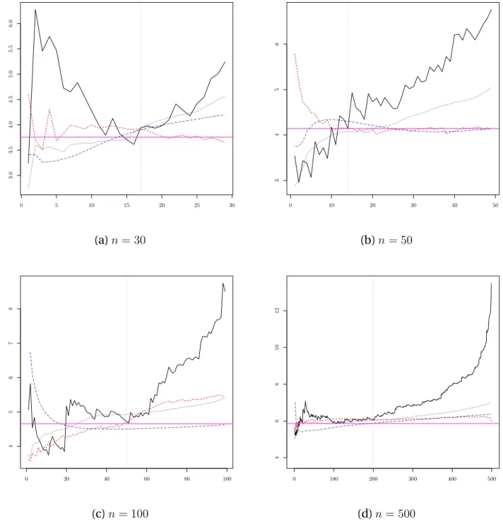
For each sample size and for each of the four distributions, we superimposed in Figure 2

253

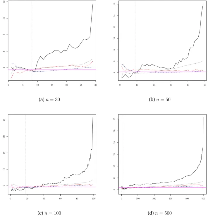
the mean estimators and the true theoretical quantile xpn, in Figure 3 the median estimators 254

and xpn and in Figure 4 the AMSE corresponding to estimators ˆx

W pn, ˆx WG pn , ˆx L pn and ˆx LG pn. For 255

visualization, we use a logarithmic scale in Figures 2 and 3. For each of the three Figures, we

256

have sixteen pictures that we numbered for clarity (i)–(xvi).

257

In the remainder of the paper, for the sake of simplicity, the symbols ↑ and ↓ are employed

258

to denote the expressions increases and decreases respectively. The discussion is done first

259

and foremost by distribution, afterwards by sample size if there is no redundancy. Otherwise

260

case are grouped.

261

Mean estimators

262

In Figure 2, except for the behavior of the mean estimators of ˆxL

pn when kn & n with n ≥ 50, 263 the graphs of ˆxW pn, ˆx WG pn , ˆx L pn, ˆx LG(1) pn and ˆx LG(2)

pn are convex. Except for the Pareto distribution 264

for which the slowly varying %(.) is constant, the simulations show that for the three other

265

distributions (Fréchet, Burr and Student) the bias of the extreme quantile estimators ↑ as the

266

sample size n ↑. This is due to the fact that the estimation of extreme quantiles of an order

267

(1 − 1/(5n)) is more difficult when n ↑. In other words, this phenomenon is a consequence

268

of 1/150 < 1/2500 which means that estimating x1/2500in Figures 2-(d) is more difficult than

269

estimating x1/150in Figures 2-(a).

270

For the distributions of Fréchet and Burr, the estimators ˆxW

pn, ˆx

WG pn and ˆx

L

pnhave high bias 271

for large values of the fraction sample kn. For large values of knthis bias ↑ as kn ↑ while, for

its small values this bias ↓ as kn ↑. We note a different behavior of the estimators ˆxLG(1)pn and 273

ˆ

xLG(2)pn : (1) for sample size n ∈ {30, 50}, the bias of these estimators ↓ as kn↑; (2) for n = 100,

274

this bias ↓ and becomes almost constant for large values of kn; (3) when n = 500, for small

275

values of knthe bias ↓ as kn↑ and for large values of knthe bias ↑ very slowly as kn↑.

276

Regarding the Student distribution, all estimators have high and ↑ bias for large values of

277

knwhatever the sample size. For very small values of kn, this bias ↓ as kn↑.

278

In addition, whatever the sample size and for each of the three distributions viz Fréchet,

279

Burr and Student, the bias of estimators ˆxWG

pn , ˆx L pn, ˆx LG(1) pn and ˆx LG(2)

pn becomes significantly less 280

important than the one of ˆxW

pnas kn↑. Given a sample fraction knnot too small, e.g. kn& 2n/5, 281

the simulations in Figure 2 show that, for the small sample sizes n ≤ 100, the bias of

estima-282 tors ˆxWG pn , ˆx L pn, ˆx LG(1) pn and ˆx LG(2)

pn is lower than the bias of Weissman estimator ˆx

W

pn. Thus, for 283

these three distributions, the estimators ˆxWG

pn , ˆx L pn, ˆx LG(1) pn and ˆx LG(2)

pn improve the bias of ˆxW_pn. 284

Regarding the Pareto distribution, since its slowly varying function %(.) is constant and

285

therefore its bias function b(.) ≡ 0 then, there is no asymptotic bias, i.e. the bias decreases

286

and becomes negligible as the sample size n and the fraction sample kn ↑. For small n, the

287

Weissman estimator seems to be better than the other estimators. Nevertheless, when the

288

sample size n ↑, all these estimators are approximately similar.

289

Median estimators

290

Generally, we observe from Figure 3 that the median estimators of ˆxWG

pn , ˆx L pn, ˆx LG(1) pn and ˆx LG(2) pn 291

are smooth and more stable than the Weissman estimator ˆxW

pn whatever the sample size. The 292

previous findings in Figure 2 on the bias of the estimators ˆxW pn, ˆx WG pn , ˆx L pn, ˆx LG(1) pn and ˆx LG(2) pn are 293

generally valid. Like the Weissman estimator ˆxW

pn, the other estimators have high variance for 294

small values of knand high bias for large values of kn. Indeed for the Fréchet, Burr and Student

295

distributions, if kn is large then the approximation %(.) is constant becomes worse and this

296

implies a high bias. Nevertheless, the bias of ˆxWG

pn , ˆx L pn, ˆx LG(1) pn and ˆx LG(2) pn is less significant 297 than ˆxW

pn. However for the Pareto distribution, the bias is negligible when knis large since %(.) 298

is constant. If knis small, one has too few observations, this implies then a high variance and

299

a small bias since one remains in the tail of the distribution.

300

AMSE

301

In Figure 4, for the four distributions we observe that AMSE(ˆxW

pn) is slightly less smooth than 302

those of its competing estimators. Except for AMSE(ˆxL

pn) when kn & n with n ≥ 50, the 303 graphs of AMSE(ˆxW pn), AMSE(ˆx WG pn ), AMSE(ˆx L pn), AMSE(ˆx LG(1) pn ) and AMSE(ˆx LG(2) pn ) are con-304

vex. The geometric shape of these graphs is similar to the ones in Figure 2. The AMSE of all

305

the estimators ↑ as the sample size n ↑ since the estimation of extreme quantiles of an order

306

(1 − 1/(5n)) is more difficult when n ↑.

307

For the Pareto distribution, AMSE of all the estimators ↓ as kn↑ and, when the sample size

308

n ↑ these AMSE are approximately similar for large values of kn. This can be explained by the

309

fact that there is no asymptotic bias. For this distribution, AMSE(ˆxWG

pn ) and AMSE(ˆx

W pn) are 310

approximately equal whatever kn and n. Moreover, AMSE(ˆxLG(1)pn ) seems to be higher than 311

the one of its competing estimators for the small sample sizes n ≤ 100.

312

Unlike the Pareto distribution, for the Student distribution AMSE of all the estimators ↑

313

as kn ↑. Moreover from a fraction sample kn not too small, AMSE(ˆxWpn) are clearly higher 314

than AMSE(ˆxWG

pn ) which is in turn higher than AMSE(ˆx

L

pn) which is finally itself higher than 315

AMSE(ˆxLG(1)pn ) and AMSE(ˆx

LG(2)

pn ). The two latter AMSE are approximately equal whatever kn 316

and n.

317

Regarding the Fréchet and Burr distributions, in general AMSE(ˆxW

pn) is higher than AMSE(ˆx

WG pn ), 318 AMSE(ˆxL pn) and AMSE(ˆx LG(2)

pn ) whatever the sample size. For small values of the fraction sam-319

ple, AMSE(ˆxW

pn) is smaller than AMSE(ˆx

LG(1)

pn ) and for large values of knthe opposite occurs, 320

i.e.AMSE(ˆxLG(1)pn ) < AMSE(ˆx

W

pn). Once the function AMSE reaches its minimum, we observe 321

that : (1) AMSE(ˆxLG(1)pn ) and AMSE(ˆx

LG(2)

pn ) ↑ slowly as kn ↑; (2) AMSE(ˆxWG_pn ) and AMSE(ˆx

L

pn)

322

↑ slightly faster as kn ↑; (3) AMSE(ˆxWpn) ↑ very faster as kn ↑. When the sample size n ↑, the 323

difference between AMSE(ˆxLG(1)

pn ) and AMSE(ˆx

LG(2)

pn ) ↓ as kn↑. 324

As by definition, AMSE is equal to the sum of the variance and squared bias of the esti-mator, i.e. AMSE(ˆx•_pn) = Avar(ˆx • pn) + ABias 2_(ˆx• pn), (22)

where letter “A” at the beginning of the notation refers to “asymptotic”, Figure 4 suggests the

325

following interpretations :

326

• The variance of estimators ˆxWGpn , ˆx

L

pn, ˆx

LG(1) pn and ˆx

LG(2)

pn seems smaller than the variance 327

of ˆxW

pn. The behaviour of the median estimators of ˆx

WG pn , ˆx L pn, ˆx LG(1) pn and ˆx LG(2) pn in Fig-328

ures 3 tend to confirm these statements. They are more stable than ˆxW pn. Notice that 329 the variance of ˆxW pn can be approximated by γ2 kn 6 1 + log26 kn npn 77

(see e.g. Beirlant et al.,

330

2004, p. 120).

331

• The standard deviation of the proposed estimators may be negligible compared to their

332

bias, i.e. Avar1/2_(ˆx•

pn) 0 ABias(ˆx

•

pn). Thus, since the bias of estimators ˆx

WG pn , ˆx L pn, ˆx LG(1) pn 333

and ˆxLG(2)pn are smaller than the bias of Weissman estimator ˆxW_pnat a scale factor to be de-334

termined, then AMSE(ˆxW

pn) is larger than AMSE(ˆx

WG pn ), AMSE(ˆx L pn), AMSE(ˆx LG(2) pn ) and, 335

from a sample fraction knnot too small AMSE(ˆxWGpn ) > AMSE(ˆx

LG(1)

pn ).

336

Choice of the optimal sample fraction

The proposed estimators depend on the fraction sample kn. Basically, the direct

minimiza-tion of the AMSE errors can be used as a criterion to select kn. However, this method can not

be considered in practice since the AMSE is unknown. A number of methods for the selec-tion of sample fracselec-tion kncan be found in Beirlant et al. (1996b); Drees and Kaufmann (1998);

Guillou and Hall (2001); Gomes and Oliveira (2001). Another option consists in choosing kn

corresponding to the range of stability of the estimators with respect to the fraction sample. In this study, one proposes to choose the largest integer knwhich minimizes a dissimilarity

measure between the four estimators ˆxW pn, ˆx WG pn , ˆx L pnand ˆx LG(2) pn , i.e. ˆ kn= arg min kn=1,...,n−1 :_; ;ˆxWpn− ˆx WG pn ; ;+ ; ;ˆxWpn− ˆx L pn ; ;+ ; ; ; ˆx W pn− ˆx LG(2) pn ; ; ; +; ;ˆxWG_pn − ˆx L pn ; ;+ ; ; ; ˆx WG pn − ˆx LG(2) pn ; ; ; + ; ; ; ˆx L pn− ˆx LG(2) pn ; ; ; < . (23)

This heuristic is used in non-parametric estimation. It relies on the idea that, if ˆknis

prop-337

erly chosen, all estimates should approximately give the same value. We refer to Gardes et al.

338

(2010) for an illustration of this procedure on simulated data. In addition, we illustrated, in

339

Figures 5 and 6, the dissimilarity procedure on the median estimators for N = 1000 simulated

340

samples from the Fréchet and Burr distributions respectively. In both Figures, the selected ˆkn

341

produce good results. Nevertheless, when selecting knindependently for each estimator,

bet-342

ter results may be produced as it is the case for instanceˆxL

pn in Figure 5-a and ˆx

W

pn in Figure 343

5-d. In the other Figures, the dissimilarity procedure performs as well as selecting kn

inde-344

pendently for each estimator by minimization of the error.

A brief summary

346

To summarize, these numerical experiments confirm that, for a large enough fraction sample

347

kn and large simple size (n > 100), ˆxLG(1)pn & ˆx

LG(2)

pn which means that it is reasonable to fix 348

fkn = 1. However, they show that the choice fkn = 1 is not optimal since ˆx

LG(2)

pn is better than 349

ˆ

xLG(1)pn in almost all cases, especially when n ≤ 100. Finally, despite the fact that we know there

350

is no optimal estimator for all cases, the simulations confirm that estimators ˆxWG

pn , ˆx

L

pn and

351

ˆ

xLG(2)pn are better than the Weissman estimator ˆx

W

pn especially for the bias and the AMSE for 352

the distributions where the function %(.) is not constant. The performance of all estimators

353

are approximately equal when %(.) is the constant.

354

5

Case study : estimation of high flood return period

355

In this section, we adapt and apply the proposed estimators to flood events. As illustrated

356

in 7, a flood event is mainly described with three variables obtained from a typical flood

hy-357

drograph. These variables are the flood peak (Q), flood volume (V ) and flood duration (D).

358

The data set used in this case study is taken from Yue et al. (1999) and consists in daily

nat-359

ural streamflow measurements from the Ashuapmushuan basin (reference number 061901).

360

The gauging station, located in the province of Quebec (Canada) is near the outlet of the

361

basin, at latitude 48.69◦_{N and longitude 72.49}◦_{W. In this region, floods are generally caused}

362

by high spring snowmelt. Data are available from 1963 to 1995. The flood annual

observa-363

tions of flood peaks, durations and volumes were extracted from a daily streamflow data set.

364

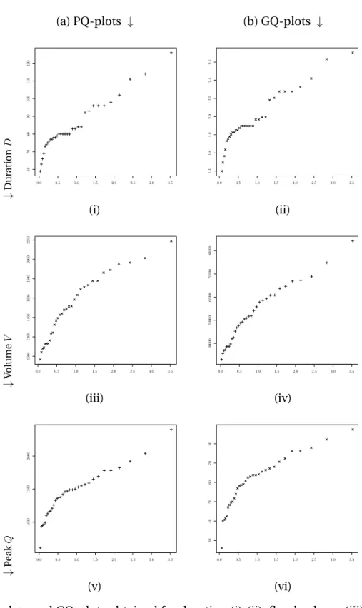
The proposed estimators of extreme quantiles are built by assuming that the CDF is heavy tailed. An exploratory study is performed using the PQ-plot in (6) and the GQ-plot in (7). Figures 8-a and 8-b illustrates respectively the PQ-plots and GQ-plots corresponding to three variables characterising the flood event. These plots show that the flood peak and the flood volume belong to the MDA(Fréchet). Indeed, for extreme points, the PQ-plots in Figure 8-(iii, v) seem to be approximatively linear and the GQ-plots in Figure 8-(iv, v) reveal a positive slope. On the other hand, the duration is not heavy-tailed since the curves of its PQ-plot in Figure 8-(i) and GP-plot in Figure 8-(ii) are approximately constant for extremes points. Thus, we are only interested in estimating of peak and volume. We considered the return period T ∈ {66, 99, 132, 165} years according to the sample size n = 33. Mathematically, the

problem is to estimate the quantile of order

(1 − p) ∈ {0.9848485, 0.989899, 0.9924242, 0.9939394}. For each T , the extreme quantile is estimated with ˆxW

p , ˆxLp, ˆxWGp and ˆx LG(2)

p . The fraction

365

sample on which the estimation is based was chosen by using criterion (23). For each value of

366

T , for each of the two selected variables (V and Q), we compute the mean and the standard

367

deviation (stdev) of the estimators. The estimated peaks and volumes are presented, with

368

their computed mean and standard deviation, in Table 2 and Table 3 respectively.

369

Unlike the stdev of the estimated volumes Table 3, we notice that the stdev of the

esti-370

mated peaks in Table 2 do not ↑ too fast as the return period T ↑. Also, stdev is large for the

371

estimated volumes. Thus, for this case study, the estimate of volume V deteriorates faster

372

than the estimate of the peak as T ↑. The estimation remains more stable when the extreme

373

quantile is not too far from the boundary of the sample, i.e. for a reasonable value of the

374

return period T . Indeed, estimation errors increase with the return period.

375

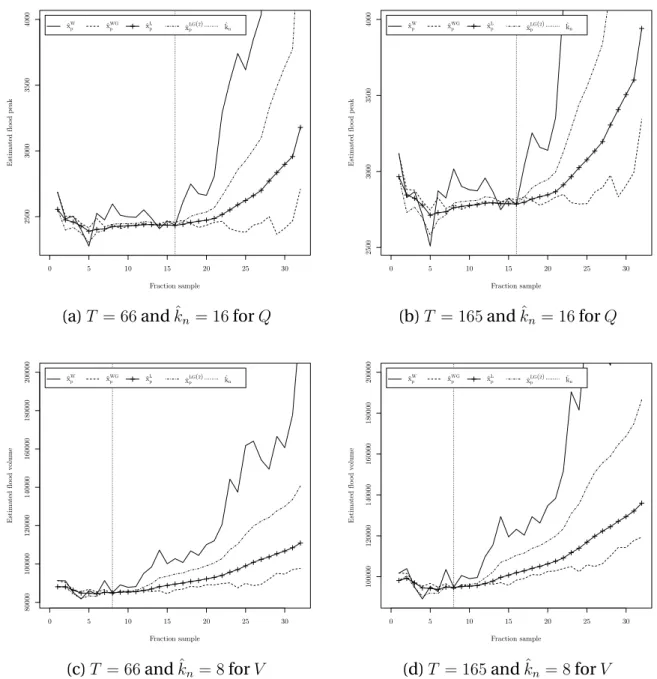
Figure 9 illustrates the selected fraction sample knand the estimators associated to each

376

one of the considered variables Q and V for the return periods T = 66 and T = 165 years.

377

For both variables of interest, we observe that the estimators ˆxL

p, ˆxWGp and ˆx LG(2)

p are smooth

378

and more stable compared to ˆxW

p . In addition, the difference between ˆxWp and the three other

379

estimators ↑ as the fraction sample kn↑. This indicates a high bias for large values of kn.

380

For Q series, criterion (23) suggests ˆkn = 16 respectively for T = 66 and T = 165 years.

381

Nevertheless, Figures 9-(a, b) show that we can choose ˆkn in the set {6, . . . , 16} where the

382

four estimators seem to have similar values. Moreover, for the estimator ˆxL

p, Figures 9-(a, b)

383

indicate that ˆkncan also be larger than 16 since this estimator is less sensitive to the selected

384

kn. ˆxWGp have a large volatility and for kn > 16 the difference between this estimator and

385

the other ones becomes important. Taking kn > 16 could lead to an overestimation of the

386

extreme quantiles.

387

Regarding the series of V , criterion (23) indicates that ˆkn = 8 is a good choice for T = 66

388

and T = 165 years. In Figures 9-(c, d), the observation of the range of stability of the four

389

estimators with respect to the fraction sample shows that ˆkn could be reasonably estimated

390

in {5, . . . , 10}. Figures 9-(c, d) confirm that ˆxL

p, ˆxWGp , ˆx

LG(2)

p are smooth and less sensitive

than ˆxW

p . Figure 9-(d) shows that one can build the estimator ˆxLp not only with the knlargest

392

observations but also with the entire sample, i.e. kn = n.

393

Even through the estimator values in Tables 2 and 3 are relatively similar, Figure 9

indi-394

cates that ˆxW

p is very sensitive to kn. Therefore, a bad choice of kncould lead to very different

395

estimator values whereas the other proposed estimators have a very small volatility with

re-396

spect to kn. Despite the fact that all the estimators are similar for a reasonable choice of kn,

397

the results of the case study suggest that it is advantageous to estimate extreme quantiles

398

with ˆxWG

p , ˆx

LG(2)

p and ˆxLp instead of ˆxWp . The case study results confirm the findings of the

399

simulation study, in particular the stability of the proposed estimators with respect to kn.

400

6

Conclusions

401

The present paper introduced (1) the geometric estimators of extreme quantiles and (2) a

402

“weighted” estimator of quantiles for high return periods T ≥ 2/(ne) where n is the

sam-403

ple size. Simulation results show that the proposed estimators given in (14), (19) and (20)

404

are smooth and more stable than the Weissman estimator (11). In addition, they improve

405

the bias. Since the accuracy of estimators depends on the precise choice of the number of

406

order statistics kn, a method of selection of kn is proposed and illustrated in the case study.

407

The case study shows that ˆxW

p is very sensitive to the selected knwhich is not the case of the

408

proposed estimators. Given the good performance of estimators (14), (19) and (20), we

pro-409

pose to explicit in future work, their asymptotic distributions. More precisely, we propose

410

to study asymptotic properties of the proposed estimators under less restrictive conditions

411

than those in Lekina (2010). This statistical result will allow, for instance, to build more

ac-412

curate estimation confidence intervals. In other respects, this result would allow to validate

413

the behaviour of the observed AMSE in the simulations and to identify the most efficient

es-414

timator. Finally, despite the fact that in EVA, it is often recommended to consider at the same

415

time several estimators of extreme quantiles since there is no optimal estimator for all cases,

416

according to the simulation results on simulated data in the present paper, we suggest to use

417

estimateur ˆxLG(2)p . Numerical experiments indicate that its AMSE is smaller than the one of

418

its competitors especially for the small samples i.e. n ≤ 100.

Acknowledgements

420

Financial support for this study was graciously provided by the Natural Sciences and

Engi-421

neering Research Council (NSERC) of Canada and the Canada Research Chair Program. The

422

authors wish to express their appreciation to the reviewers and the Editor-in-Chef for their

423

invaluable comments and suggestions.

424

References

425

Adamowski, K., Liang, G.-C., and Patry, G. G. (1998). Annual maxima and partial duration

426

flood series analysis by parametric and non-parametric methods. Hydrological Processes,

427

12(10-11):1685–1699.

428

Adlouni, S. E., Bobée, B., and Ouarda, T. (2008). On the tails of extreme event distributions in

429

hydrology. Journal of Hydrology, 355(1-4):16–33.

430

Apipattanavis, S., Rajagopalan, B., and Lall, U. (2010). Local polynomial-based flood

fre-431

quency estimator for mixed population. Journal of Hydrologic Engineering, 15(9):680–691.

432

Balkema, A. and de Haan, L. (1974). Residual life time at a great age. Annals of Probability,

433

2(5):792–804.

434

Beirlant, J., Broniatowski, M., Teugels, J. L., and Vynckier, P. (1995). The mean residual life

435

function at great age: Applications to tail estimation. Journal of Statistical Planning and

436

Inference, 45(1-2):21–48.

437

Beirlant, J., Dierckx, G., Guilllou, A., and Stˇaricˇa, C. (2002). On exponential representations of

438

log-spacings of extreme order statistics. Extremes, 5(2):157–180.

439

Beirlant, J., Dierckx, G., and Guillou, A. (2005). Estimation of the extreme value index and

440

regression on generalized quantile plots. Annals of Statistics, 11(6):949–970.

441

Beirlant, J., Goegebeur, Y., Teugels, J., and Segers, J. (2004). Statistics of extremes: theory and

442

applications. Wiley Series in Probability and Statistics. John Wiley and Sons.

443

Beirlant, J., Teugels, J., and Vynckier, P. (1996a). Practical analysis of extreme values. Leuven

444

University Press.

445

Beirlant, J., Vynckier, P., and Teugels, J. (1996b). Excess functions and estimation of the

ex-446

treme value index. Bernoulli, 2(4):293–318.

447

Bingham, N. H., Goldie, C. M., and Teugels, J. L. (1987). Regular Variation, volume 27.

Ency-448

clopedia of Mathematics and its Applications, Cambridge University Press.

Bobée, B., Cavadias, G., Ashkar, F., Bernier, J., and Rasmussen, P. (1993). Towards a systematic

450

approach to comparing distributions used in flood frequency analysis. Journal of

Hydrol-451

ogy, 142:121–136.

452

Breiman, L., Stone, C. J., and Kooperberg, C. (1990). Robust confidence bounds for extreme

453

upper quantiles. Journal of Statistical Computation and Simulation, 37(3–4):127–149.

454

Brunet-Moret, Y. (1969). Étude de quelques lois statistiques utilisées en hydrologie. Cahiers

455

d’hydrologie, 6(3).

456

Caeiro, F. and Gomes, M. (2006). A new class of estimators of a "scale" second order

parame-457

ter. Extremes, 9(3-4):193–211.

458

Caeiro, F., Gomes, M., and Rodrigues, L. (2009). Reduced-bias tail index estimators under a

459

third-order framework. Communications in Statistics - Theory and Methods, 38(7):1019–

460

1040.

461

Chebana, F., Adlouni, S., and Bobée, B. (2010). Mixed estimation methods for halphen

distri-462

butions with applications in extreme hydrologic events. Stochastic Environmental Research

463

and Risk Assessment, 24(3):359–376.

464

Chen, Y., Xu, S., Sha, Z., Pieter, V. G., and Sheng-Hua, G. (2004). Study on L-moment

esti-465

mations for log-normal distribution with historical flood data. International Association of

466

Hydrological Sciences, (289):107–113.

467

Coles, S. (2001). An introduction to statistical modeling of extreme values. Springer series in

468

statistics. Springer, 1 edition.

469

Daouia, A., Gardes, L., Girard, S., and Lekina, A. (2011). Kernel estimators of extreme level

470

curves. Test, 20(2):311–333.

471

de Haan, L. (1984). Slow variation and characterization of domains of attraction. In J. Tiago de

472

Oliveira, editor, Statistical Extremes and Applications, pages 31–48. Reidel, Dorchrecht.

473

de Haan, L. and Ferreira, A. (2006). Extreme Value Theory: An Introduction. Springer Series in

474

Operations Research and Financial Engineering.

475

de Haan, L. and Peng, L. (1998). Comparison of tail index estimators. Statistica Neerlandica,

476

52(1):60–70.

477

de Wet, T., Goegebeur, Y., and Guillou, A. (2012). Weighted moment estimators for the second

478

order scale parameter. Methodology and Computing in Applied Probability, 14:753–783.

479

Dekkers, A. and de Haan, L. (1989). On the estimation of the extreme value index and large

480

quantile estimation. Annals of Statistics, 17(4):1795–1832.

Diebolt, J., Gardes, L., Girard, S., and Guillou, A. (2008). Bias-reduced extreme quantiles

esti-482

mators of Weibull distributions. Journal of Statistical Planning and Inference, 138(5):1389–

483

1401.

484

Dierckx, G., Beirlant, J., Waal, D. D., and Guillou, A. (2009). A new estimation method for

485

Weibull-type tails based on the mean excess function. Journal of Statistical Planning and

486

Inference, 139(6):1905–1920.

487

Ditlevsen, O. (1994). Distribution arbitrariness in structural reliability. In G. Schueller, M.

Shi-488

nozuka, J. Y., editor, 6th International Conference on Structural Safety and Reliability, pages

489

1241–1247. Balkema, Rotterdam.

490

Drees, H. (1995). Refined Pickands estimator of the extreme value index. Annals of Statistics,

491

23(6):2059–2080.

492

Drees, H. and Kaufmann, E. (1998). Selecting the optimal sample fraction in univariate

ex-493

treme value estimation. Stochastic Processes and their Applications, 75(2):149–172.

494

Embrechts, P., Klüppelberg, C., and Mikosch, T. (1997). Modelling Extremal Events for

Insur-495

ance and Finance. Springer Verlag.

496

Falk, M. (1995). On testing the extreme value index via the Pot-method. Annals of Statistics,

497

23(6):2013–2035.

498

Feuerverger, A. and Hall, P. (1999). Estimating a tail exponent by modelling departure from a

499

Pareto distribution. Annals of Statistics, 27(2):760–781.

500

Fisher, R. and Tippet, L. (1928). Limiting forms of the frequency distribution of the largest or

501

smallest member of a sample. Proceedings of the Cambridge Philosophical Society, 24:180–

502

190.

503

Gardes, L., Girard, S., and Lekina, A. (2010). Functional nonparametric estimation of

condi-504

tional extreme quantiles. Journal of Multivariate Analysis, 101(2):419–433.

505

Girard, A., Guillou, A., and Stupfler, G. (2012). Estimating an endpoint with high order

mo-506

ments. Test. To appear.

507

Gnedenko, B. (1943). Sur la distribution limite du terme maximum d’une série aléatoire.

508

Annals of Mathematics, 44(3):423–453.

509

Goegebeur, Y., Beirlant, J., and de Wet, T. (2010). Kernel estimators for the second

or-510

der parameter in extreme value statistics. Journal of Statistical Planning and Inference,

511

140(9):2632–2652.

512

Gomes, M. I. and Oliveira, O. (2001). The bootstrap methodology in statistics of extremes:

513

theory and applications - choice of the optimal sample fraction. Extremes, 4(4):331–358.

Guida, M. and Longo, M. (1988). Estimation of probability tails based on generalized extreme

515

value distributions. Reliability Engineering and System Safety, 20(3):219–242.

516

Guillou, A. and Hall, P. (2001). A diagnostic for selecting the threshold in extreme value

anal-517

ysis. Journal of the Royal Statistical Society, Series B, 63(2):293–305.

518

Haddad, K. and Rahman, A. (2011). Selection of the best fit flood frequency distribution and

519

parameter estimation procedure: a case study for Tasmania in Australia. Stochastic

Envi-520

ronmental Research and Risk Assessment, 25(3):415–428.

521

Haeusler, E. and Teugels, J. (1985). On asymptotic normality of Hill’s estimator for the

expo-522

nent of regular variation. Annals of Statistics, 13(2):743–756.

523

Hall, P. and Park, B. U. (2002). New methods for bias correction at endpoints and boundaries.

524

Annals of Statistics, 30(5):1460–1479.

525

Hill, B. (1975). A simple general approach to inference about the tail of a distribution. Annals

526

of Statistics, 3(5):1163–1174.

527

Hosking, J. R. M. and Wallis, J. R. (1987). Parameter and quantile estimation for the

general-528

ized Pareto distribution. Technometrics, 29(3):339–1349.

529

Hosking, J. R. M., Wallis, J. R., and Wood, E. F. (1985). Estimation of the generalized

extreme-530

value distribution by the method of probability-weighted comments. Technometrics,

531

27(3):251–261.

532

Kratz, M. and Resnick, S. (1996). The QQ-estimator and heavy tails. Stochastic Models,

533

12(4):699–724.

534

Lall, U., il Moon, Y., and Bosworth, K. (1993). Kernel flood frequency estimators: Bandwidth

535

selection and kernel choice. Water Resources Research, 29(4).

536

Lang, M., Ouarda, T., and Bobée, B. (1999). Towards operational guidelines for over-threshold

537

modeling. Journal of Hydrology, 225(3–4):103–117.

538

Lekina, A. (2010). Estimation non-paramétrique des quantiles extrêmes conditionnels. PhD

539

thesis, Université de Grenoble.

540

Li, D. and Peng, L. (2009). Does bias reduction with external estimator of second order

param-541

eter work for endpoint? Journal of Statistical Planning and Inference, 139(6):1937–1952.

542

Moon, Y.-I. and Lall, U. (1994). Kernel quantite function estimator for flood frequency

analy-543

sis. Water Resources Research, 30(11).

544

Ouarda, T. B., Girard, C., Cavadias, G. S., and Bobée, B. (2001). Regional flood frequency

545

estimation with canonical correlation analysis. Journal of Hydrology, 254(1–4):157–173.

Pickands, J. (1975). Statistical inference using extreme order statistics. Annals of Statistics,

547

3(1):119–131.

548

Prescott, P. and Walden, A. T. (1980). Maximum likelihood estimation of the parameters of

549

generalized extreme-value distribution. Biometrika, 67(3):723–724.

550

Quintela-del-Río, A. and Francisco-Fernández, M. (2011). Analysis of high level ozone

con-551

centrations using nonparametric methods. Science of The Total Environment, 409(6):1123–

552

1133.

553

Rényi, A. (1953). On the theory of order statistics. Acta Mathematica Hungarica, 4(3–4):191–

554

231.

555

Rosen, O. and Weissman, I. (1996). Comparison of estimation methods in extreme value

556

theory. Communication in Statistics-Theory and Methods, 24(4):759–773.

557

Salvadori, G., De Michele, C., Kottegoda, N. T., and Rosso, R. (2007). Extremes in Nature: An

558

Approach Using Copulas. Springer.

559

Schultze, J. and Steinebach, J. (1996). On least squares estimates of an exponential tail

coef-560

ficient. Statistics and Decisions, 14(3):353–372.

561

Smith, J. (1987). Estimating the upper tail of flood frequency distributions. Water Resources

562

Research, 23(8):1657–1666.

563

Smith, R. L. (1985). Maximum likelihood estimation in a class of nonregular cases.

564

Biometrika, 72(1):67–92.

565

Smith, R. L. (1986). Extreme value theory based on the r largest annual events. Journal of

566

Hydrology, 86(1-2):27 – 43.

567

Stedinger, J. R. (2000). Flood frequency analysis and statistical estimation of flood risk. In

568

Inland Flood Hazards : Human, Riparian and Aquatic Communities, chapter 12, pages

569

334–358.

570

Tsourti, Z. and Panaretos, J. (2001). A simulation study on the performance of extreme-value

571

index estimators and proposed robustifying modifications. 5th Hellenic European

Confer-572

ence on Computer Mathematics and its Applications, Athens, Greece, 2:847–852.

573

Weissman, I. (1978). Estimation of parameters and large quantiles based on the k-largest

574

observations. Journal of the American Statistical Association, 73(364):812–815.

575

Willems, P., Guillou, A., and Beirlant, J. (2007). Bias correction in hydrologic GPD based

ex-576

treme value analysis by means of a slowly varying function. Journal of Hydrology, 338(3–

577

4):221–236.

Young-Il, M., Lall, U., and Bosworth, K. (1993). A comparison of tail probability estimators

579

for flood frequency analysis. Journal of Hydrology, 151(2-4):343 – 363.

580

Yue, S., Ouarda, T., Bobée, B., Legendre, P., and Bruneau, P. (1999). The Gumbel mixed model

581

for flood frequency analysis. Journal of Hydrology, 226(1-2):88–100.

Distribution Density Sequences Normal f (x) = √1 2πexp * −1 2x 2 + an = (2 log n)−1/2 x ∈ R bn = (2 log n)1/2−

log log n + log 4π

2 (2 log n)1/2 Exponential f(x) = λ exp(−λx) an = 1/λ x ≥ 0 bn = log (n)/λ Cauchy f (x) = 1 π 1 1 + x2 an = 0 x ∈ R bn = n/π Beta f (x) = Γ(a + b) Γ(a)Γ(b)x a−1 (1 − x)b−1 an = * n Γ(a + b) Γ(a)Γ(b + 1) +−1/b 0 < x < 1, a, b > 0 bn = 1

Table 1: Limited number of examples of the theoretical normalized sequences anet bn.

!! !! !!!! !! !!! !!!!! Estimator Return period T 66 99 132 165 ˆ xW 1/T 2435.00 2583.10 2693.62 2782.58 ˆ xL 1/T 2456.14 2607.50 2720.55 2811.61 ˆ xWG 1/T 2433.15 2583.25 2695.34 2785.62 ˆ xLG(2)_1/T 2432.61 2584.59 2698.14 2789.64 mean 2439.45 2590.01 2702.45 2793.02 stdev 11.22 11.68 12.13 12.55

Table 2: Estimated flood peak Q.

!!! !!! !!! !!! !! !!!! Estimator Return period T 66 99 132 165 ˆ xW 1/T 84979.31 89238.64 92389.53 94909.97 ˆ xW 1/T 84267.36 88418.86 91485.84 93937.06 ˆ xWG 1/T 84970.60 89146.48 92233.20 94700.84 ˆ xLG(2)_1/T 84761.40 88953.95 92053.78 94532.40 mean 84957.27 89158.70 92264.57 94747.80 stdev 652.10 708.26 751.46 786.86

0 100 200 300 400 500 0 5 10 15 20 25 sample size quan tile xp Xi 0 100 200 300 400 500 0 5 10 15 20 25 sample size quan tile xp Xi (a)T = 25 (b)T = 250 0 100 200 300 400 500 0 5 10 15 20 25 sample size quan tile xp Xi (c)T = 600

Figure 1: Difference between large quantiles within and outside the sample. Scatter plot of the

Fréchet distributed sample {Xi, i = 1, . . . , 500} (× × ×) with tail index γ = 0.5, location

param-eter m = 0 and scale paramparam-eter s = 1, the extreme quantile xp(− − −) and observations higher