Efficient stability analysis of flows using complex mapping techniques

OATAO is an open access repository that collects the work of Toulouse

researchers and makes it freely available over the web where possible

Any correspondence concerning this service should be sent

to the repository administrator:

tech-oatao@listes-diff.inp-toulouse.fr

This is an author’s version published in:

http://oatao.univ-toulouse.fr/25

923

To cite this version:

Sierra Ausin, Javier

and Fabre, David

and Citro, Vincenzo

Efficient stability analysis of flows using complex mapping

techniques.

(2020) Computer Physics Communications, 251.

107100. ISSN 0010-4655 .

Official URL:

https://doi.org/10.1016/j.cpc.2019.107100

Efficient stability analysis of fluid flows using complex mapping

techniques

*

Javier Sierra

a,b,*,

David

Fabre

a,

Vincenzo Citro

b •1MFT, UPS, Allée du Professeur Camille Soula, 31400 Toulouse, France b DIIN, University of Sa/emo, 84084 Fisdano, /ta/y

ABSTRACT

Keywords:

Linear scabilicy analysis Linear acouscics

Non-reneccing boundary conditions

Global linear stability analysis of open flows leads to difficulties associated to boundaiy conditions, leading to either spurious wave reflections (in compressible cases) or to non-local feedback due to the elliptic nature of the pressure equation (in incompressible cases). A nove( approach is introduced to address both these problems. The approach consists of solving the problem using a complex mapping of the spatial coordinates, in a way that can be directly applicable in an existing code without any additional auxiliaiy variable. The efficiency of the method is first demonstrated for a simple 1D equation modeling incompressible Navier-Stokes, and for a linear acoustics problem. The application to full linearized Navier-Stokes equation is then discussed. A criterion on how to select the parameters of the mapping function is derived by analyzing the effect of the mapping on plane wave solutions. Finally, the method is demonstrated for three application cases, including an incompressible jet, a compressible hole-tone configuration and the flow past an airfoil. The examples allow to show that the method allows to suppress the artificial modes which otherwise dominate the spectrum and can possibly hide the physical modes. Finally, it is shown that the method is still efficient for small truncated domains, even in cases where the computational domain is comparable to the dominant wavelength.

1. Introduction

Numerical simulations of real flow configurations in open domains require artificial boundary conditions to allow vortical structures to freely escape from the domain and avoid wave re­ flections. The most common Artificial Boundary Conditions (here denoted as ABC) chosen for compressible fluid flows are the

sponge

regions which imply the introduction of an artificial damp­ ing term in an outer 'sponge layer' located far away from the interesting regions. The main advantage of this method is its simplicity. However, it generally leads to extremely large meshes characterized by sponge layers much larger than the regions of interest. An alternative method is the Perfectly Matched Layer (PML) treatment of ABCs. First introduced by Berenger (1) for electromagnetic radiation problems and later extended for lin­ ear acoustics problems by Bermudez et al. (2), this method has proven its efficiency for studying compressible flows using lin­ earized Navier-Stokes Equations (LNSE) in the frequency do­ main. However, since the method introduces a spatial attenuation

*

The review of Chis paper was arranged by Prof. N.S. Scocc.

* Corresponding auchor ac: lMFT, UPS, Allée du Professeur Camille Soula, 31400 Toulouse, France.

E-mail address: javier.sierra@imft.fr u. Sierra).

which depends upon the frequency, it cannot be directly applied to global stability problems where the frequency is unknown. A possible solution is to introduce auxiliary variables in the buffer region leading to a formulation where the dependency with re­ spect to the frequency does not appear anymore, as done for instance by Hu et al. (3) and Whitney (4). However the introduc­ tion of these new variables significantly increases the dimension of the problems under investigation. As well, in the formulation of PML the estimation of a base state is required, which is not generally an easy task for flows with domains whose geometry is convoluted.

ABC are also required for the stability analysis of purely in­ compressible open configurations such as swirling flows (see [SI). The difficulties are due to the strong convective amplification of vortical perturbations, which may still be active at the ourlet boundary, and to the elliptic nature of the pressure equation leading to nonlocal feedback between upstream and downstream boundary conditions. Lesshaft (6) showed that these two prob­ lems lead to the existence of two families of artificial eigenmodes which can in some situations dominate the spectrum and hide the physically relevant modes. Fabre et al. (7) observed similar difficulties in studying the response to harmonie forcing of a jet flow through a zero-thickness circular hole. ln this work, the authors introduced a method based on the Complex Mapping

(CM) of the spatial coordinates. The key idea is to introduce a spatial damping which is independent upon the frequency and thus directly fitted to eigenvalue computations. In a subsequent work Fabre et al. [8], the method was successfully applied to the eigenvalue analysis of the jet through a circular hole of nonzero thickness, allowing to capture unstable global modes arising from the existence of a recirculation region within the thickness of the hole.

The purpose of this work is to explain the principle of the CM technique and to show that is applicable to the linear sta-bility analysis of both compressible and incompressible flows. We demonstrate that (i) it is efficient as a non-reflexion con-dition for acoustic perturbations and (ii) it is able to provide a sufficient decay for the large convective amplification of vortical perturbations, thus efficiently fixing both problems identified above.

The remainder of the paper is organized as follows: In Section 2we introduce the complex mapping methodology for a linear PDE problem and we draw some parallels between CM and PML. In Section 3we apply CM to a canonical scalar PDE problem, the Ginzburg–Landau equation. This toy model serves to demonstrate how CM can be used to reduce non-local effects, i.e. to suppress the (elliptic) feedback pressure mechanism in the incompressible Navier–Stokes equations. In Section 4 we discuss the effect of CM on the spectrum of the Helmholtz equation that governs inviscid linear acoustics, showing that the methods effectively work as a non-reflective boundary condition. Sections5and6focus on the application of complex mapping to Navier–Stokes equations. We first review the concept of global stability of both incompressible and compressible flows, which motivates the study of the effect of CM in plane acoustic and hydrodynamic waves. Finally, in Section 6 three application cases, where CM is used for stability computations, are presented. First an incompressible jet flow which suffers from non-local feedback due to strong spatial amplification of linear perturba-tions. ABC are mandatory in this case to correctly characterize the spectrum of the linear problem. Second, we study the effect of CM in a compressible flow, the hole-tone configuration, by looking at the performances of CM with respect to sponge layers. The last numerical case is the weakly compressible flow past a symmetric airfoil at a large angle of attack. In this last test case, it is shown that complex mapping region is still effective even when its length is shorter than the acoustic wavelength. The Navier–Stokes and linear acoustics computations are performed using the FreeFem++ solvers and Octave/Matlab drivers provided by the StabFem suite (see the review paper by Fabre et al. [9] for details). Programs reproducing most of the figures of the paper are available online on the web page of the project (https: //gitlab.com/stabfem/StabFem).

2. Introduction of the complex mapping technique for eigen-value problems

2.1. Mathematical framework (1D case)

To introduce the method, let us first consider for simplicity a one dimensional autonomous linear partial differential equation (PDE) with the following form:

∂

Ψ

∂

t

=

LΨ (1)

whereΨ(x

,

t) is defined on the domain x

∈

Ω

= [

0

, ∞]

, andL is a linear operator. The asymptotic linear stability of such PDE is driven by modal solutions with the form

Ψ(x

,

t)

= ˆ

Ψ(x)e−iωt (2)

where

ω

is the complex eigenvalue. We are therefore led to a linear eigenvalue problem with the form

−

i

ω

Ψ

=

LΨ

.

(3)

The problem is then said to be linearly unstable if there exists at least one eigenvalue such as

ωi

>

0. Note that the modal ansatz

(2)is also at the basis of the so-called frequency-domain approach to harmonically forced non-homogeneous PDEs (such as wave scattering problems). The difference is that in the frequency-domain approach it is sufficient to consider the solution for real values of the frequency

ω

, while in the linear stability approach

ω

has generally to be solved as a complex number.

2.2. Motivation of the complex mapping

The difficulty we want to solve is associated to the existence of solutions behaving asΨ(x

,

t)

≈

eikx−iωt _{as x}

_{→ ∞}

_{, which,}

according to the argument of k, may be oscillating, or even worse, exponentially growing. The idea is to consider an analytical con-tinuation of the solution for complex x, and solve in a region of the complex plane where all physically relevant solutions are nicely decaying. To this aim, we will define a mapping from a (real) numerical coordinate X defined in a truncated domain X

∈

[

0

,

Xmax

]

to the physical coordinate x.

2.3. Definition of a smooth mapping

The application of the proposed method to a given problem leads to two separate regions: (i) an unmodified domain for X

<

X0 and (ii) a mapped region for X

>

X0, characterized by a

parameter

γc

defining the direction in the complex plane. The simplest choice is as follows:

x

=

G_x(X )

=

{

X for X

<

X0,

[

1

+

i

γc

]

X for X

>

X0, (4)

which transforms the x-derivatives as follows:

∂

∂

x

=

⎧

⎪

⎨

⎪

⎩

∂

∂

X for X

<

X0, 1 1

+

i

γc

∂

∂

X for X

>

X0, (5)

In practice it is desirable to design a mapping function which gradually enters into the complex plane with a transition region of characteristic length Lc, in order to avoid possible reflections

caused by an abrupt change at X

=

X0. This can be achieved using

a mapping function with the form: G_x

:

_R

→

_C such that x

=

G_x(X )

=

[

1

+

i

γc

g(X )

]

X (6) where g(X ) has to be chosen as a smooth function such as g(X )

=

0 for X

<

X0and g(X )

≈

1 for X

>

X0

+

Lcup to Xmaxfor a length

LCM

=

Xmax

−

(

X0

+

Lc

)

where complex mapping is activated. We found good performance using g(X )

=

tanh

(

[

X−X0 Lc

]2

)

. To apply the method to a linear PDE of the form(3), one has simply to modify the spatial derivatives as follows:

∂

∂

x

≡

Hx

∂

∂

X with Hx(X )

=

(

∂

Gx

∂

X

)

−1

.

(7)

For a given PDE problem, complex mapping function g

∈

Cr(Ω), where r is equal to the highest derivative order of the considered PDE problem. This requirement is due to the fact that the deriva-tive should be continuous between the physical and the complex mapping domain to avoid any numerical reflection.

Fig. 1. Numerical spectrum of the Ginzburg Landau equation (a) without and (b) with complex mapping, for domain size Xmax=40 (red crosses), Xmax=20 (blue squares) and Xmax=15 (green circles). The theoretical solution in infinite domain in absence of non-local feedback is displayed by black dots (discrete spectrum) and black dotted line (essential spectrum).

2.4. Comparison with the perfectly matched layer method

The CM method introduced here shares similarities with the PML technique. The PML technique was first introduced by Be-ranger in the context of electromagnetic waves (Maxwell equa-tions). The initial exposition of the method was formulated in the temporal domain and involved the introduction of auxiliary vari-ables. Soon after, the method was reformulated in the frequency domain (i.e. considering solutions with modal temporal depen-dance e−iωt) by Teixeira [10] who showed that it is equivalent to modifying the spatial derivative operators as follows :

∂

∂

x

→

1 1

+

iσ_ω(x)

∂

∂

x

.

(8)

Teixeira & Chew [10] also pointed out that this reformula-tion is equivalent to solving for a complex variable defined as follows: x

=

GPML(X )

=

X

+

i

ω

∫

X

σ

(X′)dX′

.

(9)

Comparing these equations with the ones defining our com-plex mapping, we immediately see that the two methods are closely related, the difference being that in the PML the coor-dinate mapping depends upon the frequency

ω

. Therefore, the method is not directly applicable to eigenvalue problems, where

ω

is unknown.

3. Application to a 1D model problem

3.1. Description of the model and theoretical solution

In this section we first demonstrate the efficiency of the method for a one dimensional PDE which has often been used as a model for global hydrodynamical instability of open shear flow, namely the linear Ginzburg–Landau equation (see the recent book of Schneider & Uecker [11, Ch. 10] for a rigorous mathematical derivation and analysis of this equation):

−

i

ω

Ψ

= −

U

∂

Ψ

∂

x

+

κ

∂

2_Ψ

∂

x2

+

µ

(x)Ψ

+

F(

ψ

)

.

(10)

In this model, U represents the convective velocity,

κ

a diffusion coefficient,

µ

(x) a local growth rate of the instability,F a non-local coupling term. We use the following law for the non-local growth rate:

µ

(x)

=

µ

∞

+

µ1

e −x/L∗

.

(11)

where

µ

∞

, µ1,

L∗

∈

R are parameters of the problem. With this choice, the homogeneous problem in a semi-infinite domain (without the term F) admits a discrete spectrum

ωn

with n

=

1

,

2

, . . .

(where the linear operator is Fredholm and closed, that is the solution belongs to the space, here H1

0(R

+

)). Discrete modes are alike to eigenvalues in finite dimensional problems. The spec-trum of Eq. (10)is also composed of a second set, denoted as

essential spectrum

ωess

(

ℓ

) with

ℓ ∈

_{R (where the linear operator is} no longer Fredholm or closed, for more details on the spectrum of infinite dimensional operators see the book of Kapitula & Promislow [12, Ch. 3]). This set depends uniquely on asymptotic coefficients of Eq. (10). The corresponding solution is given in

Appendix A ( Eq.(35)and Eq.(37)). Following Lesshafft [6], we introduce a nonlocal feedback term defined as

F(

ψ

)

=

ϵ

e−

(x−_xA)2

b2 Ψ_{(xS) (12)}

where

ϵ

is a coupling parameter, xS is the location of a ‘‘sensor’’

(located close to the outlet) and xA the location of an activator

(located close to the inlet). Such a feedback exists in real flows through the pressure, either as a result of backward-propagating pressure waves (in compressible flows) or as an instantaneous non-local effect (in incompressible flows). Lesshaft [6] showed that this nonlocal term leads to the appearance of a family of artificial eigenmodes called ‘‘arc branch modes’’ which are clearly dependent on the size of the domain and hence have to be ruled out when one wants to focus on the discrete modes. We will show that the complex mapping technique efficiently reaches this objective.

3.2. Numerical solution and effect of CM

In this section, we assume the following values for the model parameters:

µ

∞

= −

1,

µ1

=

10,

κ =

1

−

i, U

=

6

.

5 and

L∗

₌

10. With this choice, the problem is absolutely unstable in the range x

∈ [

0

,

4

.

6

]

, convectively unstable in the range

x

∈ [

4

.

6

,

23

]

, and locally stable for x

∈ [

23

, ∞]

. Moreover, the analytical solution (see Appendix A) tells us that the two first modes of the discrete spectrum are unstable while the higher-order discrete eigenvalues and the essential spectrum are stable. In the following we will consider the numerical solution of the problem using a feedback term with parameters xA

=

1, b

=

0

.

2,

xB

=

Xmax

−

1,

ϵ =

0

.

1. The numerical solution is done using a

Chebyshev collocation method.

Fig. 1(a) displays the numerically computed spectra without complex mapping (x

≡

X ) for three values of the numerical

domain size, namely Xmax

=

15

,

20 and 40. In all cases, the

numerically computed spectra are dominated by the ‘‘arc-branch’’ artificial modes whose location clearly depends upon the size of the domain. Note that with the chosen parameters, the arclength modes are located in the unstable (

ωi

>

0) half-plane. For the smallest domains (Xmax

=

15 and 20) these modes completely

mask the physically relevant discrete modes. Computing the most unstable mode is only possible with the largest domain (Xmax

=

20), and yet some mismatch with the theoretical solution can be observed on the figure. Fig. 1(b) displays the numerically computed spectra using the complex mapping technique, with the same values of the numerical domain size (Xmax

=

15

,

20

and 40), and applying the complex mapping starting from L0

=

Xmax

−

5. The other parameters affecting the complex mapping

are

γc

=

10 and Lc

=

1.

As one can observe, the introduction of CM has the effect of completely suppressing the arc-branch of artificial modes, and for all cases the two unstable discrete eigenvalues (plus two stable ones) are correctly recovered. One still observes a branch of artificial eigenvalues, but they are rejected far away from the unstable region, and below the theoretical essential spectrum. It is remarkable that the CM technique allows to correctly compute the unstable discrete modes independently of the size of the domain, even in the two smallest cases (Xmax

=

15, Xmax

=

20)

where the problem remains convectively unstable at the location of the numerical truncation.

4. Application to linear acoustics

4.1. Physical problem and asymptotic solution

In this section, we demonstrate the efficiency of the complex mapping method for a purely linear acoustic wave problem, cor-responding to a cylindrical pipe of radiusD₂ and length L opening to a semi-infinite domain. This is a classical problem in linear acoustics, the interested reader is referred to the book of Fletcher & Rossing [13, Ch. 8] for a brief review.

In an inviscid framework, it is classical to express the velocity and pressure in terms of the velocity potential Φ, namely u

=

∇

Φ, p

=

ρ

∂Φ_∂

t. The problem reduces to the Helmholtz equation:

∇

2Φ

+

(

ω

c∞

)2

Φ

=

0 in Ω (13)

where c∞is the speed of sound. Eq.(13)is complemented with boundary conditions. At the walls, the bottom and the axis we impose non-penetration conditions:

∇

Φ

·

n

=

0 at Γin,Γ_wall,Γa (14)

In addition, in an unbounded space, the relevant asymptotic condition is the Sommerfeld condition (see the review of Schot [14]):

∂

Φ

∂

rs

−

(

i

ω

c∞Φ

+

Φ rs

)

→

0 as rs

=

√

r2

₊

_z2

_{→ ∞}

₍₁₅₎

Physically this condition means that away from the outlet, the acoustic field matches with a monopolar source leaving the domain, and there is no wave coming from infinity. In practice, when working with a truncated domain, this asymptotic condi-tion has to be replaced by an artificial boundary condicondi-tion at the outlet surfaceΓoutwhich does not lead to any notable reflection.

We will show in the next subsection that the use of CM efficiently fulfills this goal. Note that the physical problem considered here admits an analytical solution in the limit of long pipes (L

/

D

≫

1). This solution is obtained by matching a plane-wave description within the pipe to a monopolar radiation in the outer domain, and details are given in Appendix B. The corresponding result is as follows:

ω ≈

(n

−

1

/

2)

π

c∞ L

+

∆

−

i

π

2 32 (2n

−

1)2c∞D2 (L

+

∆)3 with n

=

1

,

2

, . . .

(16)

where∆

=

4D

/

3

π

is the so-called correction length [13]. The first term in this expression means that the acoustical wavelength

λac

=

2

π

c∞

/ωr

is 4

/

(2n

−

1) times the effective length (L

+

∆) of the pipe, which corresponds to the resonance condition of an ideally open pipe. The second term represents the damping rate due to radiation in the semi-infinite space, which is found to be largest for higher-order modes. In addition, the physical problem in infinite domain admits an essential spectrum whose outer boundary, the Fredholm border (FB), is located on the real

ω

-axis, corresponding to weak solutions of the problem which are not square-integrable and do not satisfy the Sommerfeld condition, and defined as:

ωFB

=

c∞

ℓ,

for

ℓ ∈

_R (17)

Physically, these solutions correspond to plane waves coming from infinity and reflecting along the wall (with weak influence of the pipe).

4.2. Numerical results

In this section we present results obtained using the CM method. Technically, the method was used by applying the map-ping equation(6)to both r and z coordinates, namely r

=

G(R) and z

=

G(Z ) where R

,

Z are the numerical coordinates in the

truncated domainΩ. Hence, both r and z derivatives appearing in the Laplacian operator are modified using Eq. (7). We apply the mapping outside of the box (R

,

Z )

=

[

0

,

R0

] × [−

H

,

Z0

]

(corresponding to the dashed box inFig. 2).

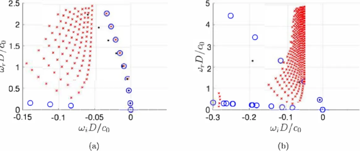
Fig. 3displays the computed spectra for a long and a short pipe, respectively L

/

D

=

10 and L

/

D

=

3. The results of the CM method are compared to a reference solution using a much larger domain (Rmax

=

50) and imposing directly the Sommerfeld

boundary condition at the outlet (seeAppendix Cfor details about implementation of this case). For the longest pipe, the both the CM method and the reference case allow to compute accurately the discrete spectrum (8 discrete modes can be found in the range displayed in the figure). In the reference case without CM, the numerically computed spectrum also contains a large number of artificial eigenvalues, all located in the stable range (

ωi

< −

0

.

05), which correspond a discretized version of the essential spectrum discussed above.

For the physical modes, the numerical results fit well with the asymptotic formula equation(16)for the lowest modes. For the higher frequency modes the asymptotic formula overpredicts the damping; this is not surprising since the asymptotic theory assumes monopolar radiation while high frequency modes are known to be more directive, hence less energy is radiated.

For the shortest pipe (Fig. 3(b)), the discrete modes are much more damped. As one can observe, the computation without CM only allows to compute the first mode of the series. All the others are located in the region occupied by the artificial modes, leading to the impossibility to compute them. Note that the agreement with the asymptotic formula equation(16)is less good than for the long pipe because the hypothesis L

/

D

≫

1 does not hold. Considering the second mode, the pressure component along the axis for L

/

D

=

3 is reported inFig. 2(b). The pressure field in the physical case (without CM) is approximately a standing wave within the pipe (with real and imaginary parts in phase) and an outward propagating wave outside of the pipe (with a

π/

2 phase shift). As can be seen, use of the CM leaves the pressure field unaffected within the pipe and up to z

=

Z0, but the structure

is completely damped for farther distances.

As for the artificial eigenvalues, using the CM technique has the effect of ‘sweeping’ them towards much larger damping rates, and allows to correctly compute the 6 first modes of the series. Moreover, it can be seen that the imposition of the CM method

0.05

�

0

-0.05

0.05

rwall

0

ZL

_r

_:D/2

L

�

-0.05

....

-10

0

10

20

rin

_z

(a)

(b)

Fig. 2. (a) Sketch or the now configuration representing the now through the acoustic circuit. Geometric paramerers are displayed. (b) Evolution or acoustic waves along the z-direcrion at the axis for the short pipe (L/D

=

3). Real and imaginary parts or the pressure componenr or the Jeading mode (see Fig. 3 (b)) are depicted. Solid line corresponds ro CM and dashed-dotted (red online) ro Sommerfeld boundary condition. (For inrerpretation or the rererenœs ro color in this figure legend, the reader is rererred ro the web version or this article.)

2.5

2

�1.5 Ci

3 1

0.5

₀

0

0 0 o

o�--�-�-�--

--

----o.1s -0.1

-0.05

wiD/co

(a)

0

5

4

. .

0

0

0

5

_{croo oo}

0

0 �--�--��...,_ __ ...,.. __ _ -0.3 -0.2 -0.1

wiD/co

(b)

0

Fig. 3. Acoustic specrrum or the open-pipe configuration for (a) a long pipe (l/D

=

10) and (b) a short pipe (L/D

=

3). Blue circles correspond ro result using CM

(with parameters Xo

=

Zo

=

2, �

=

2, Yc

=

1 and domain size Rou,

=

10), and red crosses to a rererence solution using a much larger domain (Rmœc

=

50) and

Sommerfeld boundary condition at the ourlet. Black dots correspond ro the asymprotic formula equation (16).

dramatically affects their location in the complex plane. Mathe­

matical analysis if the essential spectrum shows that the effect of

CM is to 'tilt' it from the real axis (as defined by

(

1

7)

) to a line in

the complex plane defined by

WfB

=

C

oo

l--1-. -

₁

=

ic

oo

le

-iarcran(ycl

, for

lE

JR

.

+1yc

(18)

The artificial modes obtained with CM are obseived to lie approx­

imately along this line.

Note that in addition to be more accurate with shorter do­

mains, the CM is numerically less demanding than the Sommer­

feld method. ln elfect, as the eigenvalue appears only as

w2,

it is

enough to formulate the problem for <I> and solve for w

2•

On the

other hand, using Sommerfeld method, as the eigenvalue appears

as

w2

_{in the Helmholtz equation and}

_w

_{in the boundary condition,}

it is required to solve for an augmented state vector [ <I>,

<l>i]

with

</>1

=

w<I>. The corresponding formulation is detailed in

Appendix C.

To investigate the performance of the CM method, we display

in

Table 1

the numerical values of the three first eigenvalues

of the short pipe (with L/D

=

3) for various choices of the

domain size

Raut

and complex mapping parameters r

0,

z

0, Le and

Yc·

We note that the results agree within 1% . Considering that

the acoustic wavelength of the first mode is

Àac �

2:,r /

w1,, �

13.7, it is specially remarkable that the CM method is able to

produce accurate result with a domain as short as Rout

=

5, which

represents a fraction of this wavelength.

5. Application

to

global srability anatysis

5.1. Governing equations

Let us consider both compressible or incompressible Navier­

Stokes equations written in compact operator form as

ôq(x·

t)

B--'-

=

NS(q(x; t)).

ôt

(19)

Here q denotes the state vector defined as q

=

[u; p;

T; p) using

non-conseivative variables for compressible or

q

=

[u; p) for

incompressible flows.

B

is a linear operator specifying how the

time derivative applies to variables. Finally,

NS

is the nonlinear

Navier-Stokes operator. A detailed form of the compressible op­

erator is given by Fani et al. (

15

) and the incompressible case is

detailed in the review article of Fabre et al. (

9

). ln the following

sections, Reynolds number is defined as Re

=

U,Lr

where L,,

U,

are the characteristic length and velocity scate"f of the flow

Table 1

Eigenvalues of a short open pipe (L/D = 3) for various choices of the complex-mapping parameters.

Rout r0 z0 Lc γc ω1 ω2 ω3

20 2 2 1 1 0.4623−0.0076i 1.4089−0.0560i 2.3894−0.1197i

10 2 2 1 1 0.4624−0.0076i 1.4091−0.0560i 2.3898−0.1200i

5 2 2 1 1 0.4639−0.0061i 1.4085−0.0561i 2.3895−0.1199i

10 2 2 1 0.2 0.4624−0.0076i 1.4091−0.0560i 2.3898−0.1200i

10 5 5 2 1 0.4627−0.0089i 1.4092−0.0562i 2.3897−0.1199i

configuration and

ν

∞ is the kinematic viscosity at the far field. For compressible cases, the Mach number is defined as the ratio of the characteristic velocity to the speed of sound at the far field,

M

=

Ur c∞.

5.1.1. Base flow solution & linearized Navier–Stokes-modal decom-position

Stability studies rely on the linearization about a base state q0.

We define here q0as the base flow corresponding to the solution

of the steady Navier–Stokes equations :

N S(q0(x))

=

0 (20)

In addition, the base-flow has to fulfill a set of boundary

con-ditions which depend on the application case and will be detailed

in Section6.

In the framework of LNSE, we are led to consider small-amplitude perturbations of this base flow:

q

=

q0(x)

+

ϵ

q′(x

,

t)

,

(21)

where

ϵ

is a small parameter and the perturbation is expressed as in Eq.(3)under the modal form

q′

(x

,

t)

= ˆ

qe−iωt

₊

_c

_.

_c

_.

₍₂₂₎

For both the forced and the autonomous problem, injecting the modal ansatz in Navier–Stokes equations(21)leads to a linear problem which can be written as follows:

−

i

ω

Bq

ˆ

=

LN Sq

ˆ

(23)

Here LN Sis the Linearized Navier–Stokes operator whose def-inition may be found in the analysis of Fani et al. [15] for the compressible and in see Fabre et al. [9] for the incompressible case. In addition to the case-dependent set of physical bound-ary conditions, an unbounded problem requires another set of asymptotic conditions. Physically, we can expect the velocity perturbations associated with vortical structures to decay under the effect of viscous diffusion, and the pressure perturbations to behave like a divergent acoustic wave as function of the spherical coordinate rs

= |

x

|

. In the compressible case these conditions are

expressed as follows

ˆ

u

, ∇ ˆ

u

≈

0 for rs

= |

x

| → ∞;

(24) rs

[

c∞

∂ ˆ

p

∂

rs

+

(

U∞

∂

∂

x

−

i

ω +

1 rs

)

ˆ

p

]

≈

0 for rs

= |

x

| → ∞

.

(25) where the second expression is recognized as the so-called

Som-merfeld condition, which coincides with Eq. (15)in the case of quiescent ambient flow. In the incompressible setting Eq.(24)is the unique boundary condition, because pressure is automatically set by the velocity–pressure Poisson equation. Note that this way of exposing the boundary conditions is not fully rigourous and involves a number of pedagogical shortcuts. For instance, the as-sumption that vortical perturbations are eventually damped relies on the effect of viscosity, while the Sommerfeld condition comes from an inspection of the inviscid equations. To express the con-ditions more rigourously one should also separate the perturba-tions of the thermodynamical variables into adiabatic (acoustic)

and non-adiabatic (entropy) components. However, this pair of equations contains all problems related to artificial boundary conditions and is well suited to the discussion in the next section.

5.2. Effect of CM in the spatial structure of modes 5.2.1. Study of plane-wave solutions for a parallel flow

The condition that the base-flow is asymptotic to a uniform flow u

≈

U∞ex is generally impossible to reach in a truncated

domain with reasonable dimensions. On the other hand, it is gen-erally reasonable to assume that in the vicinity of the truncation plane, the flow approaches a parallel shear flow. We will thus first investigate the behavior of possible solutions of the LNSE under this hypothesis. We thus consider a parallel shear flow defined as u₀

=

U(y)ex(or for problems with axial symmetry u0

=

U(r)ex)

developing in the half-space defined by x

>

0, here ex denotes

a unit vector in the x positive direction. We suppose that U(y) tends to U∞when y is sufficiently large, and note Uc

=

U(0) the

velocity at the centerline. This situation represents both a wake (with Uc

<

U∞) or a jet (with Uc

>

U∞) (seeFig. 4). It is also

reasonable to assume that Uc and U∞ are both positive which

means that the local velocity profile is convectively unstable (see the book of Huerre & Rossi [16]).

Under those hypotheses, the solution of the eigenvalue prob-lem can be expected as a superposition of plane-wave solutions, namely

ˆ

q(x

,

y)e−iωt

=

∑

k

ˆ

q(y)k,ωei(kx −ωt) ₍₂₆₎

Two kinds of solutions can be expected. The fist kind corresponds to acoustic waves. Restricting to longitudinal waves (independent of the y-direction) and assuming Uc

≈

U∞ for simplicity, two solutions are defined as

ω

k±_ac

= ±

c∞

+

U∞ (27)

If the mean flow is subsonic (U∞

−

c∞

<

0), then the solution

k−

ac (representing an acoustic wave propagating in the negative

direction) does not verify the condition equation (25)and has to be canceled by the ABC. On the other hand, k+

ac must not be

affected by the ABC.

The second kind corresponds to vorticity waves. The corre-sponding values for k can be obtained from the local stability analysis of the considered shear flow. This topic is well known and such solutions can be found in several textbooks (e.g. Huerre & Rossi [16] ). The possible solutions are given by a dispersion relation D(kH, ω). In the spatial stability framework which is rele-vant here, the solutions kH(

ω

) are of two different types, noted

k+_H and k−_H. Only the k+_H branches should appear in a solution developing in the positive x-direction, so one should check that the ABC does not result in any problem related to the k−_Hbranches. For the present discussion, we will consider the simplest case of a shear layer of zero thickness (see Fig. 1b). The problem

corresponds to the classical Kelvin–Helmholtz instability, and the corresponding solutions for k as given by:

ω

k+_H,s

=

U∞

+

Uc 2

−

i

|

U∞

−

Uc

|

2

ω

k+_H,u

=

U∞

+

Uc 2

+

i

|

U∞

−

Uc

|

2 (28)

a)

_Uoo

b)

Uoo

y y 0

₍

_Uc

Uc

Uoo

Fig. 4. (a) Basic velocicy profile of wake shear now. (b) Simple velocicy profile mode! of a zero-thickness shear layer.

a)

lleikx q1c,wll1

X=O

I I

ki-i,s

X=L

b) lleikx q1c,wlh Le

---X=L

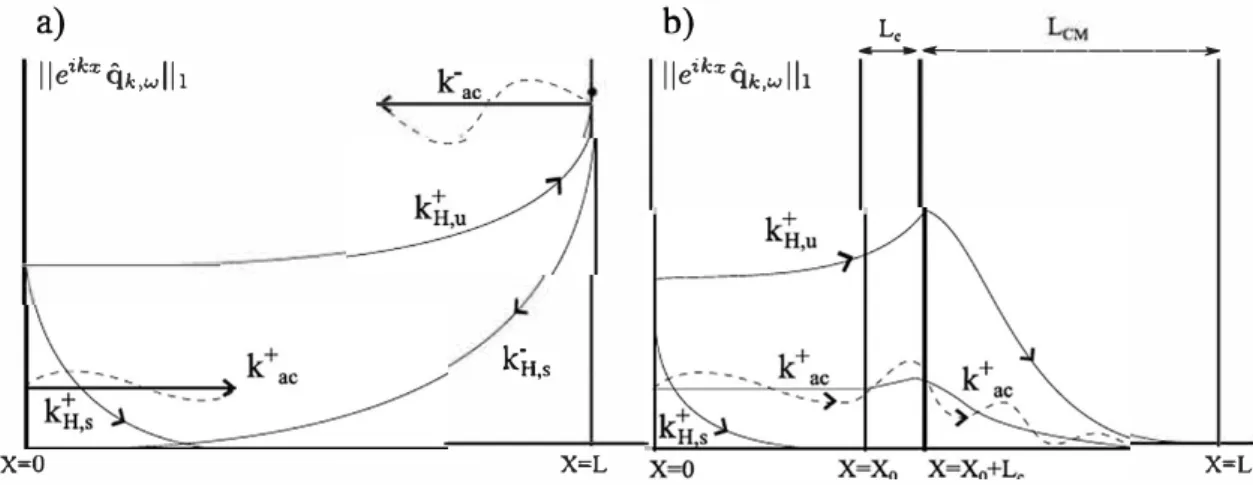
Fig. S. Sketch of the propagation of hydrodynamic and acouscic waves, where ror the sake of illustration

L™

and le are depiccect incencionally large wich respect co the physical domain. ln ordinace the amplitude or a plane-wave, Ue""'<Lc..,11,, is represenced. (a) wichouc CM : waves

,ç

_{_.,} and kt are presenc ac the outlet, chus leading co renecced waves (only the reneccions caused by wave k:.u are represenced). (b) wich CM, and choosing Yc according co (33): Waves k:,, and k! are damped when reaching the boundary, so no reneccion is generaced.

Here

kt

is the spatially unstable Kelvin-Helmholtz wave and

kt

is a

'"

spatially stable wave which does not lead to particular

priblems but has to be retained in the discussion. Note that bath

solutions belong to the

kt

category and should thus be present

in the solution of the problem for x � +oo. The zero-thickness

shear layer does not possess any

kïj

solutions (for reasons dis­

cussed in Huerre & Rossi (

16

1) but continuous

U(y)

profiles admit

such solutions which, except in cases where U

00

and/or

Uc

are

negative, are always located in the half-plane

lm(k)

< 0 and far

away from the

kt s

solutions.

,u

5.2.2. Effect of CM on plane-waves

For the present discussion we will thus restrict to five solu­

tions. Acoustic waves

ktë,

the KH waves

kt s

and a possible

kij

solution. The behavior of these solutions as

'"l

x

l

� oo is one of

the three following cases:

(i)

Dominant

if

lm(kx)

_{< 0, i.e.}

arg(kx) E

[-rr, 0)

(29)

(ii)

Evanescent

if

lm(kx)

> 0, i.e.

arg(kx) E

(0, rr]

(30)

(iii) Oscillating if lm(kx) = 0, i.e. arg(kx) = 0, 1r

(31)

We will consider the asymptotic effect of complex mapping equa­

tion

(

4

)

. The situation differs according to the argument of

w.

We

consider three cases:

Case 1: arg(w)

=

0

The case where

w

is real is particularly important as it is

relevant to bath the

Jorced problem

resolved in frequency do­

main, and to the

stability problem

at marginal conditions.

Fig. 6

(a)

sketches the location of the fwe considered plane-wave solutions

in the complex k-plane. The region

lm(k)

< 0 corresponding to

dominant solutions in the absence of mapping is indicated by the

gray area. Bath solutions kt

u

and kij

belong to this region, while

kt s

is evanescent and k!

are bath oscillating.

·

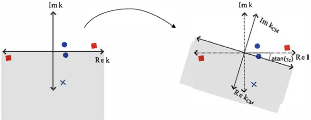
As sketched in

Fig.

6(

b

)

, the effect of the complex map­

ping Eq.

(4)

for xis

to 'tilt' the boundary between dominant and

evanescent solutions by an angle arg(y

c)-

As a result, the choice

Yc

> 0 is sufficient to turn the physically relevant

k;t;

into an

evanescent wave and the unwanted

k;;;

into a dominant wave,

which will thus be damped as it propagates backwards. However,

if Yc is small, the solution

will

still contain a dominant kt

u

wave.

This solution corresponds to the spatially growing

'

Kelvin­

Helmholtz instability, and is perfectly relevant from a physical

point of view. However, if the spatial growth of this wave is

larger than the spatial damping of the backward-propagating

k;;;

induced

by

the mapping, the

k;,

solution may still be present in

the domain as a reflection of the

kt u·

The remedy to avoid this is

to chose

Yc

such as

kt u

becomes evanescent, see

Fig. 5

(b).

This

requirement leads to the following condition:

+

.

IUoo - Ucl

arctan(yc) > - arg(k

H

,u), 1.e. Yc > ----

(32)

Uoo

+

Uc

The corresponding situation, where only the

k;,

wave is dom­

inant, is sketched in

Fig. 6

(b). CM is also effective in a situation

where

kt u

does not decay enough before reaching the outer

boundary,' but backward propagating wave does before escaping

complex mapping region and reaching the physical domain. lt

is found that in that case CM is more effective for compressible

flows and Eq.

(32)

turns to be the condition for the low Mach

limit, see

Appendix D

for details.

Imk Imk

•

•

_Rek

X

Fig. 6. Diagram displaying a complex mapping ç,(X) for a real rrequency w, such chat arg(w) = o, in the complex plane or the wave-veccor k. Red squares represenc spatial acouscic modes fç, whereas blue circles represenc hydrodynamic modes k;_, and the blue cross denoces the kjj mode.

•

Imk

•

_•

•

Rek

Imk

Fig. 7. Diagram displaying a complex mapping 9,,(X) ror an unscable rrequency w, in the complex plane or the wave-veccor k. Legend or symbols is the same as in Fig. 6. Imk

�

Imk

•

_•

•

Rek

X

Fig. 8. Diagram displaying a complex mapping 9,,(X) ror a stable rrequency w, in the complex plane or the wave-veccor k. Legend or symbols is the same as in Fig. 6.

Case 2: 0 < arg(w)

«

!}

This second case corresponds to the expected behavior of a

temporally unstable mode.

As

seen in

Fig. 7

, this case is more

favorable, as the

k;

wave is already in the dominant region

without need of the mapping. If one wants to turn the

kt

u

wave

into an evanescent as in

Fig

.

5

(b)

one needs to choose

Yc

'in such

a way it possesses a sufficient decay (see

Fig. 7

):

(IUoo -Ucl)

arctan(yc) > arctan

Uoo + Uc

-

a�(w)

Case 3:

-!}

«

arg(w) < 0

(33)

Now we consider a value w

corresponding to a stable global

mode. This case is the less favorable, as without mapping (see Fig. 8

(a)). The k�

wave is in the dominant region, meaning that it will

be amplified as propagating backwards, destroying any chances to

correctly compute the mode. The condition to change this mode

into a dominant one and turn the

kt

u

into an evanescent one

is still given by Eq.

(

33

)

, but it is more restrictive here than in

previous cases since

arg(w)

< O.

6. Application cases

6.1. Incompressible flow through a single hale

ln this section we will discuss the application of the complex

mapping methodology to incompressible Navier-Stokes equa­

tions. The hole diameter is considered as the reference length,

denoted by L,- and the characteristic scale, Ur is the mean velocity

across the hole. The application case is the flow past a single hole

of finite thickness. This configuration has been recently studied by

Fabre et al. see (

8

, Sec. 3) for the definition of the problem and a

discussion about boundary conditions. Severe numerical difficul­

ties arise in the solution of the linearized Navier-Stokes equations

,,,-r

----

Table 3

/�

, ,,,:""

;_ --1--- ---- ----·-- .

L_ --- --�· ---�-�--- �-�--�

-

-Fig. 9. Sketch or the now configuration representing the oscillating now past a circular hole in a thick plate.

Table 2

Description or meshes M; ror i

=

1, 2, 3. N0 denotes the number or verrices of the mesh. GeometricaJ parameter l"'' denotes the axial longitude of the mesh and Rour is the radial extension or the numerical domain.

Description of numerical domains M1 - M3

Mesh Lour Rour Xo Le Yc Nu

M1 20 15 5 0.5 17915

M2 30 20 30695

M3 60 20 78300

due to the strong spatial amplification of linear perturbations, in particular pressure (see Fig. 9).

An artificial boundary treatment is a mandatory technique for this type of study. Large amplifications of linear perturbations lead to physical perturbations far downstream the hole. ldeally, this would require an infinite domain, at least in the streamwise direction. However, numerical computations are realized in trun­ cated domains. If the computational domain is not sulficiently large, that is amplitude of the perturbed field is negligible close to the outer boundary, "spurious eigenvalues" constituting the discretized version of the continuous spectrum may arise. ln the case of large perturbations, these "spurious eigenvalues" can be even located in the unstable side of the spectrum and close to discrete physical eigenvalues as Reynolds number increases.

The linear stability study of the flow past a hole in a thick plate shows that dynamics of Re < 3000 can be explained by the presence of three discrete physical modes, here denoted by H1, H2 and H3. For validation purposes we have designed three computational meshes

M

i for

i

=

1, 2, 3, the first one with CM

uniquely in the axial direction and the other two without any ABC but with longer axial dimension, denoted Lout (see Table 2).

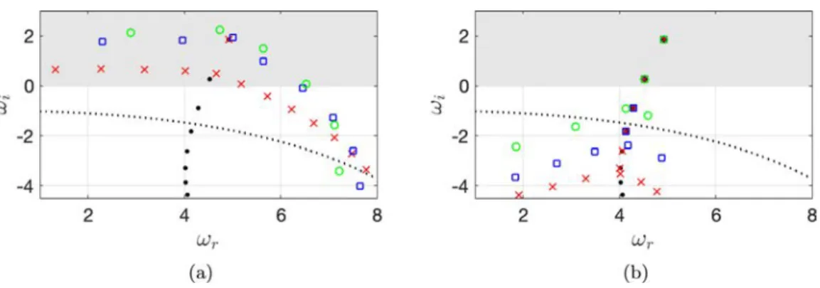
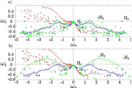
Fig. 11 displays the numerically computed spectra using nu­ merical domains M1, M2 and M3 for Re= 1700, Re= 2000. The

spectra here displayed presents three discrete eigenvalues Hi for

i

=

1, 2, 3 and a set of "spurious eigenvalues", named arc-branch by Lesshafft (6), which arise due to non-local feedback mecha­ nism of spurious pressure signais from the truncated boundary

4

x=Lm

LJ

2

0

-2

n

-4

_-2

₀

₂

₄

₆

₈

EigenvaJue computations ror Re= 1600.

M1 -0.1156i + 0.5024 0.0854i + 2.0985

M2 -0.1259i + 0.5017 0.13916i + 2.1051

M3 -0.1189i + 0.5017 0.0826i + 2.107

Table 4

EigenvaJue computations ror Re= 2000.

M1 -0.0435i + 0.5615 0.3032i + 2.2436 M2 -0.0421i + 0.5645 0.3114i + 2.2467 M3 -0.0420i + 0.5628 0.2965i + 2.2399 -0.0926i + 4.1230 -0.105 li+ 4.1359 -0.0944i + 4.1240 0.2418i + 4.3184 0.2287i + 4.3268 0.1232i + 4.2807

and upstream locations. Computations of the spectra without ABC, M2 and M3, lead to the presence of unstable spurious eigen­ values (w; > 0). Moreover, as the Reynolds number increases they tend to approach discrete eigenvalues H;. The use of CM results in a good separation of physical and spurious eigenvalues. However, CM methodology with Yc > 0 does not allow to identify the

complex conjugate modes of Hi located in w, < O. The exploration of the other side of the spectrum can be determined by choosing

Yc < O. ln Fig. 10 it is possible to visualize the elfect of complex

mapping on the structure of the pressure component of the H2

mode. lndeed, one may observe how CM can efficiently transform a convective dominant wave into evanescent, hence any non-local effect, i.e. arc-branch eigenvalues, is avoided.

Finally, Table 3 and Table 4 display a comparison of the nu­ merical elficiency of numerical methodologies M; for

i

=

1, 2, 3 for the computation of discrete eigenvalues. Following, similar arguments as in Fabre et al. (8) we conclude that CM methodology allows a precise identification of discrete spectrum with a lower number of vertices with respect to methodologies without ABC. 6.2. Hole-tone configuration

The problem of the flow passing through a circular hole in a plate is encountered in many practical applications and has been widely studied by experimental and numerical investigations. This situation is encountered in various applications, including the whistle of a tea kettle, which has been studied by Henrywood & Agarwal (17) or birdcalls (devices used by hunters to imitate bird singing) analyzed by Fabre et al. (18) (see Fig. 12).

Attempts to characterize the instability mechanism were pre­ viously made using incompressible (see Fabre et al. [181) and compressible (see Longobardi et al. (191) LNSE. These efforts allowed to identify the dilficulties associated to boundary condi­ tions. The diameter of the first hole is taken as the characteristic length scale L, and the mean velocity along the hole as the refer­ ence velocity scale U,. This test case has been previously used to

3600

83

0

-83

-3600

10

12 14

16

a)

Fig. 11. Specrrum compured wirh rhree meshes. x (red online) denores eigenvaJues compured wirh Mi. ,. (green online) with M2 and + (blue online) wirh M3 for (a)Re= 1700 and (b) Re= 2000. (For inrerprerarion of the references ro color in rhis figure legend, the reader is referred ro the web version of Chis article.)

1

10 Fig. 12. Sketch of the hole-rone configuration, frame of reference and definirion of geomerricat paramerers. An exampte of compurarionat mesh is also reporred in lighr gray. An acruat birdcall is depicred in the upper righr corner. e den ores

the thickness of the caviry wall, radius of hales Rh.i, i

=

1, 2, radius and tengrh

of the caviry are denored by Re •• and Hca, respecrivety. Values of geomerricat

paramerers can be round in Longordardi er al. Il 9 ].

show CM efficiency by Sierra et al. [20), where more details about governing equations, i.e. compressible Navier-Stokes, boundary conditions and methodology may be found.

6.2.1. Eigenvalue computations

We study some characteristics of the spectrum of the flow by solving Eq. (19) in the compressible setting. Linear dynamics of the birdcall flow at a sufficiently high Reynolds number is governed by a set of unstable discrete modes, the continuous spectrum remains stable. ln the studied range of

Re

and M00, we have appreciated the presence of four unstable modes up to

Re

=

1600. These modes have been computed with two techniques, sponge as boundary condition at the far field and complex mapping. Artificial boundary conditions are needed to compute physically relevant modes and to avoid the appearance of spurious modes in the spectrum due to boundary conditions.

To identify these modes at threshold we have used complex mapping. Complex mapping technique allows to tilt the continu­ ous branch of the spectrum to leave discrete modes isolated and easy to be identified at the threshold. This phenomenon is briefly described in Section 4. At Fig. 13, spectrum is displayed for two Reynolds numbers at M00

=

0.05. The spectrum corresponding

to the simulation with sponge boundary condition at far field at threshold presents some discrete eigenvalues and a continuous branch along the real axis. Let us consider the case

Re

=

320 and M00

=

0.05. At that configuration Mode 1 is neutrally

stable. However, we are not able to identify it by numerical means since it is clustered inside the continuous branch. So, one should increase further the Reynolds number hoping to find the

mode in the unstable zone. With the complex mapping technique continuous branches are rotated from the origin with an angle arg x whereas discrete modes remain invariant. This allows to identify modes near and at threshold. These modes are displayed in Fig. 14. ln that figure it is possible to appreciate the hydro­ dynamic instability which is the part of the mode of highest amplitude. lt is possible to remark a few properties of these modes. The pressure is fairly constant in the cavity but it is not constant as it has been reported by Longobardi et al. (19). The spatial structure of pressure mode inside and outside the cavity is proportionally dependent of the temporal frequency w, which indicates a direct link between the quantization of frequency and pressure oscillations between bath hales (see Fig. 14 (a) and (b) for the structure of Mode 1 and 2 at

Re

=

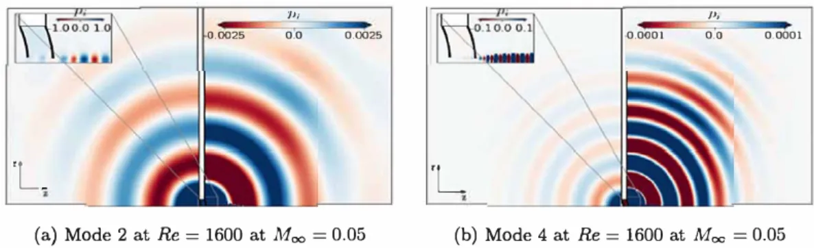
1600 and Fig. 16 (b) for the frequency). Similarly, as w increases a given mode tends to have its support farther from the cavity. From the vorticity field of Fig. 14 it is possible to observe the antisymmetric pattern of vorticity inside the cavity for mode 1 and mode 2 and the tendency of the shear layer to become symmetric and reduce its thickness as w increases, this is specially remarkable for mode 4. Finally in Fig. 15, we depict the imaginary part of the pressure of global modes for

Re

= 1600 and Moo = 0.05 for Mode 2 and Mode 4. lt is possible to observe the radiation of acoustic waves propagating into the far field as spherical waves. Acoustic radiation between Mode 2 and Mode 4 differs in wavelength Àac and acoustic directivity. Wavelength decreases as w increases whereas the acoustic directivity seems to change when the acous­ tic wave is able to penetrate into the cavity as it has been previously observed by Longobardi et al. [19).

For this study we have used four meshes which are shown in Table 5. M1 has been used as a reference test case computed with sponge layers. Remaining meshes are used with CM method­ ology which allows to greatly reduce the size of the domain and the number of points. The size of the domain is denoted by [Xmin,Xmwc, Rmwcl, where Xmin is the x-coordinate of the inlet, Xmwc is the x-coordinate of the outlet and Rmwc corresponds to the outer radius of the domain. Please note that the minimum size of the sponge section, denoted by lXmin,Xmwc, Rmwcl in Table 5, is the minimum domain size to elfectively damp acoustic waves. The outer boundary is located at a distance approximately three times the acoustic wavelength of the first bifurcated mode. The reduction in computational time from the use of Sponge or Com­ plex mapping can be also perfectly visualized in Table 5 where it

'

_'

0.5

1!11 19

3

0

)O(X*'°'

3

-0.5

0 _xx

-10

-5

0

5

10

Wr

(a) Spectrum at

Re=

640

M

oo

=

0.05.

0.5

0

-0.5

...

�

'!SI

.tl.

�liÏICg D

_�

a

¾

,

-�lt<' CnP

I

�

0 of O ,s5b� X c:POO X Ill O X

�X

181

'

i

o

_�

_,

""î

_�

�

dl) X

�

�

�

i!ilo c§l Clèx 'tPo

-10

-5

0

5

Wr

10

(b) Spectrum at

Re

=

320

M

oo

=

0.05

Fig. 13. Specrrum near cwo bifurcation Re at M00

=

0.05. Legend : o are used ta denore eigenvalues carresponding ta CM. Red is used for Yc

=

0.1 and blue for Yc = 0.15. Black x denores those eigenvaJues compured wirhour artificial boundary conditions. (For incerpreration or the rererences ta color in this figure Jegend, the reader is rererred ta the web version of this article.)

(a) Mode 1 at Re= 1600 (b) Mode 2 at

Re= 1600

-1.4 -0.5 1.4

..

_.._'À-.. , ... -

--27.;i20.8 27.2

(c) Mode 3 at

Re=

1600 (d) Mode 4 at Re= 1600

Fig. 14. Ir displays the four unstable modes at Re

=

1600 and M00

=

0.05. Toe real part or the pressure mode Pn and the imaginary part of the vorticicy !1; are

shown for each mode at the upper and Jower si des of each figure respectively.

is displayed the time needed to compute the leading eigenvalue with each of the considered meshes.

Computations with mesh M1 were carried out in serial with

an Intel i7 2.6 GHz whereas numerical tests for M; for i = 2, 3, 4 were computed with an Intel i7 2.2 GHz. Computational time takes into account the computation of the baseflow and the

leading eigenvalue at Re

=

400 and M00

=

0.05. The gain in

computational rime between Sponge and CM is around 50 for the finest mesh and 125 for the coarsest. This gain in performance is due to the fact that the domain size of the mesh is greatly

reduced, therefore reducing the number of elements required for the computation.

Concerning precision, a comparison between the four consid­ ered meshes is displayed in Fig. 16. ln that figure it is possible to observe in (b) linear frequency results are in agreement between the two considered methodologies. Whereas for the linear growth despite the fact the good fit between both methodologies and the four considered meshes there is a slighter disagreement between M4 and M1 for the mode with linear frequency around w, � 9 at high Re. The difference in the growth rate between M3 and M1 is

1>;

0.0025 0.0 0.0025

'

L

_

(a) Mode 2 at

Re=

1600 at

M00

=

0.05

0.0001

'L

f);

0.0 0.0001

(b) Mode 4 at

Re=

1600 at

M00

=

0.05

Fig. 15. lmaginary part or the pressure p; or cwo direct modes the second mode ac the Jeft and the rourch mode ac the righc. The main figure displays the radiation or the acouscic field whereas the zoomed region shows the spatially Jocalized hydrodynamic mode.

1 0.8 0.6

3

_0.4

,:,.

...

.,:,".t .:J, ..

�

0.2

�·

$

-

{

!

0 400 800 1200 1600 Re

(a) Linear growth rate

w,

evolution of the

four unstable branches as a function of

Re.

10 - Sponge _{•••• 1} 9 -CM-M2

""""'"'

î

-CM-Ms 8 -CM-M4 ,._.,, ....... Ai,, 7

:t

₆

,

.

.

...

.

....

..

.

5

.,,.

..

_,,.

..

_�

�·---·

..

4 3 400 800 1200 1600 Re

(b) Linear frequency

Wr

evolution of the

four unstable branches as a fonction of

Re

Fig. 16. Comparison or CM wich sponge ror the four unscable branches. Black lines are used co denoce the resuJcs compuced wich the sponge mechod, whereas gray, blue and red are used ror the mesh generaced wich the mesh adaptation algorichm detailed in the review article or Fabre et al. (9). Solid lines denoce the lirsc mode, Joosely dashed lines the second, dash dotced the third and densely dotced the rourch one. (For incerpreracion or the rererences co color in this ligure Jegend, the reader is rererred co the web version or this article.)

Tables

Mesh definition and performances. IXmin, XmCDC, R....,.] denoces the size or the compucacional domain, Xo the location above which the

CM is applied (in both (r, x) directions) and N, the number or mesh vertices where the boundary conditions are erreccively applied. The table also displays the compuced eigenvalue w and the cime required for computation Re= 400 and M00

=

0.05. The required

cime co perform a computation or ba.senow and Jeading eigenvalue wich a single processor is displayed.

Mesh Methodology N, [Xm;,, XmCDC, R....,.] Xo Yc w Time (s)

Sponge CM CM CM 1211054 31986 40942 14337 (-120, 120,130] (-30,30,30] (-80,80,80] (-30,30,30]

lower than 5 % in the worst case scenario, which corresponds to

the growth rate of Mode 4. ln this case the relative error is large

because of the small magnitude of the growth rate.

6.3. Flow past an airfoil

Low Reynolds number flow past an airfoil is a flow con­

figuration which has attracted interest from micro-air vehicles

or bio inspired air vehicles designers. Airfoils in these types of

configurations are usually configured to operate at high angles

of attack . Characteristic length and velocity scales are the chord

length of the airfoil profile and the far field uniform velocity. Flow

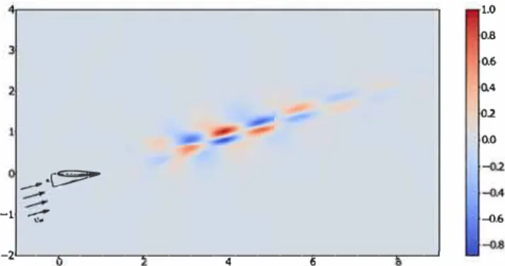
unsteadiness is encountered in the separated shear layer due to

a Kelvin-Helmholtz instability and in the wake of the airfoil in

the form of a Von Karman vortex street. ln the past Zhang &

Samtaney (

21

] (

22

] have carried out the study of a NACA 0012

profile at angle of attack

a

=

16

°

_{. ln the current section we}

10 40 10 0.2 0.2 0.15 4.7574 + 0.0792i 4.6922 + 0.0666i 4.7151 +0.0945i 4.7051 + 0.0747i 83944 s 1655 s 1421 s 669 s

reproduce previous results of the NACA 0012 airfoil for a given

flow configuration. Effectiveness of the CM methodology will be

shown by a parametric study of the length of the CM layer and

cross comparison with reference results.

ln

Table 6

, it is displayed the leading eigenvalue for several

meshes M

1 -

M.t which correspond to different lengths of CM

layer . CM is activated outside a rectangle whose upper right

corner is [X

0,

Y

0]

and its lower left corner is [-Xo, -Y

0]

with CM

parameters

Yc

=

0.3 and

Le

=

5.

Rout

is the radial extension of

the numerical domain and

LCM � Rout

- 10. Acoustic wavelength,

Àac

=:;

(d--+1},forMoo

=

0.1

atRe

=

lOO0is aroundÀac

�

28,

where length is non-dimensionless with respect to the chord of

the airfoil. A length of the CM region, of around � � [5 0, 6 0] is

sufficient to capture the leading eigenvalue, which has been also

computed with sponge layers, see M

5.

Nevertheless, M

1

whose

length of the complex mapping region is

LCM �

1'

presents