Development and Identification of a
Closed-Loop Model of the Cardiovascular
System Including the Atria ?
Antoine Pironet∗ James A. Revie∗∗ Sabine Paeme∗ Pierre C. Dauby∗ J. Geoffrey Chase∗∗ Thomas Desaive∗ ∗Cardiovascular Research Center, University of Li`ege, Li`ege, Belgium
(e-mail: a.pironet@ulg.ac.be).
∗∗Department of Mechanical Engineering, University of Canterbury, Christchurch, New Zealand.
Abstract: The atria play an important role in cardiac function. The introduction of two chambers representing the atria in an existing model of the cardiovascular system could provide useful information.
A previously validated cardiovascular system model is modified to include the atria, whose behaviour is modelled in an original way. An a wave pressure independent of the volume is introduced to make the model more realistic. This is one of the ten new parameters that are introduced in the atrial model. Six of these parameters are identified with an extension of the previously existing parameter identification method. A method to infer important atrial pressure characteristics from the ventricular pressure waveform is also developed.
Identification of the model parameters with and without atria are performed using data sets from a pulmonary embolism pig trial. The error is bigger in the model containing the atria, but remains of the order of measurement errors. The model with atria provides useful information about these two new compartments, without requiring the need for new measurements. This work is a useful improvement of the already existing model and identification methods as it now allows characterization of atrial function.
Keywords:Mathematical model, lumped-parameter system, parameter estimation, physiological model.
1. BACKGROUND
Cardiovascular diseases are the highest cause of mortality in Europe (Statistics Explained (2011)) and in the USA (Xu et al. (2010)). They are also a major cause of ad-missions in intensive care units (ICU). Even with a proper amount of data, patients in ICU are difficult to treat, this is in part due to the fact that a diagnostic is hard to establish because of the limited amount of measurements available. In addition, these measurements are mainly external (e.g. central venous pressure, arterial pressure, electrocardio-gram...) and thus do not provide any accurate information on the internal functioning of the heart, as, for example, the flow in the heart valves. Yet, this kind of information is of extreme interest in the study of many diseases, such as valvular dysfunctions.
A mathematical model of the heart can yield a clear physi-ological picture from data hard to understand at first. Such a model should be usable at bedside and, consequently, should only require commonly available measurements. Second, it should provide a reasonably correct picture of the intrinsic hemodynamic, which cannot be seen on the ICU monitors. Finally, the model has to be robust, in order
? This work was financially supported by the French Community of
Belgium (Actions de Recherches Concert´ees - Acad´emie
Wallonie-Europe).
to give correct predictions for all patients and conditions, and fast, to predict changes in real-time.
Simple lumped models will be prefered to more detailed finite-elements approaches. Such models do not perfectly reproduce the reality but focus more on the macro-physiological trends. Thanks to their simplicity, the in-volved equations can be solved in a few minutes on a classic computer.
The starting point of this work is the model developed by Smith (2004). It represents the cardiovascular system (CVS) in a very simple way, with six elastic chambers linked by vessels, modelled as flow resistances. This model, even if simple, takes into account complex effects such as ventricular interaction and valve dynamics (Smith et al. (2004)). The equations of this model are ordinary differen-tial equations involving 32 parameters whose values are at first unknown but have to be identified so that the model can be used. Two parameter identification methods have been developed and applied to the model of Smith et al. (Hann et al. (2006); Starfinger (2008)).
The atria play an important mechanical role in the cardiac function. They initiate the cardiac contraction by maxi-mally filling the ventricles before blood ejection. Patholo-gies involving atria are numerous (fibrillation, excessive dilation, etc.) and are often linked to valvular pathologies.
The goal of the present work is to insert into the model of Smith et al. two chambers representing the atria. This will make the model more realistic from a physiological point of view and will provide atrium-related information that could help to detect atrial pathologies more easily.
2. METHODS 2.1 Original CVS Model
The model used to represent the CVS has been developed by Smith (2004). It is a lumped model consisting of six elastic chambers, representing the left (lv ) and right (rv ) ventricles, the aorta (ao), the vena cava (vc), the pul-monary artery (pa) and the pulpul-monary vein (pu). The six chambers are linked by vessels having a given flow resis-tance. Those vessels are, respectively, the systemic (sys) and pulmonary (pul ) circulations and the mitral (mt), aortic (ao), tricuspid (tc) and pulmonary (pv ) valves. In addition to a flow resistance, the valvular behaviour is modelled with elements analogous to ideal diodes. For simplicity, inertia of the blood is not taken into account in this model, as the corresponding parameters do not play an important role and are difficult to identify. The model also takes into account the septal motion during cardiac contraction, following a formalism developed by Chung (1996).
The model chambers are characterized by two variables: their volume (V ) and the pressure (P ) inside of the cham-ber. The two elastic chambers representing the ventricles are said to be active, which means that the relationship between the pressure and the volume is variable. More pre-cisely, it varies between the end-systolic pressure-volume relationship (ESPVR) and the end-diastolic pressure-volume relationship (EDPVR), namely:
ESPVR: Piv(t) = Eiv(Viv(t) − Vd,iv) (1) EDPVR: Piv(t) = P0,iv(eλiv(Viv(t)−V0,iv)− 1) (2) where Eiv is the end-systolic elastance, Vd,iv, the end-systolic volume at zero pressure, V0,iv, the end-diastolic volume at zero pressure and P0,iv and λiv are parameters of the nonlinear relationship (2). (For the rest of this study, index i has to be considered as l (left) or r (right).) Transition between those two extreme relationships is weighted by an activation function, varying between 0 and 1 and denoted eiv(t). Consequently, the pressure in a ventricle at any moment t of the cardiac cycle is linked to the volume by:
Piv(t) = eiv(t)Eiv(Viv(t) − Vd,iv)
+(1 − eiv(t))P0,iv(eλiv(Viv(t)−V0,iv)− 1). (3) The other elastic chambers are passive, which means that their volume and pressure are linked by a constant, the elastance Ej.
Pj(t) = EjVj(t), with j = vc, pa, pu or ao. (4) The volume variation in the six elastic chambers can be derived from the continuity equation:
˙
V(t) = Qin(t) − Qout(t) (5)
where Qinand Qoutare flow coming in and going out of the chamber. Equation (5) does not take into account the heart valves, whose role is to regulate blood flow. More precisely, their role is to close to prevent backwards flow. Hence, to correctly model the effect of the valves, a negative flow has to be replaced by a zero flow. Mathematically, it can be easily done by replacing each flow Q(t) controlled by a valve by H(Q(t))Q(t), where H denotes the Heaviside function.
Each pair of elastic compartments of the model is linked by a vessel. Each of these vessels is characterised by an hydraulic resistance, denoted R. The relationship between flow, pressure and resistance is given by Poiseuille’s law:
Qk(t) =
Pu(t) − Pd(t) Rk
, k= sys, pul, mt, ao, tc or pv (6) where Pu(t) and Pd(t) represent the pressure up and downstream of the vessel.
2.2 Introduction of the atria in the model
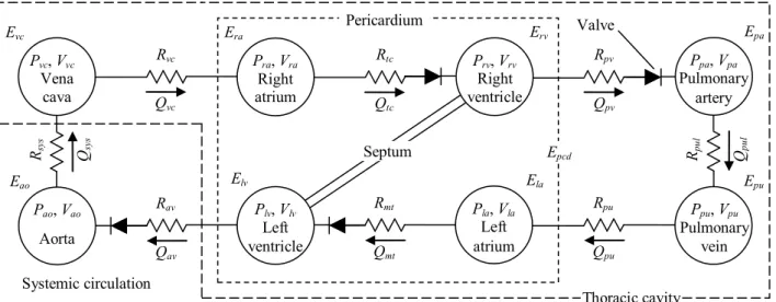
Two new elastic chambers representing the atria are added to the initial 6-chamber model. The corresponding 8-chamber model is shown in Figure 1. Two new resistances have been added between the venous chambers and the atria. On the left side, the new resistance is the pulmonary vein resistance Rpu and on the right side, the vena cava resistance Rvc.
Since the atria are also active chambers, as for the ventri-cles, the relationship between their pressure and volume is not constant. An original model has been developed to describe the atrial behavior. During atrial filling, blood flows into the atria, consequently increasing pressure and volume in these chambers. A passive pressure-volume (P-V) relation, namely
P(t) = EV (t) (7)
is thus well suited to describe this part of the cardiac cycle. However, during atrial contraction, volume decreases while pressure simultaneously increases. These two variables can thus not be linked by (7) anymore. One solution, as done by Lau et al. (1979), is to add a time-dependent elastance E(t) and a dead volume V0(t) in (7). This gives:
P(t) = E(t)(V (t) − V0(t)). (8) During atrial contraction, the dead volume decreases, as does the atrial volume. These two variations compensate each other and the shape of the pressure curve is described by the time-varying elastance.
The inconvenient of this approach is that it significantly increases the amount of parameters needed to describe the two curves E(t) and V0(t). We thus have chosen a different but similar approach, describing pressure in the atria by the following equation:
Pia(t) = eia(t)Pia,act+ (1 − eia(t))EiaVia(t), (9) where eia(t) is the atrial driver function, equal to 1 during atrial contraction and to 0 during filling. The two constant parameters Pia,actand Eiarespectively describe the pressure developed during atrial contraction and the elastance during filling.
P, V Pulmonary Artery P, V Right Ventricle P, V Left Ventricle P, V Aorta P, V Pulmonary vein P, V Vena Cava Eao Ees,lv f Evc Ees,rvf Epa Epu Rav Rmt Rsys Rtc Rpv Rpul Septum Qav Qmt Qpul Qsys Qtc Qpv Pericardium Lav Ltc L pv Lmt Thoracic Cavity Pra, Vra Right atrium Era Erv Rtc Rpv Qpv Qtc Ppa, Vpa Pulmonary artery Epa Rpul Qpul Ppu, Vpu Pulmonary vein Epu Elv Rmt Qmt Pao, Vao Aorta Eao Rav Qav Rsy s Qsy s Systemic circulation Epcd Valve Plv, Vlv Ventricule gauche Rmt Qmt Pao, Vao Artère aorte Rav Qav Rsys Qsys Ppu Pvc Ees,lvf Eao Prv, Vrv Ventricule droit Rtc Qtc Ppa, Vpa Artère pul. Rpv Qpv Rpul Qpul Pvc Ppu Ees,rv f Epa (a) (b) Thoracic cavity Pvc, Vvc Vena cava Rvc Qvc Evc Pla, Vla Left atrium Ela Rpu Qpu Septum Plv, Vlv Left ventricle Prv, Vrv Right ventricle Pericardium
Fig. 1. CVS model including the atria
As previously done in other studies, the atrial driver function is a gaussian function:
eia(t) = exp (−Bi(t − ∆ti)2), i = l or r, (10) where Bi describes the width of the driver function and ∆ti is a time shift indicating when the a wave occurs. Introduction of the atria in the model adds ten new parameters in the CVS model: Ela, Pla,act, Bl, ∆tl, Rpu, and their homologous for the right side. Identification of these parameters can be done by extending the initial identification method of Revie et al. (2011b) as explained in the following section.
2.3 Parameter Identification
A method aiming to identify the parameters of the CVS model described in the previous section has been developed by Revie et al. (2011b). This method has two important features. First, it is based on a simple proportional gain controller used to update the values of the parameters. Second, the identification is not performed directly on the 8-chamber model but on two smaller, simpler models whose parameters are identified before insertion in the complete model.
To identify a parameter, one has to find a direct or inverse proportional relationship between this parameter and an output variable of the model. It is obvious that such a relationship must be physiological. The ratio between the model output and the experimental measurement is used in an iterative process to obtain a better approximation of the parameter at each iteration. The parameter update is performed using one of the following equations:
• for a proportional relationship between parameter and model output:
paramnew= measurement model outputparam
old; (11)
• for an inversely proportional relationship between parameter and model output:
paramnew= model output measurementparam
old. (12)
The parameters identified by this method are shown in Table 1.
Table 1. Initial Parameter Values
Parameter Initial Value Units
Pvc 5 mmHg Ppu 5 mmHg Elv 2 mmHg/ml Erv 0.8 mmHg/ml Eao 2.5 mmHg/ml Epa 2.1 mmHg/ml Epu 0.01 mmHg/ml Evc 0.01 mmHg/ml Rmt 0.05 mmHg·s/ml Rav 0.04 mmHg·s/ml Rsys 2.5 mmHg·s/ml Rtc 0.04 mmHg·s/ml Rpv 0.03 mmHg·s/ml Rpul 0.4 mmHg·s/ml Rvc 0.105 mmHg·s/ml Rpu 0.16 mmHg·s/ml
Step 0: Direct Identification of Parameters from Data Before starting the identification process, some parameters have to be estimated from available data, as they are needed for the rest of the process. These parameters are the ventricular activation functions, and atrial parameters ∆ti and Pia,act.
The identification of the left ventricle activation function elv(t) is based on a method developed by Stevenson et al. (2010). This method uses the aortic pressure waveform and some of its characteristic points (extrema and inflexion points, among others) and links them to other character-istic points of the activation function. The same method is used to get the right ventricle activation function from the pulmonary artery pressure waveform.
Parameters ∆tiand Pia,actcan be directly identified using features of the available ventricular pressure waves. Let us denote the beginning and end of the diastole by tBD,i and tED,i. Parameter Pla,act is identified as follows:
Pla,act= max tBD,l≤t≤tED,l
where ∆Pav,l is a correction factor accounting for the mean pressure difference between left atrium and ventricle (4 mmHg for the left side). Equation (13) just says that the left atrial a wave pressure is estimated as the maximum ventricular pressure during diastole, plus a constant offset. The same procedure is done for the right atrial parameter Pra,act (with ∆Pav,r= 1 mmHg).
Parameters ∆tiare estimated as the times at which these maximal pressures occur:
∆ti= arg max tBD,i≤t≤tED,i
Piv(t). (14)
Step 1.1: Identification of the Systemic Model The two simpler models of the systemic and pulmonary circulations are obtained by setting constant pressure values in the ve-nous chambers. If ventricular interaction and pericardium pressure are supposed to be negligible, the left and right sides of the CVS model can be separated (Revie et al. (2011b)).
The systemic model comprises the left atrium and ventricle and the aorta. The first step of the identification process is to compute systemic (Rsys) and mitral valve (Rmt) resis-tances and aortic elastance (Eao). The measurements used to identify these parameters are the stroke volume and the amplitude and mean of the aortic pressure, respectively. Once all the previous parameters have converged, a second set of systemic parameters is computed. It comprises the pulmonary vein (Rpu) and aortic valve (Rav) resistances and the (constant) pulmonary vein pressure (Ppu). The pulmonary vein resistance Rpu is identified using the ratio of measured and simulated amplitude of the atrial v wave and the aortic valve resistance Rav is identified with the maximal aortic pressure gradient. (Since no atrial measurement is available, atrial v wave pressure is estimated as ventricular pressure at begin of diastole, plus the correction term ∆Pav,l.)
Pulmonary vein pressure Ppu is computed using mean atrial pressure and a correlation computed from data published by Chaliki et al. (2002):
Ppu= 0.92 ¯Pla+ 4.72, (15) where ¯Pladenotes mean atrial pressure. (Both Ppuand ¯Pla are expressed in mmHg.)
After update of the parameters Rpu, Rav and Ppu, the three previous parameters are re-identified. This process continues until a sufficient concordance with measured data is reached (relative errors less than 1 %).
Step 1.2: Identification of the Pulmonary Model The identification process for the pulmonary model is the same as for the previous one. First, pulmonary (Rpul) and tricuspid valve (Rtc) resistances and pulmonary artery elastance (Epa) are identified with the measured stroke volume and amplitude and mean of the pulmonary artery pressure. Then, three other parameters (vena cava (Rvc) and pulmonary valve (Rpv) resistance and (constant) vena cava pressure (Pvc)) are updated and the iterative process continues. The correlation used to identify vena cava pressure from mean right atrial pressure ¯Pra is a scaled version of (15):
Pvc= 0.61 ¯Pra+ 2.88 (16)
where pressures are expressed in mmHg.
Step 1.3: Identification of Ventricular Elastances When the two simple models are identified, ventricular elastances Elv and Erv are identified using a method conceived by Revie et al. (2011b).
Step 1.4: Computation of Ventricular Interaction and Pericardium Pressure At this stage, ventricular interac-tion and pericardium pressure are inserted in the model. These are computed using equations described by Starfin-ger (2008).
Step 2: Averaging of Valve Resistances Valve resistances (Rmt, Rav, Rtc, Rpv) are very sensitive to variations in measured data. However, from a physiological point of view, they remain constant between successive cycles. To ensure that valve resistances remain constant, steps 1.1 to 1.4 are repeated for each data set and valve resistances identified for each data set are averaged and kept constant for the rest of the procedure.
Step 3: Second Loop Once valve resistances are esti-mated, steps 1.1 to 1.4 are repeated, keeping valve resis-tances constant. Hence, corresponding measurements are not needed anymore. Stroke volume is used to identify venous resistances Rpu and Rpv so that estimation of v wave pressure from ventricular pressure is not needed during the rest of the identification procedure.
Step 4: Identification of Venous Elastances Once all the previous parameters have been identified, the two simple models are put back together and the two remaining parameters (the venous elastances, Epu and Evc) have to be computed. However, there is no reference measurement available to identify these parameters. We thus rely on the constant venous pressures Ppu and Pvc identified in the simple models and identify parameters Epu and Evc so that average venous pressures match constant venous pressures coming from the simple models. To do so, we use a numerical minimum finding routine.
2.4 Porcine experiments and data
The previously described identification method is applied to a trial of pulmonary embolism carried out on a pig under the control of the Ethics Committee of the Medical Faculty of the University of Li`ege.
The aortic pressure, the artery pressure and pressure and volumes in both ventricles were recorded every 30 minutes during 270 minutes, which yields ten different data sets for identification.
3. RESULTS
Simulations of the 8-chamber model gives pressure and volume curves for the atria that are consistent with exper-imentally measured curves. In particular, the atrial pres-sure wave presents the two characteristic a and c waves, resulting from the active emptying and passive filling of the atrium, respectively.
In this section, the outputs of the two CVS models (with and without the atria) are compared to experimental
0 0.1 0.2 0.3 0.4 0.5 0.6 65 70 75 80 85 90 95 100 105 110 Time (s) Aortic pressure (mmHg) Measurement Simulation (atria) Simulation
Student Version of MATLAB
0 0.1 0.2 0.3 0.4 0.5 0.6 0 20 40 60 80 100 120 Time (s)
Left ventricular pressure (mmHg)
Measurement Simulation (atria) Simulation
Student Version of MATLAB
0 0.1 0.2 0.3 0.4 0.5 0.6 55 60 65 70 75 80 85 90 Time (s)
Left ventricular volume (ml)
Measurement Simulation (atria) Simulation
Student Version of MATLAB
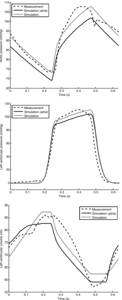
Fig. 2. Identification results for data measured 30 minutes after the beginning of the experiment.
measurements in order to verify the results and observe the influence of adding the atria to the model.
First, model outputs are compared with measurements used in the identification method in order to check that the models converged correctly. As an example, for measure-ments taken 30 minutes after the beginning of the experi-ment, simulated and reference aortic pressures are shown in Figure 2 (top). The agreement between experiment and simulations (of the models with and without atria) is very good. This is expected, since many of the characteristics of this curve are used in the identification process (the amplitude, the mean, the maximal slope and the general shape for approximation of the driver function).
Afterwards, the outputs of the two models are compared to measurements that were not used to identify model parameters, for example pressures and volumes in the ventricles. (To be precise, ventricular measurements are used to identify auricular parameters but not ventricular parameters.) Figure 2 (middle and bottom) shows that model outputs correctly predict ventricular pressures and volumes, which were not used in the identification process.
30 60 90 120 150 180 210 240 270 0.4 0.5 0.6 0.7 0.8 0.9 1 Time (minutes) Pulmonary resistance (mmHg s/ml) Simulation (atria) Simulation
Fig. 3. Evolution of the pulmonary resistance during pulmonary embolism. 30 60 90 120 150 180 210 240 270 1 2 3 4 5 6 7 8 Time (minutes)
Mean atrial pressure (mmHg)
Right atr ium Left atr ium
Fig. 4. Evolution of mean atrial pressures during pul-monary embolism.
In both models, the largest errors relate to the stroke volume. This comes form the fact that reference stroke volume is an averaged stroke volume for left and right ventricles (Revie et al. (2011b)).
Our parameter identification also allows to observe the influence of a pulmonary embolism on identified parame-ters. For example, as can be seen on Figure 3, pulmonary resistance increases during development of the embolism, as the pulmonary circulation gets obstructed. With the introduction of the atria in the model, the evolution of the mean atrial pressures can also be tracked during the embolism. As shown in Figure 4, both left and right atrial pressures can be seen to increase during the experiment. Table 2 summarizes the medians and 90th percentiles of relative errors for identification carried on the 10 exper-imental data sets. Relative errors are small (less than 0.5 %) for ¯Pao and ¯Ppa, since these model outputs were forced to match measured data during the identification. Errors on the other mean variables are more important and mainly come from differences in the stroke volume of the systemic and pulmonary compartments that the identification method does not take into account, as the reference stroke volume is the same for both ventricles (Revie et al. (2011a)).
From Table 2, it can be seen that adding the atria in the model does not cause an important increase of the errors. This validation step used a comparison with measurements that were not used during identification and shows that errors of the method are comparable to measurement errors (approximately 10 %). The interest of
Table 2. Median and 90th percentile of rela-tive errors (in %) between measured data and
model outputs with and without atria.
Output Error No atria Atria
Mean aortic Median 0.1 0.4
pressure 90th percentile 0.2 4.2
Mean pulmonary Median 0.1 0.5
artery pressure 90th percentile 0.3 4.9
Mean left Median 1.5 2.6
ventricular volume 90th percentile 3.7 4.2
Mean right Median 1.5 1.7
ventricular volume 90th percentile 3.8 5.0
Mean left Median 5.3 5.2
ventricular pressure 90th percentile 11.4 12.2
Mean right Median 3.9 3.1
ventricular pressure 90th percentile 8.5 9.0
the method developed in this work is significant, since it gives supplementary information (about the atria) without introducing the need for new measurements.
4. DISCUSSION
The use of lumped-parameter models have known limita-tions due to their simplistic nature. For example, as can be seen in Figure 2 (top), the dicrotic notch of the aortic pressure wave is not represented. This notch is caused by complex wave interactions that cannot be taken into account in such a simple model. In our case, the use of a lumped-parameter model is fundamental since we are dealing with parameter identification, which require many model simulations. Furthermore, as the final goal is to obtain a real-time monitoring tool, these simulations have to be very fast, which is only feasible with small models. The new model used for the characterization of the atria is load-dependent, since for any loading volume in the atria, the active pressure will be the same. This could cause too much ejected volume in case of small loading volumes of the atria. This choice of a load-dependent model was made for the sake of the number of parameters. Indeed, another way to correctly account for atrial behavior is to use the pressure-volume equation (8) introduced by Lau et al. (1979), but this would significantly increase the amount of parameters.
Of course, some points of the identification method devel-oped here have to be examined more deeply or even im-proved. For instance, it is important to check the validity of the hypotheses formulated to deduce features of the atrial pressure waveform (a wave timing and amplitude and v wave amplitude) from the ventricular pressure waveform. It would thus be highly interesting to test this method on an experimental data set including atrial measurements to quantify the errors.
5. CONCLUSIONS
This paper shows how a six-chamber model of the car-diovascular system and the corresponding identification method have been modified to include the atria. The goal was to identify a maximal number of atrial parameters on basis of a minimal amount of supplementary data. The method that is developed in this paper fully achieves this goal, since the identification of the atrial parameters
is done without requiring new measurements. Hence, this work gives a new model of the cardiovascular system in-cluding the atria and the parameter identification method needed to make it patient-specific. It provides a first step towards real-time monitoring of valvular pathologies for which precise characterisation of atrial function is of great importance.
REFERENCES
Chaliki, H., Hurrell, D., Nishimura, R., Reinke, R., and Appleton, C. (2002). Pulmonary venous pressure: re-lationship to pulmonary artery, pulmonary wedge, and left atrial pressure in normal, lightly sedated dogs. Catheterization and cardiovascular interventions, 56(3), 432–438.
Chung, D. (1996). Ventricular interaction in a closed-loop model of the canine circulation. Master’s thesis, Dept. of Electrical and Computer Engineering, Rice University. Hann, C., Chase, J., and Shaw, G. (2006). Integral-based
identification of patient specific parameters for a mini-mal cardiac model. Computer methods and programs in biomedicine, 81(2), 181–192.
Lau, V., Sagawa, K., and Suga, H. (1979). Instantaneous pressure-volume relationship of right atrium during iso-volumic contraction in canine heart. American Journal of Physiology-Heart and Circulatory Physiology, 236(5), H672–H679.
Revie, J., Stevenson, D., Chase, J., Hann, C., Lamber-mont, B., Ghuysen, A., Kolh, P., MoriLamber-mont, P., Shaw, G., and Desaive, T. (2011a). Clinical detection and mon-itoring of acute pulmonary embolism: proof of concept of a computer-based method. Annals of Intensive Care, 1(1), 33.
Revie, J., Stevenson, D., Chase, J., Hann, C., Lamber-mont, B., Ghuysen, A., Kolh, P., Shaw, G., Heldmann, S., and Desaive, T. (2011b). Validation of subject-specific cardiovascular system models from porcine measurements. Computer Methods and Programs in Biomedicine.
Smith, B. (2004). Minimal haemodynamic modelling of the heart & circulation for clinical application.Ph.D. thesis, Department of Mechanical Engineering, University of Canterbury.
Smith, B., Chase, J., Nokes, R., Shaw, G., and Wake, G. (2004). Minimal haemodynamic system model including ventricular interaction and valve dynamics. Medical engineering & physics, 26(2), 131–139.
Starfinger, C. (2008). Patient-Specific Modelling of the Cardiovascular System for Diagnosis and Therapy As-sistance in Critical Care. Ph.D. thesis, Department of Mechanical Engineering, University of Canterbury. Statistics Explained (2011). Cause of death statistics. [On
line; page available May 23rd 2011].
Stevenson, D., Hann, C., Chase, J., Revie, J., Shaw, G., Desaive, T., Lambermont, B., Ghuysen, A., Kolh, P., and Heldmann, S. (2010). Estimating the driver function of a cardiovascular system model. In Proceedings of the UKACC International Conference on Control.
Xu, J., Kochanek, K., Murphy, S., Tejada-Vera, B., et al. (2010). Deaths: final data for 2007. Natl Vital Stat Rep, 58(19), 1–136.