Projective relations in a 3D environment

Roland Billen 1 and Eliseo Clementini 2 1

Geomatics Unit, University of Liege, 17 Allée du 6-Août, B-4000 Liege, Belgium

rbillen@ulg.ac.be 2

Dept. of Electrical and Information Engineering, University of L’Aquila, I-67040 Poggio di Roio, L’Aquila, Italy

eliseo@ing.univaq.it

Abstract. This paper presents a model for positional relations among bodies of arbitrary shape in three dimensions. It is based on an existing model for projective relations among regions in two dimensions. The motivation is to provide a formal qualitative spatial relations model for emerging 3D applications. Two sets of relations are defined: ternary projective relations based on the concept of collinearity between a primary object and two reference objects and quaternary projective relations based on the concept of coplanarity between a primary object and three reference objects. Four sets of JEPD relations are defined for points and bodies in R³.

1. Introduction

The aim of this paper is to define a model for positional relations among bodies of arbitrary shape in three dimensions. The result is obtained by extending a model for projective relations among regions that was presented in [4, 6]. We approach the problem without considering any external frame of reference for defining the relations. Therefore, a kind of implicit frame of reference is determined by objects taking part of the relation. To explain this concept, let us consider two bodies in 3D space: without a frame of reference, the only relations that can be assessed are binary topological relations, such as being disjoint or intersecting [16]. If we consider three bodies in 3D, then we can express relations such as a body A is before bodies B and C, where bodies B and C implicitly define a direction, or such as a body A is between bodies B and C. In these cases, we talk about ternary projective relations, where the first object can be considered a primary object and the second and third one are the reference objects. In classical reasoning with orientation relations (see, for instance, [10]), we find a primary object, which is compared to a reference object in a given frame of reference. In our approach, we could say that the reference objects have the same role of a combination of the reference object and frame of reference in classical approach. Going a step farther, if we consider four bodies in 3D, we are able to define other projective relations, such as a body A is above or below the bodies B, C, and D. The need of considering quaternary projective relations arises because three bodies are necessary to define a concept of coplanarity, which in turn can define what is

Ternary projective relations between points in 2D are extensively presented in [3, 4]. Note that other approaches have given similar results (see, e.g., [8, 13, 14]). As a above or below. In this view, there is again a primary object A and three reference objects B, C, and D. Quaternary relations are the main difference when we extend the model from 2D to 3D, since in 2D ternary relations are sufficient, being based on the concept of collinearity of three regions [5]. Previous work on projective relations among bodies is rather limited [2, 9].

With the development of 3D GIS, virtual reality, augmented reality, and robot navigation, qualitative relations are a key issue to perform relevant spatial analysis. Navigation in geographic environments, such as a city landscape [1], is a kind of application that can take advantage from our model to have a formal description of geometric relations among objects of the environment. Such a description is needed to build reasoning systems on these relations and facilitate a standard implementation in spatial database systems. Our work attempts to contribute to the enrichment of available formally-defined qualitative spatial relations.

The rest of the paper is organized as follows: after some mathematical background in Section 2, in Section 3 we describe the ternary projective relations among points in 3D. In Section 4, we deal with quaternary relations among points in 3D. In Section 5 and 6, we develop the model for ternary and quaternary relations among bodies, respectively. In Section 7, we outline further work and draw some conclusions.

2. Mathematical background

Readers who are not familiar with projective geometry can find support in, e.g., [7]. Hereby, we limit the mathematical background to a brief outline of the general mathematical context and to a formal introduction to the concept of “body”.

We consider ordinary objects of point-set topology, such as points and bodies, which are embedded in the Euclidean three-dimensional space R³. We avoid using any metric properties of objects, such as lengths, areas, and angles, and restrict ourselves to use the minimal number of geometric concepts in order to remain inside the domain of projective geometry. We take an axiomatic view of projective geometry, where fewer axioms than in Euclidean geometry are assumed. The classification of geometries based upon the action of a group of allowable transformations on a set was introduced by F. Klein [11]. Therefore, projective geometry is defined by projective transformations. The names “projective transformation”, “homography”, “collineation” and “projectivity” are all equivalent.

Bodies are bounded point-sets and will be indicated with capital letters A, B, C, etc. The interior of a body A is indicated with A°. The closure of a body A is indicated with A . Bodies are simple if they are regularly closed (i.e., A= A°) and without holes and disconnected components. Bodies are complex if they are regularly closed and have holes or disconnected components.

yz

brief recall, we can say that the ternary projective relations model is based on an elementary concept of projective geometry: collinearity among points. At least three points are needed to define collinearity, and therefore it is intrinsically a ternary relation. Three points x,y,z (y and z being the reference points) are said to be collinear if they lie on the same line; we write coll(x,y,z). From this basic projective relation, it is possible to build 9 other relations among three points. First, the aside relation is the negation of collinear relation. Knowing that the line joining the two reference points divides the space into two half-spaces; HP+ and HPyz

−

, it is possible to specialise the aside relation into rightside and leftside relations depending on which half-space the point x lies on. In the case the two reference points are coincident, we refine the relation collinear in the relations inside and outside. In the case the two reference points are distinct, we refine the relation collinear in the relations between and nonbetween. The relation nonbetween can be refined in the relations before and after. The set of ternary relations among points rightside, leftside, between, before, after, inside, outside is a jointly exhaustive and pairwise disjoint set of relations (JEPD) in R².

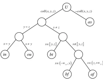
Ternary projective relations in R³ are almost totally equivalent to those in R². All the definitions presented in Table 1 stand in R² and R³ except the specialisation of the aside relation into rightside and leftside which is only possible in R². Indeed, the line joining the two reference points does not partition R³ into two parts anymore (as it was the case in R²). Therefore, it is impossible to refine the aside relation. The set of ternary relations among points aside, between, before, after, inside, outside is a JEPD set of relations in R³ (figure 1).

Table 1. The definitions of ternary projective relations among points in R³.

Name short name Definition drawing

Collinear coll(x,y,z) ∃line l x: ∈l y, ∈l z, ∈l Aside as(x,y,z)

¬

Inside in(x,y,z) x=y

∧

∧

∧

Nonbetween nonbt(x,y,z) coll(x,y,z)

∧

∧

∧

∧

yz ∈ −∞

After af(x,y,z) coll(x,y,z)

∧

∧

Fig. 1. A decision tree for the ternary projective relations among points in R³.

4. Quaternary projective relations between points in a 3D space

Another set of projective relations can be defined in R³ when considering one primary point and three reference points. Three non collinear points define one and only one plane in the space. Any plane in R³ is a hyperplane1 _{which means that it} divides the whole space in two regions, called halfspaces (HS). Depending on the order of the three reference points (clockwise or counterclockwise), the plane can be oriented in R³, which allows to distinguish between a positive and a negative halfspace (HS+, HS-). Based on this partition, one can define projective relations between a point and three reference points: these relations are therefore quaternary.

A point w lying in a plane defined by the three reference points x, y and z is said to be coplanar with x, y and z, we write copl (w,x,y,z). This coplanar relation can be refined depending on the relative position of the reference points. If the three reference points are collinear, then they define an infinity of planes that fill all the space. In such a degenerate case of coplanarity, we identify two quaternary projective relations called inside and outside. A point w is inside x, y and z if the three reference points are collinear and w belongs to the convex hull2 _{of x, y and z (which} corresponds to the segment joining the three points); otherwise, w is said to be outside x, y and z. These two relations are conceptually similar to inside and outside ternary relations. If the three reference points are aside then they generate two zones in the

1 _{A subset A of R}d

is an affine subspace if, for any distinct points x, y belonging to A, the straight line defined by x and y lies in A. Points, straight lines, planes, and R3 itself are the only affine subspace of R3. Their respective dimensions are 0, 1, 2 and 3. An affine subspace of dimension d-1 of Rd is named hyperplane.

2 _{The convex hull (CH) of two objects is formed by line segments joining each pair of objects’} points; these line segments belong to objects’ 1-transversals.

( , , ) coll x y z U in x=y y=z y z x ou ≠ y x [ as bt , bf af ( , , ) coll x y z ¬ ≠ ] y z ∈ x∈ −∞

(

)

(

)

reference plane; a zone defined by the convex hull of the three points and its complementary zone on the plane. A point w, coplanar with x, y and z, is said to be internal to x, y and z if it lies on the convex hull of x, y and z; otherwise it is said to be external to x, y and z. If the point w does not belong to a plane defined by the three reference points x, y and z, it is said to be non coplanar with x, y and z. This relation can be refined looking in which half-space the point w lies on. A point w which is non coplanar with x, y and z is said to be above x, y and z if it belongs to HSxyz

+

, or below x, y and z if it belongs to HSxyz

−

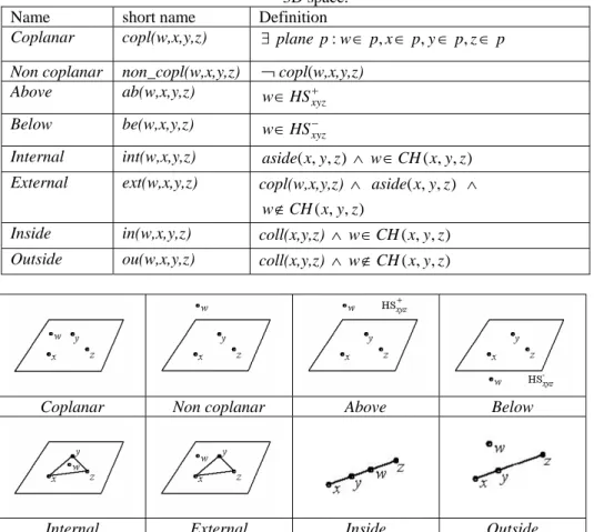
. Table 2 summarizes the quaternary projective relations between points in R³, which are illustrated in Figure 2.

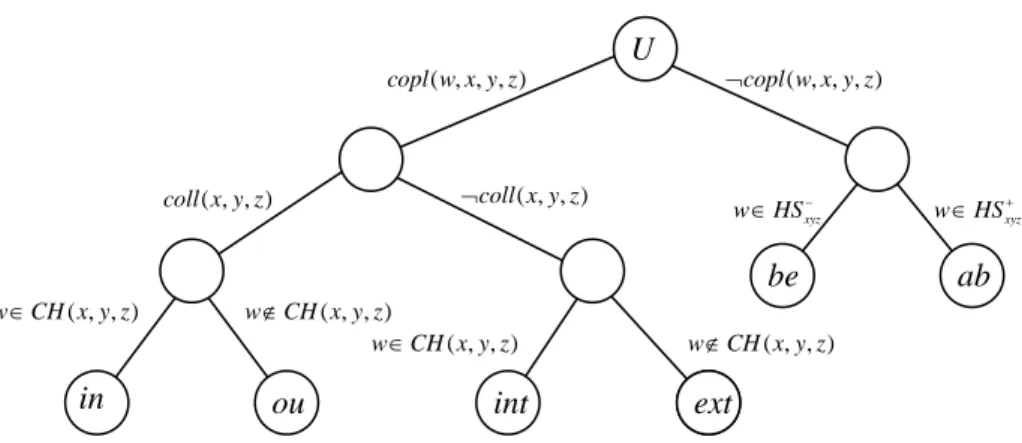
The set of quaternary relations among points above, below, internal, external, inside and outside is a JEPD set of relations in R³ (Figure 3).

Table 2. The definitions of quaternary projective relations among points in a

3D space.

Name short name Definition

Coplanar copl(w,x,y,z) ∃plane p:w∈p,x∈p,y∈p,z∈p Non coplanar non_copl(w,x,y,z)

¬

Above ab(w,x,y,z) _∈ + xyz HS w Below be(w,x,y,z) _∈ − xyz HS w

Internal int(w,x,y,z) aside(x,y,z) ∧ w∈CH(x,y,z)

External ext(w,x,y,z) copl(w,x,y,z) ∧ aside(x,y,z) ∧ ( , , )

w∉CH x y z

Inside in(w,x,y,z) coll(x,y,z) ∧ w∈CH(x,y,z)

Outside ou(w,x,y,z) coll(x,y,z) ∧ w∉CH(x,y,z)

Coplanar Non coplanar Above Below

Internal External Inside Outside Fig. 2. Quaternary projective relations among points in R³.

Fig. 3. A decision tree for the quaternary projective relations among points in R³.

5. Ternary projective relations between bodies in a 3D space

The importance of semantics of collinearity relies on the fact that modelling all ternary projective relations properties of spatial data can be done as a direct extension of such a property. The relation collinear among bodies can be introduced as a generalization of the same relation among points. Conceptually, collinearity relation between bodies in a 3D space does not differ from collinearity between regions in 2D. Among various definitions of collinearity [5], the most useful one is stated as follow:

Given three simple bodies A, B, C

∈

Let us examine the geometric realization of collinearity among bodies. Similar to points, where we had a degenerate case of collinearity for coincident reference points, we have a degenerate case of collinearity among bodies if reference bodies have non-disjoint convex hulls: a body A is always collinear to bodies B and C if the intersection is non-empty. If the intersection C ∩ is empty, we can identify a part of the space where a body A that is completely contained into it satisfies the relation collinear. Let us call this part of the space the collinearity subspace of B and C, Coll(B,C). Such a subspace can be built by considering all the lines that are intersecting both B and C. Knowing that a line that intersects a family of convex sets is called a 1-transversal [15], the collinearity subspace can be equally defined as the set of all 1-transversals to (convex hulls of) bodies B and C.

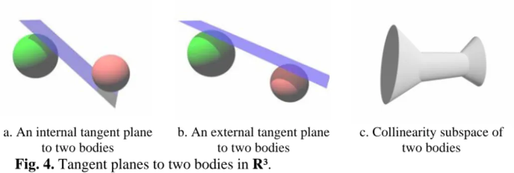
In R², the collinearity zone which is the 2D equivalent of the collinearity subspace was limited by the internal and external tangents of the two references objects (regions). In R³, the collinearity subspace is limited by two types of tangent planes; internal tangent planes that separates the two objects in different half-spaces (figure 4.a) and external tangent planes that leave the objects in the same half-space (figure 4.b). The intersection of all the half-spaces defined by internal tangent planes and

( , , , ) copl w x y z U int ext ( , , ) coll x y z ( , , ) w∈CH x y z ou ( , , ) w∈CH x y z w∉CH x y z( , , ) in ¬coll x y z( , , ) ( , , ) w∉CH x y z ¬ be ab ( , , , ) copl w x y z xyz w∈HS− w HSxyz + ∈

containing the first reference body, union with the intersection of all the half-spaces defined by internal tangent planes and containing the second reference body, union with the intersection of all the half-spaces defined by external tangent planes and containing the two reference objects define the collinearity subspace (figure 4.c).

a. An internal tangent plan b. An external tangent plane c. Collinearity subspace of

Fig anes to two bod

y definition, the convex hull of the union of two bodies is part of their collinearity su ich will b e to two bodies . 4. Tangent pl to two bodies ies in R³. two bodies B

bspace. The collinearity subspace of two bodies B and C (figure 5.a) can be subdivided in three parts; the convex hull of B∪C (figure 5.b) and two disjoint parts separated by the convex hull of B∪C wh e called collinear subspace

∞ −

CS (touching B) and collinear subspaceCS_+∞ (touching C) (figure 5.c).

a. Collinearity subspace of b. Convex hull of the union o c. Collinear subspaces

Fig o bodi

general, the part of the space where a body A that is c y contained into it sa

he definition ear can be extended to co co bodies B and C . 5. Partition of f B and C ace of tw ∞ − CS and CS_+∞ the collinear subsp es in R³.

In ompletel

tisfies a relation r is called the acceptance subspace of r. The collinearity subspace and all acceptance subspaces of relations are open sets: this corresponds to considering the interior of bodies in all the definitions of relations. This choice allows us to avoid limit cases: a point x in the boundary of body A that is falling in the boundary of an acceptance subspace does not influence the relation. If we had made the opposite choice, the point x would have contributed at the same time to the collinear and aside relations.

T of the relation collin mplex bodies by

nsidering the convex hulls of the reference objects in place of the reference objects. The definition of collinear together with other projective relations for bodies is given in Table 3. Besides each definition, also the corresponding acceptance subspace is

Table 3. The definitions of projective relations among regions.

relation Defi

given. The relation collinear, in the case the two reference bodies have not disjoint convex hulls, can be refined in two relations that are called inside and outside. The relations between and nonbetween are refinements of the relation collinear, in the case the two reference bodies have disjoint convex hulls. The relation nonbetween can be refined in the two relations before and after, respectively.

nition Acceptance subspace

coll(A,B,C) ∀ ∈ °x A [∃y∈CH B( )° [∃ ∈z CH ° [coll(x,y ]]] ∪ CH B C ( )C ,z) Coll(B,C) = (CS_−∞)° (CS_+∞)°∪ ( ( ∪ ))° as(A,B,C) x A° [∀ ∈y [∀ ∈z C C ° [as(x,y,z ] side(B =(R³ - Coll(B,C ∀ ∈ CH B( )° ( ) H )]] A ,C) ))° in(A,B,C) CH( )B ∩CH C( )≠ ∅ ∧ ( ( )) A° ⊆ CH B∪C ° Inside(B,C) = (CH B( ∪C))° ou(A,B,C) CH B( )∩CH C( )≠ ∅ ∧ ( ( )) A° ∩ CH B∪C = Outside(B,C) = R³ - CH B( ∪C) ∅ bt(A,B,C) CH(B)∩CH(C)=∅ ∧ ( ( )) A° ⊆ CH B∪C ° Between(B,C) = (CH(B∪C))° nonbt(A,B,C) Coll(A,B,C) ∧ C ∅ ( ) ( ) CH B ∩CH = ∧ A° ∩CH Between( CS_−∞)°∪ (B∪C)= ∅ Non B,C) = ( (CS_+∞)° bf(A,B,C) CH B( )∩CH C( )=∅ ∧ A° ⊂CS_−∞ Before(B,C) ( = CS_−∞)° af(A,B,C) CH B( )∩CH( )C = ∅ ∧ A° ⊂CS_+∞ After(B,C) = (CS_+∞)°

imilarly to ternary projectiv tions between regions in R² [4] se the basic rel

empty su

∩Before(B,C), A∩Betwe C

S e rela , we u

ations aside, between, before, after, inside, and outside to build a model for projective relations between three bodies of R³. The subspaces corresponding to the first four relations make a partition of the space R³ in the case the two reference bodies have disjoint convex hulls. If the two reference bodies have non disjoint convex hulls, the space is partitioned in two subspaces, corresponding to relations inside and outside.

Let us consider /non-empty intersections of a body A with the four bspaces:

(A en(B, ), A∩After(B C), A, ∩Aside(B,C

value 0 indicates an e n, while a value 1 indicates a n p int

))

A mpty intersectio on-em ty

ersection. The 4-intersection can have 24–1 different configurations. Each configuration corresponds to a projective relation among three bodies A, B, and C,

It is possible to extend the concept of quaternary relations between points in R³ to bodies. The concept of coplanarity between four bodies can be introduced as a generalisation of the same relations among points. Following the same reasoning as when defining collinearity among bodies, we propose the following definition of coplanarity among bodies:

( ) ( )

CH B ∩CH C = ∅

( ) ( )

CH B ∩CH C ≠ ∅

∩

where . Four values equal to zero does not correspond to a relation. For , we consider the following 2 intersections:

(A Inside(B,C), A∩Outside(B,C))

which can assume the values (0 1), (1 0), and (1 1). Overall, we obtain a model that is able to distinguish among a set of 18 ternary projective relations among three bodies of R³, which are JEPD.

We can use a linear notation for the relation, by listing 6 bits that represent the intersection of body A with Before(B,C), Between(B,C), After(B,C), Aside(B,C), Inside(B,C), Outside(B,C).

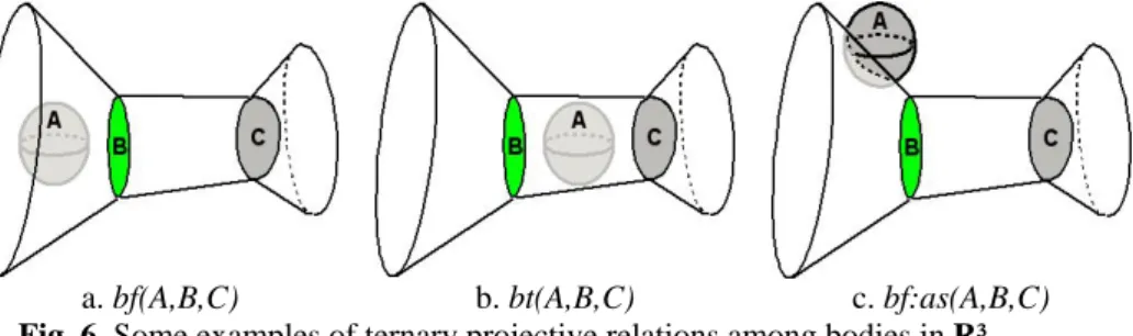
In this notation, the basic relations are expressed as follows: bf(A,B,C) = (1 0 0 0 | 0 0), bt(A,B,C) = (0 1 0 0 | 0 0), af(A,B,C) = (0 0 1 0 | 0 0), as(A,B,C) = (0 0 0 1 | 0 0), in(A,B,C) = (0 0 0 0 | 1 0), ou(A,B,C) = (0 0 0 0 | 0 1). Other relations correspond to cases with more than one non-empty value: for example, a relation that is a combination of two basic relations, such as a “before and aside”, is indicated as: bf:as(A,B,C) = (1 0 0 1 | 0 0). Figure 6 contains three examples of ternary projective relations among bodies in R³.

a. bf(A,B,C) b. bt(A,B,C) c. bf:as(A,B,C) Fig. 6. Some examples of ternary projective relations among bodies in R³.

6. Quaternary projective relations between bodies in a 3D space

Let us examine the geometric realization of coplanarity among bodies. Similar to points where we had a degenerate case of coplanarity for collinear reference points, we have a degenerate case of coplanarity among bodies if reference bodies have at least a triplet of collinear points. If there exists at least one triplet of collinear points x, y and z, the relation coplanar with any point w of R³ is true; the coplanar subspace in

w A

this case is R³ itself. Otherwise, we can identify a part of the space where a body A that is completely contained into it satisfies the relation coplanar. Let us call this part of the space the coplanarity subspace of B, C and D, Copl(B,C,D). Such a subspace can be built by considering all the planes that are intersecting B, C and D. Knowing that a plane that intersects a family of convex sets is called a 2-transversal [15], the coplanarity subspace can be equally defined as the set of all 2-transversals to (convex hulls of) bodies B, C and D.

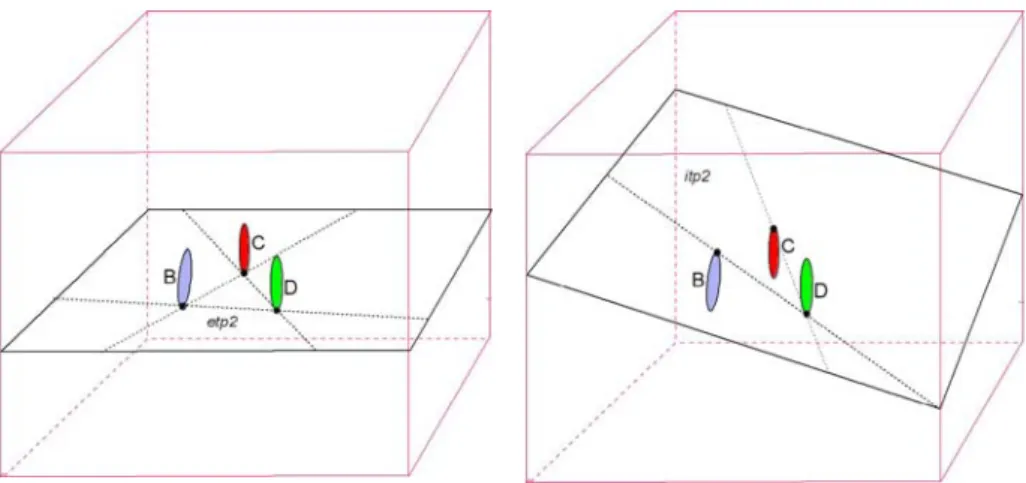
Like the collinear subspace, the coplanarity subspace can be seen as the intersection of half-spaces defined by internal tangent planes combined with the intersection of half-spaces defined by external tangent planes and containing the three reference objects. In this case, internal tangent planes separate two objects in one half-space and the third one in the other half-half-space and external tangent planes leave the three objects in the same half-space. By definition, there are 6 internal tangents planes and 2 external tangents planes to three bodies that do not contain triplets of collinear points [12]. Figure 7 shows an external tangent plane (etp2) and an internal tangent plane (itp2) of three bodies (B, C and D). The coplanar subspace partitions R³ in two distinct subspaces. Considering an order among the reference bodies (clockwise or counterclockwise), it is possible to consider a general orientation of the coplanarity subspace in R³. One ends up with three subspaces, the coplanar subspace, the non-coplanar subspace NCS+(B,C,D) and the non-coplanar subspace NCS-(B,C,D)).

a. An external tangent plane (etp2) of B, C and D

a. An internal tangent plane (itp2) of B, C and D

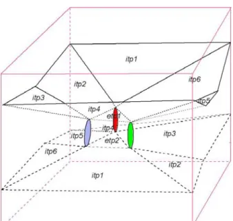
Fig. 8. Combination of internal and external tangent planes to three bodies in R³.

Figure 8 illustrates the combination of internal and external tangent planes. There are six internal tangent planes called itp1, …, itp6 and two external tangent planes etp1 and etp2. The six internal tangent planes form the top part of the coplanarity subspace (Figure 9.a) with etp1 and the bottom part of the coplanarity subspace (Figure 9.a) with etp2. Figure 9.b represents the corresponding coplanarity subspace.

a. Top and bottom of the coplanarity subsapce

b. Corresponding coplanarity subspace

Fig. 9. Coplanarity subspace of three bodies in R³ (bodies are not represented).

Knowing that the convex hull of the union of three bodies is part of their coplanarity subspace, one can partition further the coplanarity subspace of three bodies B, C and D considering the convex hull of B∪ ∪C D and its complement in

B∪ ∪C D B∪ ∪C D

the coplanarity subspace. These two subspaces are respectively called Internal(B,C,D) and External(B,C,D).

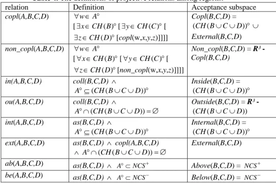
The definition of the relation coplanar can be extended to complex bodies by considering the convex hulls of the reference objects in place of the reference objects. The definition of coplanar together with other quaternary projective relations for bodies is given in Table 4. Besides each definition, also the corresponding acceptance subspace is given. If there is no plane joining any points of A, B, C and D, body A is non coplanar with B, C and D. The relation coplanar, in the case the three reference bodies are collinear, can be refined in two relations that are called inside and outside, depending if body A is included or not in the convex hull of . Otherwise, the coplanar relation can be refined into internal and external relations depending if body A is included or not in the convex hull of . The non coplanar relation can be also specialised into above and below relations depending in which non-coplanar subspaces body A is included.

Table 4. The definitions of projective relations among regions.

relation Definition Acceptance subspace

copl(A,B,C,D) ∀ ∈ °w A ( ) [∃ ∈x CH B °[∃ ∈y CH C( )° ( ) z CH D ∃ ∈ ° (CH B( ∪ ∪C D))° ∪ [ [copl(w,x,y,z)]]]] Copl(B,C,D) = External(B,C,D) non_copl(A,B,C,D) ∀ ∈ °w A ( ) [∀ ∈x CH B °[∀ ∈y CH C( )° ( z CH ∀ ∈ [ [non_copl(w,x,y,z)]]]] ) D° Non_copl(B,C,D) = R³ - Copl(B,C,D) in(A,B,C,D) coll(B,C,D) ∧ ( ( )) A° ⊆ CH B∪ ∪C D ° (CH B( ∪ ∪C D) Inside(B,C,D) = )° ou(A,B,C,D) coll(B,C,D) ∧ ( ( )) A° ∩ CH B∪C∪D = ∅ (CH B( ∪ ∪C D)) Outside(B,C,D) = R³ - int(A,B,C,D) as(B,C,D) ∧ ( ( )) A° ⊆ CH B∪ ∪C D ° ))° Internal(B,C,D) = (CH B( ∪ ∪C D ext(A,B,C,D) as(B,C,D) ∧ copl(A,B,C,D)

∧ A° ∩(CH B( ∪ ∪C D))= ∅

External(B,C,D) ab(A,B,C,D) _{as(B,C,D) ∧ A° ⊂NCS}+ _{Above(B,C,D) =}

NCS+

be(A,B,C,D) _{as(B,C,D) ∧ A° ⊂NCS}−

Below(B,C,D) = NCS−

Like for the ternary projective relations, the all set of quaternary relations between four bodies can be obtained based on empty/non-empty intersections of the primary body A with the subspaces which satisfy the basic quaternary relations.

Let us consider empty/non-empty intersections of a body A with the four subspaces:

( ) ( ) ( ) CH B ∩CH C ∩CH D = ∅

( ) ( ) ( )

CH B CH C CH D

The 4-intersection can have 24–1 different configurations. Each configuration corresponds to a quaternary projective relation among four bodies A, B, C and D,

where . Four values equal to zero does not

correspond to a relation. For ∩ ∩ ≠ ∅

∩ ∩

, we consider the following 2 intersections:

(A Inside(B,C,D), A Outside(B,C,D))

which can assume the values (0 1), (1 0), and (1 1). Overall, we obtain a model that is able to distinguish among a set of 18 quaternary projective relations among three bodies of R³, which are JEPD.

We can use a linear notation for the relation, by listing 6 bits that represent the intersection of body A with Internal(B,C,D), External(B,C,D), Above(B,C,D), Below(B,C,D), Inside(B,C), Outside(B,C).

In this notation, the basic relations are expressed as follows: int(A,B,C,D) = (1 0 0 0 | 0 0), ext(A,B,C,D) = (0 1 0 0 | 0 0), ab(A,B,C,D) = (0 0 1 0 | 0 0), be(A,B,C,D) = (0 0 0 1 | 0 0), in(A,B,C,D) = (0 0 0 0 | 1 0), ou(A,B,C,D) = (0 0 0 0 | 0 1). Other relations correspond to cases with more than one non-empty value: for example, a relation that is a combination of two basic relations, such as a “internal and below”, is indicated as: int:be(A,B,C,D) = (1 0 0 1 | 0 0). Figure 10 contains four examples of quaternary projective relations among bodies in R³.

c. ab(A,B,C,D) d. ext:ab(A,B,C,D) Fig. 10. Some Examples of quaternary projective relations among bodies in R³

(bodies are not represented).

In this paper, we have first presented ternary projective relations among points and among bodies in R³. The resulting model uses the concept of collinearity among bodies, which has been extended from previous work on points and regions in R². The points’ model provides a set of six JEPD ternary relations in R³ instead of seven in

R²: aside, between, before, after, inside and outside. The bodies’ model provides a set

of eighteen JEPD ternary relations in R³ based on the same basic six relations. As a second part, considering three reference objects, the concept of coplanarity has been introduced. In this case, the points’ model provides a set of six JEPD quaternary relations in R³: above, below, internal, external, inside and outside, when the bodies’ model provides a set of eighteen JEPD ternary relations in R³ based on the same basic six relations. Formal definitions and models to express all these relations have been proposed.

7. Conclusions

The study of the formal properties of relations and the development of a reasoning system is a future major issue. Development of algorithms to compute such 3D relations is needed and will complete the work already done for ternary relations among points and regions in R². More generally, the study of properties of such relations will be important for optimizing the computation of more complex kinds of queries and for integrating ternary and quaternary projective relations as operators in a spatial database system. Finally, work needs to be done to “map” these concepts and models to specific 3D environments; e.g. to map the bottom of a coplanarity subspace on the topographic surface and use projective relations in the corresponding deformed space.

References

1. Bartie, P.J. and W.A. Mackaness, Development of a Speech-Based Augmented Reality System to Support Exploration of Cityscape. Transactions in GIS, 2006. 10(1): p. 63-86.

2. Bennett, B., et al., Region-based qualitative geometry. 2000, University of Leeds, School of Computer Studies, LS2 9JT, UK. Technical Report 2000.07.

3. Billen, R. and E. Clementini. Introducing a reasoning system based on ternary projective relations. in Developments in Spatial Data Handling, 11th International Symposium on Spatial Data Handling. 2004. Leicester, UK: Springer-Verlag. p. 381-394.

4. Billen, R. and E. Clementini. A model for ternary projective relations between regions. in EDBT2004 - 9th International Conference on Extending DataBase Technology. 2004. Heraklion - Crete, Greece: Springer-Verlag. p. 310-328.

5. Billen, R. and E. Clementini, Semantics of collinearity among regions, in OTM Workshops 2005 - 1st Int. Workshop on Semantic-based Geographical Information Systems (SeBGIS'05), R. Meersman, Editor. 2005, Springer-Verlag: Agia Napa, Cyprus. p. 1066-1076.

6. Clementini, E. and R. Billen, Modeling and computing ternary projective relations between regions. IEEE Transactions on Knowledge and Data Engineering, 2006. 18(6): p. 799-814.

7. Coxeter, H.S.M., Projective Geometry, 2nd ed. 1987, New York: Springer-Verlag.

8. Freksa, C., Using Orientation Information for Qualitative Spatial Reasoning, in Theories and Models of Spatio-Temporal Reasoning in Geographic Space, A.U. Frank, I. Campari, and U. Formentini, Editors. 1992, Springer-Verlag: Berlin. p. 162-178.

9. Gapp, K.-P. From Vision to Language: A Cognitive Approach to the Computation of Spatial Relations in 3D Space. in Proc. of the First European Conference on Cognitive Science in Industry. 1994. Luxembourg. p. 339-357.

10. Hernández, D., Qualitative Representation of Spatial Knowledge. Lecture Notes in Artificial Intelligence. Vol. LNAI 804. 1994, Berlin: Springer-Verlag.

11. Klein, F., Vergleichende Betrachtungen über neuere geometrische Forschungen. Bulletin of the New York Mathematical Society, 1893. 2: p. 215-249.

12. Lewis, T., B. von Hohenbalken, and V. Klee, Common supports as fixed points. Geometriae Dedicata, 1996. 60(3): p. 277-281.

13. Ligozat, G.F. Qualitative Triangulation for Spatial Reasoning. in European Conference on Spatial Information Theory, COSIT'93. 1993. Elba Island, Italy: Springer Verlag. p. 54-68.

14. Scivos, A. and B. Nebel, The Finest of its Class: The Natural Point-Based Ternary Calculus for Qualitative Spatial Reasoning, in Int. Conf. Spatial Cognition. 2004, Springer. p. 283-303.

15. Wenger, R., Progress in geometric transversal theory, in Advances in Discrete and Computational Geometry, B. Chazelle, J.E. Goodman, and R. Pollack, Editors. 1998, Amer. Math. Soc.: Providence. p. 375-393.

16. Zlatanova, S., 3D GIS for Urban Development. 2000, University of Graz - ITC.