HAL Id: tel-01123747
https://pastel.archives-ouvertes.fr/tel-01123747
Submitted on 5 Mar 2015HAL is a multi-disciplinary open access archive for the deposit and dissemination of
sci-L’archive ouverte pluridisciplinaire HAL, est destinée au dépôt et à la diffusion de documents
Ralf Kohlhaas
To cite this version:
Ralf Kohlhaas. Feedback Control of Collective Spin States for Atom Interferometry. Other [cond-mat.other]. Institut d’Optique Graduate School, 2014. English. �NNT : 2014IOTA0001�. �tel-01123747�
´
ECOLE DOCTORALE ONDES ET MATI`
ERE
Discipline : Physique
TH`ESE
pour l’obtention du grade de Docteur en science de l’Institut d’Optique Graduate School
pr´epar´ee au Laboratoire Charles Fabry
soutenue le 17/01/2014
par
Ralf KOHLHAAS
Feedback Control of Collective Spin
States for Atom Interferometry
Composition du jury :
M. A. Aspect Directeur de th`ese M. R. Kaiser Rapporteur
M. E. Rasel Rapporteur M. S. Bize Examinateur M. J.-M. Courty Examinateur M. P. Pillet Pr´esident du jury M. P. Bouyer Membre invit´e M. A. Landragin Membre invit´e
Introduction 1
1. Collective Spin States and Generalized Quantum Measurements 7
1.1. Introduction . . . 7
1.2. Collective Spin States . . . 8
1.2.1. Bloch Sphere . . . 8
1.2.2. Coherent Spin States . . . 10
1.2.3. Spin Squeezed States . . . 14
1.2.4. Evolution under Unitary Operations . . . 16
1.3. Generalized Quantum Measurements . . . 19
1.3.1. Motivation. . . 19
1.3.2. Ideal Projective Measurement . . . 21
1.3.3. Generalized Measurement Operators . . . 22
2. Preparation of Cold Atomic Samples 33 2.1. Introduction . . . 33
2.2. Vacuum System and Magneto-Optical Trap . . . 34
2.3. Cavity Enhanced Optical Dipole Trap. . . 37
2.3.1. Motivation for Optical Cavity . . . 37
2.3.2. Geometrical Description . . . 38
2.3.3. Optical Properties . . . 39
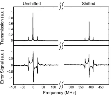
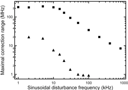
2.3.4. Laser Stabilization by Serrodyne Modulation . . . 41
2.4. Dipole Trap Loading . . . 50
2.4.1. AC Stark Shift . . . 50
2.4.2. Loading Scheme. . . 50
2.4.3. Atom Number and Trap Lifetime . . . 52
2.5. Evaporation and Bose-Einstein Condensation . . . 53
2.5.1. Motivation. . . 53
2.5.2. Evaporation and Condensation . . . 54
2.5.4. Outlook with BEC . . . 58
2.6. Preparation of Internal States . . . 58
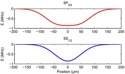
2.6.1. Cancellation of Differential Light Shift . . . 58
2.6.2. State Purification . . . 63
3. Nondestructive Detection System 67 3.1. Introduction . . . 67
3.2. FM Spectroscopy . . . 68
3.2.1. Operation Principle . . . 68
3.2.2. Detection Noise . . . 69
3.2.3. Dispersive Probing . . . 71
3.2.4. Stability Against Path Length Fluctuations . . . 73
3.3. Experimental Setup . . . 73
3.3.1. Optical Bench . . . 73
3.3.2. Photodiode Characteristics . . . 75
3.4. Direct Population Measurement . . . 76
3.4.1. Probe Scheme . . . 77
3.4.2. Suppression of Probe Light Shift . . . 79
3.4.3. Balancing of Decoherence . . . 81
3.4.4. Maximization of SNR for a Given Decoherence . . . 84
3.5. FM Spectroscopy as a Calibration Tool . . . 86
3.5.1. Characterization of Microwave Source . . . 87
3.5.2. Real Time Observation of Rabi Oscillations . . . 88
3.5.3. Observation of Atomic Projection Noise . . . 89
4. Feedback Control of Collective Spin States 95 4.1. Introduction . . . 95
4.2. General Description of the Control Problem . . . 96
4.2.1. Decoherence by Collective Noise . . . 96
4.2.2. Feedback Control . . . 97
4.2.3. Feedback Efficiency . . . 98
4.3. Experimental Implementation . . . 99
4.3.1. Experimental Setup. . . 99
4.3.2. Study of Binary Collective Noise . . . 101
4.3.3. Study of Analog Collective Noise . . . 113
5. Atomic Phase Lock 121 5.1. Introduction . . . 121
5.2. Atomic Clock Operated with the Standard Ramsey Protocol . . . . 122
5.2.1. Operation Principle . . . 122
5.2.2. Stability Limits . . . 123
5.2.3. Dick Limit . . . 125
5.3. Concept of Atomic Phase Lock . . . 127
5.3.1. The Proposal by N. Shiga and M. Takeuchi . . . 127
5.3.2. Our Feedback Protocol . . . 131
5.4. Experimental Results . . . 134
5.4.1. Real Time Observation of the Phase in a Ramsey Interfer-ometer . . . 134
5.4.2. Stabilization of LO Phase on Atomic Phase . . . 136
5.4.3. Full Feedback Scheme . . . 138
5.5. Variations of the Feedback Protocol . . . 142
5.5.1. Feedback on the Atomic Phase . . . 142
5.5.2. Auxiliary Atomic Ensemble . . . 143
5.6. Other Proposals to Increase Interrogation Time in Atomic Clocks . 144 5.7. Application of Atomic Phase Lock to Other Sensors . . . 145
5.7.1. Gravimeter . . . 146
5.7.2. Gyroscopes . . . 147
6. Conclusion 149 Appendix A. Weak Measurements of CSSs with Postselection 153 A.1. Presentation of a Simple Example . . . 153
A.2. Calculation with Standard Quantum Mechanics . . . 155
A.3. Calculation with Time Symmetric Quantum Mechanics . . . 155
Appendix B. Level Structure of Rubidium-87 157 Appendix C. Atomic Polarizabilities and Branching 159 C.1. Polarizability . . . 159
C.2. Branching Ratios from Spontaneous Emission . . . 160
Appendix D. Dephasing in Dipole Trap 161 Appendix E. State Parameters Before and After Feedback 163 E.1. Coherence . . . 163
E.3. Von Neumann Entropy . . . 165
Appendix F. Dick Effect under 1/f-Noise 167
On 22 October 1707 four English warships, the Association, Eagle, Firebrand and Romney, hit ground in a foggy night at the Scilly Islands on the English coast and sank. Two thousand lives were lost. The accident would have been avoidable - had only the crews known their longitude. At that time, no reliable method existed to determine the longitude of a ship. An astronomical solution seemed most promising and had led before to the construction of the astronomical observatories in Greenwich and Paris, but without any success so far for the longitude problem.
In 1714, the English government issued the “longitude act”, awarding 20.000 pounds (the equivalent of several million euros today) to anybody who could determine a longitude within half a degree. Although everybody expected an astronomical solution, the final answer turned out to be much simpler: a good clock. With the ability to take a timekeeper with you, and the possibility to determine the local time over the position of the sun, the time difference to the home port could be calculated.
At the beginning of the 18th century, the best available clocks went wrong by several seconds a day and were far from being transportable. Leading scientists including Isaac Newton considered the determination of longitude by a portable timekeeper hopeless. They were proven wrong by John Harrison, a former carpenter and then clockmaker. He built in a life work from 1713 to 1776 transportable clocks which went only wrong in a fraction of a second over a whole month, and his portable clock, called the chronometer, became the standard for determining longitude. The stability of the chronometer was owed to a careful choice of materials and new inventions (for example, it used bimetallic strips and caged roller bearings, both invented by John Harrison), and became the standard for the determination of longitude in the navy1.
1Nevertheless, John Harrison has never been awarded the official longitude act prize as a result of political quarrels. A very good book about the history of the chronometer and the longitude act can be found in [Sobel 07].
Today’s best clocks are based on the laws of quantum mechanics. They go wrong only by a fraction of a second over the age of the universe, or in other words have an instability of 10−18 [Hinkley 13,Bloom 13]. Quantum mechanics is based on a set of rules which are not common with the classical world we face every day. First, we know the energy can only exist in fixed packages, so called quanta. This gives an exact building plan for single atoms, and because its constituents (protons, neutrons and electrons) are always the same, all atoms with the same number of constituents are the same as well. The difference between the energy levels ∆E = E2− E1 in atoms can serve then as an absolute frequency reference via Planck’s law ∆E =~ω, where ~ = 2π 6.626 × 10⁻³⁴ Js is the reduced Planck’s constant and ω an angular frequency.
Another property of quantum mechanics is that objects very well isolated from their environment can be prepared, and survive, in a superposition of different states. A single electron can behave as if it travels two paths at the same time, as if it were an electromagnetic wave. In an atomic interferometer, it is the internal or external states of atoms which are put in superposition states. Dedicated protocols, such as the Ramsey scheme [Ramsey 80], use the creation and combination of superposition states for the measurement of physical quantities such as frequencies, accelerations and magnetic fields [Berman 97].
In an atomic clock, the frequency of a macroscopic oscillator (e.g. a quartz crystal) is periodically compared to a transition frequency of an atomic species. This oscillator (also called local oscillator LO) is then stabilized on the atomic transition frequency. The frequency of the classical oscillator can be measured with a counter and is used for the definition of time. The stability of the LO improves when its frequency is compared to the frequency of the atomic reference for a longer interval. But this interrogation time is usually limited: during the interrogation, the atoms are in a superposition of states, and the superposition can be destroyed under the influence of the environment. This process is called decoherence, and the initial ability of the atomic states to interfere, their coherence, is reduced.
The most precise atomic clocks are based on atomic ensembles, and the main decoherence source is the frequency noise of the free running LO itself. Noise of this kind is called “collective noise” because it affects all atoms in the same
resonators is a target pursued by a large number of groups around the world, and tremendous progress has been made with instabilities down to the 10−16 level at one second [Jiang 11, Thorpe 11, Kessler 12]. However, the interrogation times of optical atomic clocks have remained below a fraction of a second. In trapped microwave clocks, the recently found spin-self rephasing of atoms [Deutsch 10] could potentially enable interrogation times of tens of seconds, but the quality of the existing microwave oscillators does not allow it.
An alternative solution to protect a quantum system against decoherence is to measure it, and to apply feedback either on the quantum system itself or on its environment. Another feature in quantum mechanics comes into play here, the property that measuring a quantum system also modifies it. The control laws in quantum mechanics can be therefore very distinct from classical control laws and have been subject to extensive theoretical efforts [Doherty 00, Lloyd 00, Ahn 02, Mancini 07] and first experimental demonstra-tions [Armen 02,Smith 02,Gillett 10]. Only recently, for the first time a quantum state, a photon number state, was permanently stabilized against decoherence [Sayrin 11]. Experiments on superconducting qubits show fast progress in the same direction, with the real time stabilization of Rabi-oscillations [Vijay 12] and quantum measurements with variable measurement strength [Hatridge 13]. The main application area is likely to be here quantum information processing.
In this thesis, we bring the concept of feedback on a quantum system to atomic interferometers. From a first glance, this approach might appear to be a bad idea. The atoms in the interferometer act as a probe, and as such should by no means be disturbed during their evolution. But simply measuring the atoms does exactly that. However, there is a way out of this problem: atomic ensembles can be measured gently, or “weakly”, to provide significant information while changing the quantum state only very little [Aharonov 88, Smith 04, Aharonov 10]. This makes it possible to use classical feedback control for the collective quantum system. We will show that in this way decoherence by collective noise in atomic interferometers can at least be partially removed. Our experimental results and feedback protocols indicate a realistic potential for the improvement of atomic sensors by active feedback control.
This is the third PhD thesis handed in on the experimental apparatus after Simon Bernon [Bernon 11a] and Thomas Vanderbruggen [Vanderbruggen 12]. As a postdoc, Andrea Bertoldi took both part in the experimental work and later took over a large part of the direction of the experiment. Arnaud Landragin and Philippe Bouyer were the scientific directors of the experiment and Alain Aspect as the head of the Atom Optics group and my PhD supervisor advised the performed work. Etienne Cantin is a new PhD student who contributed to the last experimental results in this manuscript. The results presented in this manuscript have been already partially covered by our previous publications [Bernon 11b, Kohlhaas 12, Vanderbruggen 13], and results from the last two chapters remain to be published. The feedback protocols in the last chapter have been submitted for a patent application.
The experimental setup as it already existed at the beginning is described only briefly, as a basis for the understanding of the further work. Detailed calculations or derivations will only be shown if they are original and are otherwise cited. For most explanations, at first a simple picture is given before a more formal description. The manuscript is organized in 5 chapters. Below a summary of the chapters is given.
Chapter 1. In this chapter, the main theoretical concepts used in the the-sis are introduced. The Bloch sphere picture describes the structure and evolution of the internal states of atomic ensembles. The formulation in the Dicke state basis allows for arbitrary state transformations. Generalized quantum measurements are introduced as a generalization of the ideal pro-jective measurement. The concept of generalized quantum measurements on collective spin states is explained, and the special case of weak measurements is discussed.
Chapter 2. The experimental setup for the preparation of cold atomic clouds is presented. It contains several unique features, including a dipole trap in an optical cavity in butterfly configuration. We present novel tech-nological solutions such as a new stabilization scheme of a laser on a cavity, and the production of a Bose-Einstein condensate with a cavity-enhanced dipole trap. We show a new procedure to engineer the atomic light shift on an optical transition and demonstrate how we prepare a pure internal state of a dense ensemble of atoms with optical methods.
frequency modulation spectroscopy, and is the only system where the popu-lation difference of two non-magnetic atomic states can be read out nonde-structively with a single optical beam. We show how to set the couplings of the light to the atomic levels correctly, avoid light shifts from the probe and balance the spontaneous emission to the probed states. The beam waist of the beam is optimized for a maximal signal-to-noise ratio. We show some first results with the nondestructive detection system such as the real time observation of Rabi oscillations.
Chapter 4. We present the feedback control of the collective internal states in an atomic ensemble. All atoms are prepared in a superposition state of two atomic levels, and artificial noise is applied on the atoms. The state of the atoms is measured weakly, and feedback with coherent manipulations restores partly the initial state. We study theoretically different parameters over which the feedback efficiency can be characterized, and choose experimentally to observe the output coherence of the state. We show that there is a trade-off between the information and the perturbation from the measurement. Different noise and feedback scenarios are studied. The work in this chapter represents the first demonstration of the protection of a superposition state against decoherence with feedback control, although only for the case of an ensemble and collective noise.
Chapter 5. We stabilize the phase of a LO in an atomic clock on the phase of a superposition state of the atoms, as it was proposed in [Shiga 12] to improve atomic clocks. The scheme is equivalent to remove the decoherence of the atoms by feedback on the environment, which is here the LO. We find a drawback in the original phase lock scheme proposed in [Shiga 12], and develop a new feedback protocol. The experimental results raise realistic hopes that our methods could be used to improve atomic clocks. It is shown that our feedback protocol is versatile, and could be applied to other atomic interferometers such as gravimeters. The work in this chapter shows for the first time the stabilization of a classical object to a quantum system in a superposition state, which could have widespread applications for precision measurements.
The content of this manuscript is more focused on new ideas and techniques than on pushing an instrument to its limits. The hope is expressed here that the reader
will find some of it interesting, and that perhaps part of the work will be the basis for further research.
1.1. Introduction
The central goal of this thesis is to demonstrate how trapped coherent atomic ensembles can be measured nondestructively and controlled via feedback, and to investigate if this could lead to an improvement of atomic interferometers. In this chapter, the theoretical basics for this work are given. The trapped atoms that we use can be approximated by a two-level system, one of the most basic systems in quantum mechanics. A useful tool to illustrate the evolution of a single two-level system is the Bloch sphere model, which is introduced in Section 1.2.1. In this model, the state of a two-level system becomes a pseudo-spin, in analogy to a real spin vector of for example a magnetic moment.
Since we work with an ensemble of atoms, a generalization of the Bloch sphere picture to many atoms is needed. The simplest collective state of an ensemble of two-level atoms, a coherent spin state (CSS), is then introduced in Section 1.2.2. In a CSS, all atoms are in the same pure internal state, and all single pseudo-spins can be added up to from a giant collective spin. Although we do not work with entangled states, the concept of a spin squeezed state (SSS) is introduced in Section 1.2.3. In a spin squeezed state, a constraint is imposed on the collective spin state and the indistinguishable individual spins are correlated. Since a SSS can be the result of a partially projective quantum measurement, it is a good starting point for the introduction of generalized quantum measurements on collective atomic states.
To actively control any system, one has to measure it. In quantum mechanics, the measurement process itself can modify the system of interest. The prime example here is an ideal projective measurement, where before the measurement a particle can be in a superposition of two states, and after the measurement it is only in one of the two states. The projective measurement is the textbook example
of a quantum measurement, but unfortunately often also the only type of quantum measurement taught to students of quantum mechanics. As a matter of fact, the ideal projective measurement does not exist in practice, since any measurement always contains some residual noise. The experiments which have so far come the closest to an ideal projective measurement were performed on microwave photons measured by Rydberg atoms [Guerlin 07] and on trapped ions [Hume 07]1. The main results of this thesis will rely on the fact that a measurement on a quantum system does not necessarily have to be projective. In fact, our goal will be to project the measured state as little as possible while still obtaining sufficient information to perform feedback on the atoms. The concept of general quantum measurements is introduced in Section 1.3 with the Kraus operator formalism, which gives the rules to formulate general quantum measurements. We apply the concept then to collective atomic states in Section1.3.3.5, and define the important parameters for the measurement process. The results from this last section will then be repeatedly used throughout this manuscript. The feedback control of collective atomic states is not treated in this chapter, and is developed alongside with the experimental results in Chapter 4.
1.2. Collective Spin States
1.2.1. Bloch Sphere
The Bloch sphere representation has been introduced for the description of nuclear magnetic resonance (NMR) phenomena, and named in honor of F. Bloch for his pioneering work on nuclear induction [Bloch 46]. In NMR, the real nuclear magnetic spin with a vector M in an external magnetic field B is the Bloch vector. It can have any direction in space, and the Bloch sphere is formed by the set of all spin directions. By going in the rotating frame of a transverse oscillating magnetic field, an easy picture for manipulations of the nuclear spin can be obtained, and this is still the basic model in NMR experiments. It was later pointed out by R. Feynman and coworkers [Feynman 57] that the Bloch sphere model can be generalized to other systems containing at least two
1The atomic state of 27Al+ could be measured in [Hume 07] with a certainty of 99.94%. The development of measurement tools for ions and microwave photons were one reason for the Nobel prize in Physics in 2012 to S. Haroche and D. Wineland.
Figure 1.1.: Introduction to the Bloch sphere picture. The state of a two-level system can be represented as a spin vector on the Bloch sphere. The z-axis corresponds to the population difference and the x− y plane designates the phase between the superposition state referenced on the phase of a local oscillator (LO). The spin direction is described with the azimuthal angle ϕ and the polar angle θ.
distinct levels. A single atom containing two quantized energy levels can then be represented as a pseudo-spin on the Bloch sphere. The same holds as well for superposition states of the polarization of a photon [O’Brien 07], but also for classical systems such as coupled modes of a mechanical oscillator [Faust 13]. The Bloch sphere is a useful tool to describe atomic interferometers, notably atomic clocks. The state of a single two-level system can be described as
|φ⟩ = a |0⟩ + be−iωatt|1⟩ , (1.1)
where a and b are the probability amplitudes to be in state |0⟩ or |1⟩ and it holds
|a|2
+|b|2 = 1. We will later identify in the experimental work |0⟩ and |1⟩ to be two hyperfine ground states of 87Rb. The frequency ωat comes from the energy difference of the two energy states with E =~(ω1− ω0) = ~ωat. We can therefore imagine the two states |0⟩ and |1⟩ as two oscillators with angular frequencies ω0 and ω1. For a superposition state, the relative phase ϕat = ωatt oscillates then at an angular frequency ωat.
The fast oscillating term e−iωatt can be removed by entering a rotating frame at
a reference. However, in general the frequency ωLO of the LO is not stable. In the special case of an atom clock, the task is even to stabilize ωLO on ωat. In the rotating frame of the LO, the phase of the superposition state is ϕ = ϕLO− ϕat. The state from Equation (1.1) referenced to the LO frame should be represented with both its amplitude and phase, which makes the Bloch sphere a suitable model as presented in Figure 1.1. Note that in the Bloch sphere picture there is no information if the phase of the LO or of the atoms is changed.
For the formal description of the state as a Bloch vector, the state is written as a spin-12 particle similar as for the description of angular momentum operators. The spin vector j can be decomposed in three orthogonal components via the operators [Itano 93] jx = 1 2(|0⟩ ⟨1| + |1⟩ ⟨0|) , (1.2) jy = i 2(|0⟩ ⟨1| − |1⟩ ⟨0|) , (1.3) jz = 1 2(|1⟩ ⟨1| − |0⟩ ⟨0|) , (1.4)
which fulfill the commutation relations
[jk, jl] = iϵklmjm . (1.5)
When the spin vector is written in spherical coordinates the expectation values of its components are
⟨jx⟩ = 1 2sin θ cos ϕ, (1.6) ⟨jy⟩ = i 2sin θ sin ϕ, (1.7) ⟨jz⟩ = 1 2cos θ, (1.8)
where as before ϕ is the phase between the LO and the atoms and θ parametrizes the population difference.
1.2.2. Coherent Spin States
On the experiment, we will work with a cloud of cold atoms, which corresponds to an ensemble of two-level systems. The picture above can be easily extended to this
Figure 1.2.: Construction of a CSS. The pseudo-spins of a an ensemble of two-level atoms with the same pure internal state are added to form a large spin. The noise around the CSS is the projection noise.
case, especially if all the two-level systems are in the same (pure) internal state. All the single pseudo-spins can then simply be added up to form a giant collective spin (Figure1.2), similarly to adding single dipoles to obtain the full polarization. The new collective state is called a coherent spin state (CSS), and has a length of J = Nat
2 , where Nat is the total number of particles or atoms belonging to the state.
The operators for the spin components can be constructed with the single spin operator by Jc =
∑
nj
(n)
c , with c = x, y, z and n numbers the operator for each
single spin. In the same way as for a single spin, the commutation relations [Jk, Jl] = 2iϵklmJm, (1.9)
for the total spin hold. Equation (1.9) also holds if the components k, l, m are not the axes x, y, z, but any set of three orthogonal directions on the Bloch sphere
α, β, γ. The Robertson-Schroedinger uncertainty relation2 [Robertson 29] then
writes
∆Jα∆Jβ ≥
1
2|⟨Jα, Jβ⟩| , (1.10)
2The first heuristic arguments of an uncertainty relation for the observables of the same quan-tum system was given by W. Heisenberg [Heisenberg 27]. Its general form given here was formulated however by H. P. Robertson and E. Schr¨odinger.
which leads for a CSS to
∆Jα∆Jβ =
1
2|⟨Jγ⟩| , (1.11)
and by symmetry we have
∆Jα= ∆Jβ = √ J 2 = √ Nat 4 . (1.12)
We can therefore draw a circular noise region perpendicular to any CSS on the Bloch sphere which is called the atomic projection noise.
The Robertson-Schr¨odinger uncertainty relation gives information about the distribution of the measurement results of one of the observables if the same quantum state is prepared several times. It is intrinsically not a statement about the results of successive quantum measurements on the same system, as it was the first motivation by Werner Heisenberg for the uncertainty relation. For example, consider Equation (1.11) with a first precise measurement result such that ∆Jα = 0. This would imply that ∆Jβ = ∞, which is obviously wrong
because Jβ is bounded by the full spin length J.3 What is the lowest limit on the
uncertainty of successive measurements on the same quantum system is at the moment a topic of an open debate, in which the Ozawa error-disturbance relation [Ozawa 03, Erhart 12, Rozema 12] is one possible answer.
The uncertainty from the Robertson-Schr¨odinger relation has its origin in the microscopic properties of the collective quantum system. For a formal description of a CSS, we can write it in the basis of the energy eigenstates of Jz, which are
called the Dicke states named after R. H. Dicke [Dicke 54]. The eigenvalues and eigenstates of Jz are
Jz|J, m⟩ = m |J, m⟩ . (1.13)
The CSS in spherical coordinates and in the single particle basis is
|θ, ϕ⟩ = Nat ⊗ n [ cosθ 2|0⟩n+ e iϕsinθ 2|1⟩n ] . (1.14)
3A general proof that the Heisenberg uncertainty relation as a statement about measurements is violated for projective measurements and bounded variables is given in [Ozawa 05] (theorem 5).
In the Dicke state basis, this becomes [Zhang 90] |θ, ϕ⟩ = J ∑ m=−J cm(θ)e−i(J+m)ϕ|J, m⟩ , (1.15)
where the coefficients cm give a binomial distribution with
cm = [ (2J )! (J + m)!(Jm)! ]1 2 cosJ−mθ 2sin J +m θ 2 . (1.16)
From the Moivre-Laplace theorem, we can approximate the binomial distribution for J ≫ 1 by cm = 1 √√ πJ sin θ e−(m2J sin2 θ−J cos θ)2 . (1.17)
For example, in the case of θ = π2 (state on the equator of the Bloch sphere), the probability distribution p(m) to measure the result m with the operator Jz is
p(m, θ = π 2) = c 2 m = 1 √ πJe −m2 J , (1.18)
which is the same distribution as expected from the Robertson-Schr¨odinger uncertainty relation in Equation (1.11). The atomic shot noise results from the fact that each individual spin can be after the measurement either in |0⟩ or |1⟩. This leads for all particles to a binomial distribution of the total population difference.
Under a global measurement of the collective spin, the individual spins are in-distinguishable. If the system is therefore found after the measurement in a Dicke state, the collective state is in a superposition of all possibilities of how the indi-vidual spins can form the found energy state. A Dicke state is therefore a highly entangled state, in which the individual spins are correlated. For example, the Dicke state |J, m = −J + 1⟩, where only one spin is in an excited state, can be written as |J, m = −J + 1⟩ = √1 Nat ∑ n j+,n|00 . . . 0⟩ , (1.19)
where j+ = jx+ ijy is the single spin raising operator which transforms a spin n
from |0⟩ to |1⟩ (j− = jx − ijy performs the opposite operation). A Dicke state
(see Figure 1.3). It is interesting to note that although the spins in a CSS are uncorrelated, it can be constructed from a basis where the single spins are highly entangled.
1.2.3. Spin Squeezed States
Figure 1.3.: Entangled states on the Bloch sphere. (a) Dicke state. (b) Spin squeezed state.
A spin squeezed state (SSS) resembles strongly a CSS, only that one of its noise components orthogonal to the mean spin direction is below the noise level of a CSS (see Figure 1.3). Because the total area of uncertainty of the state is fixed by the uncertainty relation, the direction orthogonal to the squeezed noise is expanded as if one would squeeze a balloon. In many precision measurements, only one noise component of the collective state is important, and a SSS can therefore lead to metrological gain. However, this assumes no or a low influence of the environment on the state (see e.g. [Andr´e 04, Shaji 07, Dorner 12]), and a detection system whose noise is below the projection noise of the SSS.
There are several criteria to define spin squeezing, and a good review can be found in [Ma 11]. Nevertheless, only two criteria are in common use, the Kitagawa-Ueda criterion [Kitagawa 93] and the Wineland criterion [Wineland 92]. The Kitagawa-Ueda criterion can be written with the spin squeezing parameter
[Kitagawa 93, Ma 11]
ξKU2 = min (∆J 2
⊥)
J/2 , (1.20)
where ∆J⊥2 is the variance of the noise perpendicular to the mean spin direction. For a CSS we have min (∆J2
⊥) = J2 and ξKU = 1. If ξKU < 1, the projection noise is below the noise of a CSS and the state is squeezed. The fulfillment of the Kitagawa-Ueda criterion implies that the particles are at least pairwise entangled (see proof in [Wang 03]).
The relation|⟨J⟩| = Nat
2 is only valid when the system is in a pure state. For a single two-level system, a state which has partly decohered by the interaction with the environment can be represented by a spin with a length shorter than j = 12. We can apply the same model for a CSS, where a lower coherence is depicted by a shorter spin vector. A better criterion to take into account that the squeezing process can partially decohere the state is the Wineland criterion [Wineland 92]. It is motivated by the condition that squeezing should enable an increase in the sensitivity of a phase measurement with the collective state,
∆ϕ = √ξS
Nat
, (1.21)
where 1/√Natis the limit of the phase estimation with a coherent state. We obtain then ξS2 = (∆ϕ) 2 (∆ϕ)2CSS = (∆J⊥)2 |⟨J⟩| J 2 J2 = Nat(∆J⊥) 2 |⟨J⟩|2 . (1.22)
Loosely speaking, the Wineland criterion says that for spin squeezing the pro-jection noise has to be decreased as least as much as the coherence of the state that is lost during the squeezing process. Spin squeezing in atomic systems has been achieved in several experiments via atomic interactions (e.g. in [Esteve 08]), by cavity-mediated light atom interaction [Leroux 10a] and nondestructive mea-surements of the atomic spin (e.g. [Appel 09b, Schleier-Smith 10]). In Chapter3, we will show in the characterization of our nondestructive measurement system that we are experimentally close to fulfill the Wineland criterion, but that the destructivity from spontaneous emission from the optical probe is slightly higher than the reduction in quantum noise.
states can improve the performance of atomic interferometers [Leroux 10b,
Louchet-Chauvet 10, Ockeloen 13]. Nevertheless, it remains to be shown that for absolute precision measurements spin squeezing introduces no systematic errors. The highest amount of spin squeezing so far (10.2 dB in variance) has been ob-tained with a cavity-aided nondestructive detection system [Bohnet 13].
1.2.4. Evolution under Unitary Operations 1.2.4.1. Rotation Operators
The operation of atomic interferometers relies on coherent manipulations of the atomic spin. Those unitary transformations can be represented by rotation oper-ators on the Bloch sphere. We will experimentally apply rotations only around the x, y, z axes of the Bloch sphere, which are naturally defined by the rotation operators
Rx(θ1) = e−iθ1Jx , Ry(θ2) = e−iθ2Jy , Rz(ϕ) = e−iϕJz . (1.23)
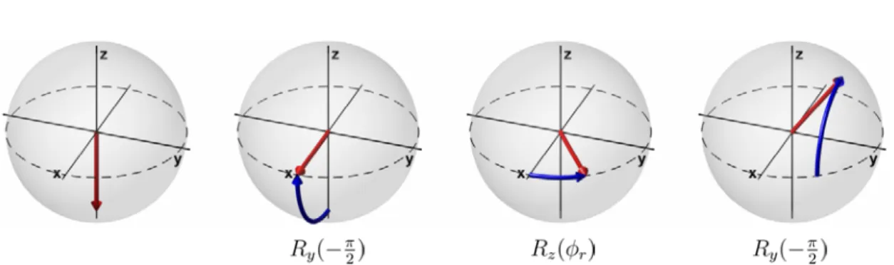
Experimentally, rotations around the z-axis will be usually phase shifts on the LO or a detuning between the LO frequency and the frequency of the atomic transition during an interrogation time. Rotations around x- and y-axis will be implemented by sending a coherent microwave pulse on resonance with an atomic transition onto the atoms. The rotation axis and direction can be set by changing the phase of the LO in steps of π2.
The rotation operators alone are sufficient to describe the evolution of CSSs in an atomic interferometer. Nevertheless, for a highly entangled input state it is more difficult to know the distribution of the state in the Dicke state basis after a rotation from Equation (1.23). The way to solve this problem is based on the work of E. Wigner on the algebra of angular momentum states [Wigner 59]. For this purpose, we introduce the rotation operator
R(α, β, γ) = e−iαJze−iβJye−iγJz , (1.24)
in which contrary to before the rotations are around the z-axis, then around the
y-axis, and then again around the z-axis4. With this operator, any rotation on the
Bloch sphere can be performed. From a physical perspective, it is equivalent to
forming any other sequence of rotations with the operators from Equation (1.23). The rotation of a Dicke state can then be written as
R(α, β, γ)|J, m⟩ =∑ m′ ⟨J, m′|R(α, β, γ)|J, m⟩|J, m′⟩ (1.25) =∑ m′ DJm′m(α, β, γ)|J, m′⟩ , (1.26) where DJ
m′m(α, β, γ) is the Wigner-D matrix. It can be decomposed into
DJm′m(α, β, γ) =⟨J, m′|R(α, β, γ)|J, m⟩ = e−im
′α
dJm′m(β)e−imγ , (1.27)
where we used the definition for the (small) Wigner-d matrix elements
dJm′m(β) =⟨J, m′|e−iβJy|J, m⟩ . (1.28)
The key difficulty is to determine the coefficients dJ
m′m(β), which were found by
Wigner [Wigner 59] dJm′m(β) = [(J + m′)!(J− m′)!(J + m)!(J − m)!]1/2 ×∑ s [ (−1)m′−m+s (J + m− s)!s!(m′− m + s)!(J − m′− s)! × ( cosβ 2 )2J +m−m′−2s( sinβ 2 )m′−m+2s] . (1.29)
Equations (1.24) - (1.29) will be used in Chapter4for the Monte-Carlo simulation of the feedback control of a collective spin state.
1.2.4.2. Ramsey Interferometer
We show now that the rotation operators from Equation (1.23) are sufficient to describe both the mean spin direction and the projection noise of a CSS after unitary evolution on the Bloch sphere. As an example, a Ramsey interferometer is treated. Ramsey interferometry will be the basis of many measurements in this thesis, and is one method to operate atomic clocks as it will be presented in Chapter 5. For the development of his “separated oscillatory field method”, N. F. Ramsey received the Nobel prize in physics in 1989.
Figure 1.4.: Operation principle of a Ramsey interferometer. It includes the prepara-tion of a superposiprepara-tion state, a free evoluprepara-tion time T and the mapping of the acquired phase on the z-axis of the Bloch sphere.
The operation principle of a Ramsey interferometer is depicted in Figure 1.4. The interferometer begins with all atoms prepared in the ground state, i.e. |Ψ0⟩ =
|θ = π, ϕ = 0⟩. A first rotation, called a π
2-pulse, prepares the superposition state
θ = π2, ϕ = 0⟩. During a free evolution time T , the spin rotates by an angle ϕr
around the equator of the Bloch sphere which gives the state θ = π2, ϕ = ϕr ⟩
. The goal of the Ramsey interferometer is to measure the phase ϕr, but usually only the population difference can be read out directly. A final π2-pulse therefore maps the phase on the z-axis of the Bloch sphere and gives the final state θ = ϕr, ϕ = π2
⟩ . The complete interferometer sequence can be described by the unitary evolution operator UR= ei π 2Jye−iϕrJzei π 2Jy . (1.30)
We are interested in the expectation value and the noise of the final measurement along the z-axis. For the expectation value, we have
⟨Jz⟩ = ⟨ Ψ0 UR†JzUR Ψ0 ⟩ (1.31) =− cos ϕr⟨Jz⟩0 + sin ϕr⟨Jy⟩0 (1.32) = J cos ϕr , (1.33)
and for the noise variance (∆Jz) 2 = (∆Jz) 2 0cos 2 ϕr+ (∆Jy) 2 0sin 2 ϕr− sin ϕrcos ϕr⟨JzJy+ JyJz⟩ (1.34) = J 2 sin 2ϕ r . (1.35)
noise, and from error propagation one obtains ∆ϕ = ∆Jz ∂⟨Jz⟩ ∂ϕ = 1 √ Nat . (1.36)
The read out noise for a CSS is therefore independent of the rotation angle. However, this is only true as long as there is no additional detection noise which would be added to the variance in Equation (1.35). The precision of the phase estimation decreases then with the distance from the equator of the Bloch sphere. In many interferometry schemes the phase ϕr is typically small, and it is therefore beneficial to perform the last π2-pulse not around the y- but the
x-axis. The expectation value is then ⟨Jz⟩ = J sin ϕr and the projection noise
∆Jz = √ J 2 cos 2ϕ r.
The same calculations can be repeated with entangled input states, where the ex-pectation values and projection noise can be obtained with the help of the Wigner-D matrix introduced before. The unitary rotations from Equation (1.23) maintain the shape of Gaussian states. A particular problem for a SSS is that if after the interferometer operation the state is close to the poles of the Bloch sphere, the noise of a SSS is even larger than that of a CSS. In this case, the entangled state performs worse in the phase measurement than the uncorrelated state. A solution for this problem based on feedback control with weak measurements was proposed in [Borregaard 13b] and is discussed at the end of Chapter 4.
1.3. Generalized Quantum Measurements
1.3.1. Motivation
Without any specification, the term measurement in quantum mechanics usually refers to an ideal projective measurement. Here, one starts with a quantum system about which some a priori information may or may not be available, and one determines a property by a precise measurement. Since the quantum system possesses with certainty the measured property after the measurement, the a
posteriori quantum state is then in a state both in conformity with the a priori
knowledge and the measurement result. If the quantum state is measured again, the same measurement result will be obtained.
Figure 1.5.: A simple which-path experiment. A single photon is in a superposition of two paths after a beamsplitter (BS). The measurement of the path of the photon by the two photodiodes PD1 and PD2 is not an ideal projective measurement because the photon is destroyed after the measurement and the photodiodes have a technical detection noise.
Although the above way is the standard procedure to define a measurement in quantum mechanics (its mathematical formulation is given below), this situation is never encountered in practice. As an example, consider the which-path experiment depicted in Figure 1.5. A single photons is prepared in a superposition of two paths with two photodiodes PD1 and PD2 for the detection. The photodiodes are connected to a counter and if in one of the two paths there is a “click” we could deduce that a photon arrived. However, the photon has been destroyed by the interaction with the photodiode, and it cannot be measured again. In addition, a photodiode is usually not a perfect detector, and has for example a quantum efficiency (the ratio of the generated charge carriers to photons) below one, and dark counts by thermally generated carriers. Even if a “click” is registered on one of the two counters, it cannot be ascertained that a photon has arrived. Also without the destruction of the photon, the photodetection is therefore not an ideal measurement.
A general way to describe a measurement has to take into account both the possible destructivity by the measurement and uncertainties in the state determi-nation. Here, we will focus on the uncertainty in the state determination, because we treat later the destructivity for our collective spin systems phenomenologically. The understanding of general quantum measurements of collective spins will be the basis for the measurement based feedback control used in this thesis.
As before, a language close to the Kopenhagen interpretation of quantum me-chanics is chosen, although phrases such as “collapse of the wavefunction” are omitted. This does not reflect a bias towards any interpretation, but is merely a practical choice to use formulations with which most physicists are comfortable with. In any case, it should be noted that with strong evidence quantum mechan-ics is a complete theory [Bell 64, Aspect 82, Weihs 98,Rowe 01], and that formal descriptions can be used without reference to any additional interpretation.
1.3.2. Ideal Projective Measurement
We recall at first the concept of an ideal projective measurements on a pure quan-tum state. It is characterized by so called projectors,
Pm =|m⟩ ⟨m| , (1.37)
where m is a measurement result and the vectors{|m⟩} span a basis of the Hilbert space of interest. The projector Pm can be applied to a quantum state |Ψin⟩ to give |Ψout⟩ = Pm|Ψin⟩ √ ⟨Ψin|Pm| Ψin⟩ (1.38) = cm |cm| |m⟩ , (1.39)
where we have used the relation |Ψin⟩ = ∑
mcm|m⟩ in the final equality. The
coefficients c′ms are the probability amplitudes of |Ψin⟩ in the basis {|m⟩}. In the limit where the basis becomes a continuous set, the coefficients c′ms correspond to
the wavefunction of the state. The probability to obtain a measurement result m is p(m) = ⟨Ψin|Pm| Ψin⟩ (1.40) =|⟨m|Ψin⟩|2 (1.41) =|cm| 2 . (1.42)
This equation is also known as the Born rule, named after M. Born who obtained for its statistical interpretation of the wave-function the Physics Nobel prize in
1957. The expectation or average value for the measurement results m is then E(m) =∑ m mp(m) (1.43) =∑ m m⟨Ψin|Pm| Ψin⟩ (1.44) ≡ ⟨Ψin|Om| Ψin⟩ , (1.45) where the definition of the observable for the physical property measured was used:
Om =
∑
m
mPm . (1.46)
In the definitions above, no conditions for the measurement process are needed, except that a measurement result m is obtained using an ideal measurement appa-ratus. We are ready to see now how the model of an ideal projective measurement can be extended to the case where the measurement is not performed with a projec-tor as in Equation (1.39), but with a measurement which contains some uncertainty in the measurement result.
1.3.3. Generalized Measurement Operators
1.3.3.1. Definition
A general quantum measurement is defined by the general measurement operators
Mm, where m is a measurement result. The state after the measurement is
|Ψout⟩ =
Mm|Ψin⟩
√⟨
Ψin Mm†Mm Ψin
⟩ , (1.47)
and the probability to measure m
p(m) = ⟨Ψin Mm†Mm Ψin
⟩
The probabilities should all sum to unity, i.e. 1 =∑ m p(m) (1.49) =∑ m ⟨ Ψin Mm†Mm Ψin ⟩ , (1.50)
which is equivalent to require ∑
m
Mm†Mm = I , (1.51)
where I denotes the identity operator.
1.3.3.2. Example
Consider a two level system prepared in the input state
|Ψin⟩ =
1
√
2(|0⟩ + |1⟩) . (1.52)
We consider the two measurement operators
M0 =√p|0⟩ ⟨0| + √ 1− p |1⟩ ⟨1| , (1.53) M1 = √ 1− p |0⟩ ⟨0| +√p|1⟩ ⟨1| . (1.54)
The operator M0 (M1) is applied when the measurement result m = 0 (m = 1) is obtained. The form of the measurement operators reflects a situation where a measurement result m is obtained but the measurement system has an intrinsic uncertainty. The factor 1−p then corresponds to the probability of a measurement error. The measurement operators fulfill the completeness condition M0†M0 + M1†M1 = I. The state after a measurement result m = 0 is
|Ψout⟩ = M0|Ψin⟩ √⟨ Ψin M0†M0 Ψin ⟩ (1.55) =√p|0⟩ +√1− p |1⟩ . (1.56)
The state is therefore partially projected by the partial information from the mea-surement. In an interesting scenario, another measurement on the state is
per-formed and the result is m = 1. The output state is then |Ψ′ out⟩ = M1|Ψout⟩ √⟨ Ψout M1†M1 Ψout ⟩ (1.57) = √1 2(|0⟩ + |1⟩) , (1.58)
which is same as the input state |Ψin⟩. The presented case where performing a measurement can remove the partial projection of a state is known under the name “weak measurement reversal” (see e.g. [Ueda 92, Katz 08]).
1.3.3.3. Relation to Bayes Theorem
Note that the probability amplitudes are very similarly treated in a general quan-tum measurement as one would update the probability of a classical system. In fact, the principle is the same, only that in one case the information about proba-bilities and in the other case about probability amplitudes is updated. It appears natural for the estimation of a parameter to take the probabilities from the a
pri-ori knowledge of a system, and multiply them with the probabilities from a new
estimate. Normalization gives then the a posteriori probability distribution. This is common practice for the determination of errors and can be formalized writing
p(x, y) = p(x|y)p(y) = p(y|x)p(x), (1.59)
where p(x, y) is the joint probability to have both x and y and p(x|y) and p(y|x) are conditional probabilities. A simple rearrangement of Equation (1.59) leads to Bayes theorem p(x|y) = p(y|x)p(x) p(y) , (1.60) where p(y) = ∫ ∞ −∞ p(y|x)p(x)dx . (1.61)
Bayes theorem tells how the state of knowledge of the variable x, represented by the probability distribution p(x) is updated. A measurement gives new data y, and in order to change our knowledge about x, we have to know how y is related to x. This relationship is usually known in practice. If for example x is a position and y is the measured position with a Gaussian uncertainty, then p(y|x) is peaked at x and has a Gaussian shape. Inserting this in Equation (1.60) gives then the
a posteriori knowledge of x. The general measurement law in Equation (1.47) is therefore nothing else than the Bayes theorem applied to state vectors with probability amplitudes. An ideal projective measurement is analogous to the case where p(y|x) is a delta function.
1.3.3.4. Extension to Density Operators
State vectors are intrinsically probabilistic in nature because they can be expressed as superposition of quantum states with different probability amplitudes. There exists, however, the possibility that for a quantum system there are only informa-tion available about its classical probabilities to be in a certain state5. We assume that we have an ensemble of states|Ψk⟩, which were prepared with different
prob-abilities pk, with
∑
kpk = 1. For each state the conditional probability to measure
a result m is p(m|k) =⟨Ψk Mm†Mm Ψk ⟩ (1.62) =∑ k ⟨ k Mm†Mm Ψk ⟩ ⟨Ψk|k⟩ (1.63) = tr(Mm†Mm|Ψk⟩ ⟨Ψk| ) , (1.64)
where we have used the definition for a trace. The total probability p(m) is
p(m) = ∑ k p(m|k)pk (1.65) =∑ k pktr ( Mm†Mm|Ψk⟩ ⟨Ψk| ) (1.66) = tr(Mm†Mmρ ) , (1.67)
where the density operator ρ is introduced
ρ =∑
k
pk|Ψk⟩ ⟨Ψk| . (1.68)
Even though the density operator is an operator in its nature, it contains all information available about a quantum system. A general measurement can be treated as if the measurement operator acts on each state |Ψk⟩ singularly, and we
5The distinction between probability amplitudes and probabilities is clear in a mathematical formulation, but harder to express in words. In general, the two can be distinguished by the property that probability amplitudes can lead to interference.
can therefore write ρout = ∑ k p(k|m) Mm|Ψk⟩ ⟨Ψk| M † m ⟨ Ψk Mm†Mm Ψk ⟩ (1.69) =∑ k MmρinMm† tr ( Mm†Mmρ ) , (1.70)
where Equation (1.64) and Equation (1.59) were used. The operators in Mm could
be in principle replaced by any other set of operators satisfying the completeness relation (and so the conservation of the total probability). The measurement operators are therefore only a special case of a more general class of operators, called Kraus operators [Kraus 71, Kraus 83]. A map from one density operator to another one is then called a quantum channel which gives a general mean to describe any evolution of a quantum system. A unitary evolution is also a special case of such an evolution, with
ρout = U ρinU†. (1.71)
In the case of a general quantum measurement, it is possible that not the full form of the Kraus operators Mmis known, but only the probabilities of the measurement
results. This is expressed by the operators Em = Mm†Mm, which are non-negative
and Hermitian, and form a so called positive-operator valued measure (POVM). To each probability operator Em of the POVM several different measurement
op-erators Mm and therefore output states can correspond. With the probability
operators, a quantum measurement can be expressed without the knowledge of the all details of the measurement process.
1.3.3.5. General Quantum Measurements of Collective Spin States
Our target is to measure the population difference of a CSS along the z-axis of the Bloch sphere, which is the observable variable in atom interferometry. In the limit
of J ≫ 1, we have shown that the state in the Dicke basis is given by
|Ψin⟩ = |θ, ϕ⟩ =
J
∑
m=−J
with cm = 1 √√ πJ sin θ e−(m2J sin2 θ−J cos θ)2 . (1.73)
The projector in this basis is
Jz =|J, m⟩ ⟨J, m| . (1.74)
We assume that the measurements are nondestructive, i.e. the system remains in a pure state after the measurement. Furthermore, we assume that the measurement has a Gaussian uncertainty with a value σdet with respect to the full spin length J . The situation is then similar to measuring the position on a ruler with a bad
vision. From the probability distribution of the measurement itself, we know the form of Mm†Mm, and taking the square root for the probability amplitudes leads
to Mm = ( 2πσdet2 )−1/4e− 1 4σ2 det (Jz−m)2 . (1.75)
When the measurement operator is applied on the CSS from Equation (1.72), one obtains the output state
|Ψout⟩ = M√m0|Ψin⟩ p(m0) (1.76) =(2πξ2J sin2θ)−1/4 J ∑ m=−J e− (m−µ0)2 2ξ2J sin2 θe−i(J+m)ϕ|J, m⟩ . (1.77)
The index m0 in Equation (1.77) was introduced to distinguish a specific measure-ment result from the variable m for the state vectors. The other variables are the squared squeezing factor
ξ2 = 1
1 + κ2sin2θ , (1.78)
the squared measurement strength
κ2 = σ 2 J σ2 det (1.79) = J 4σ2 det , (1.80)
and the peak position of the Gaussian distribution after the measurement
µ0 =
κ2sin2θm0+ J cos θ
1 + κ2sin2 . (1.81)
The probability of a measurement result m0 is
p (m0) = ⟨θ, φ| Mm†0Mm0|θ, φ⟩ (1.82) = √1 2π ξθ σdet exp [ −ξθ2(m0− J cos θ)2 2σ2 det ] . (1.83)
The definition for the measurement strength is related to the situation when a CSS is prepared on the equator of the Bloch sphere. In this case, the state after the measurement is |Ψout⟩ = ( 2π 1 1 + κ2J )−1/4 ∑J m=−J e− ( m− κ1+κ22 m0 )2 2 1 1+κ2J e−i(J+m)ϕ|J, m⟩ . (1.84)
The measurement strength κ is the ratio of the size of the initial Gaussian wavefunction for a CSS on the equator of the Bloch sphere to the uncertainty of the measurement. The squeezing factor ξ is the ratio of the sizes of the new and the old wavefunction. With an increasing precision of the measurement, the measurement strength increases and the quantum noise of the output state in the measured direction is reduced.
The measurement process can be nicely illustrated by considering only the ab-solute value of the wavefunction as depicted in Figure1.6. The wavefunction after the measurement is simply the initial wavefunction multiplied with another func-tion defined by the measurement operator Equafunc-tion (1.75). It seems reasonable to call this function “measurement function” in analogy to the term wavefunction6. At every position m one then has to multiply the probability amplitudes of the wavefunction and the measurement function. Finally, one normalizes the result by requiring that the total probability of the output wavefunction is equal to 1. In the same spirit, the probability distribution of the measurement results is the
6We only became later aware of the already existing formalism for generalized quantum mea-surements, and derived the above results without this knowledge. The term “measurement function” was very useful in the discussions with the team members, and it is proposed here to keep it for the future.
m A mplit ude m A mplit ude
Figure 1.6.: Illustration of a general quantum measurement with Gaussian variables. The wavefunction Ψoutafter the measurement is simply the multiplication of the initial wavefunction Ψin and the measurement function Mm (with
a final normalization).
squared convolution of the measurement function and wavefunction.
The situation where a CSS is prepared on the equator of the Bloch sphere and undergoes a partial projection is the basic procedure to generate a spin-squeezed state by a nondestructive measurement. The Wineland criterion (Section 1.2.3) is then given by ξS2 = 2J (∆J⊥) 2 |⟨J⟩|2 = ξ2J2 |⟨J⟩|2 = ξ2 η2 coh , (1.85)
where ηcoh = |⟨J⟩|J accounts for the possible decoherence during the measurement process. Another property is that from Equation (1.84) the expectation value for a next measurement is ϵm0 = κ
2
1+κ2m0. The variable ϵ is therefore the corre-lation coefficient between two successive measurements on the same axis on a CSS. Partial projective measurements are an interesting tool to prepare entangled states for metrology. Nevertheless, we take in this manuscript a different path and explore the active control of quantum states in atomic interferometers. The projectivity of the quantum measurements can in this case be a disadvantage. For example, consider the case of an ideal projective measurement. It prepares a Dicke
Figure 1.7.: Weak measurement of a collective spin. Although the uncertainty of the measurement is larger than the projection noise, still the mean spin direction can be determined. If the measurement is nondestructive the spin state is preserved.
state, which has no mean spin direction and can therefore not be read out with the standard Ramsey scheme introduced before. Furthermore, the projectivity of the measurements is in practice linked to their destructivity. In our experiment this will be the case with the number of photons in the optical beam to probe the atoms. To both reduce the projectivity and the destructivity, we can choose the parameter range
1
2J < κ
2 ≪ 1 , ξ ≈ 1 , ϵ≈ 0 . (1.86)
The situation is illustrated in Figure 1.7: even though the uncertainty of the measurement is much larger than the size of the atomic projection noise, it is still possible to obtain information about the population difference. The state after the measurement is
|Ψout⟩ ≈ |Ψin⟩ . (1.87)
Collective quantum states such as a CSS therefore have the interesting property that valuable information about them can be obtained while the state remains basically unchanged. We can therefore obtain information with almost no cost, unlike in most other situations with quantum systems. The precision to which a population difference can be measured goes as σdet
We call such measurements where the uncertainty of the measurement is larger than the uncertainty of the state “weak measurements”. This term has been introduced in connection to schemes where at first one performs on a quantum system a weak (almost non-projective) measurement, and subsequently a strong projective measurement [Aharonov 88]. When the results are postselected accord-ing to the results of the strong final measurements, unexpected predictions about the results of the weak measurements can be made7. In particular, one comes to the non-intuitive result that the weak intermediate measurement could find a spin which is systematically larger then the length of the real spin (see [Aharonov 10] for a good explanation of this effect). Such “weak value amplification” schemes have been used for the measurement of tiny physical effects [Hosten 08,Dixon 09]. Nevertheless, the question of whether weak value amplification can lead to a gain in metrology is still open [Knee 13, Jordan 13, Ferrie 13]. In Appendix A an example for weak measurements with postselection is given.
Weak measurements in the sense of Equation (1.86) will be a central tool in this manuscript. They will be used in combination with feedback control to protect collective spin states against a typical form of decoherence in atomic interferome-ters. On this basis, we develop and demonstrate a feedback protocol to increase the interrogation time in atomic interferometers.
1.3.3.6. Relation to Quantum Non-Demolition Measurements
It should be noted that in the discussion in this chapter, no assumptions on the measurement process itself were made. We have seen that such assumptions are not required, and any quantum measurement can be completely described by the information gain and the general measurement operators Mm. However, there is
the question of how a nondestructive measurement can be performed in practice. The strategy is usually to use an indirect measurement. Here, an auxilary “meter” quantum system interacts and is entangled with the “signal” quantum system. The meter can then be destroyed and its information content treated with a classical apparatus. Because the meter and the signal were entangled by the interaction, the signal quantum system is then fully or partially projected. Such kind of measurement schemes were at first devised by J. von Neumann [von Neumann 96], and conditions for quantum non-demolition (QND) measurements were given
7In the community of quantum optics, the term “weak measurement” is often used equivalently for the case of a weak measurement with postselection, which leads to semantic problems. To make the distinction, it could be better to call the latter “weak value measurement”.
in [Braginsky 80]. In [Grangier 98], criteria to evaluate the quality of the QND measurements are given.
We assume that the total Hamiltonian of the system is H = HS+ HM + HM S,
where HS is the Hamiltonian of the system, HM is the Hamiltonian of the
me-ter and HM S is the interaction Hamiltonian between the system and the meter.
Furthermore, we call the observables of the system and of the meter AS and AM,
respectively. We have then the following three requirements for a QND measure-ment. At first, the meter has to interact with the quantum system,
[HM S, AM]̸= 0 , (1.88)
the interaction between the meter and the signal should not change the signal,
[HM S, AS] = 0 , (1.89)
and the observable should be conserved under free evolution,
[HS, AS] = 0 . (1.90)
In practice, the first and last condition are easily fulfilled, whereas the second condition is problematic. It implies that the meter should not cause any decoher-ence on the signal at all. Experiments with close to no destructivity and variable measurement strength were so far performed on photons in a microwave cavity [Guerlin 07] and on superconducting qubits [Hatridge 13].
Nondestructive measurements on the internal state of atoms are usually per-formed by the dispersive probing with off-resonant light on an atomic transi-tion. There is always a contribution from spontaneous emission and the condi-tion [HM S, AS] = 0 can therefore not be strictly fulfilled. However, within the
scientific community, it has become common practice to take the Wineland cri-terion as a benchmark for a QND measurement on collective spin states. If a CSS can be squeezed according to the Wineland criterion, then the nondestructive measurement can be called a quantum non-demolition measurement. Since in our experimental setup we cannot fulfill the Wineland criterion, we use in the following chapters the term nondestructive measurements to describe our detection system.
2.1. Introduction
In this chapter, our procedure to prepare a large coherent ensemble of two-level atoms is described. Coherence can refer for an atomic cloud to the internal states, the external states, or both. In atomic clocks, mainly the internal state purity is of interest. In a matter-wave Bragg interferometer, only the external states are manipulated, and therefore an atomic sample should be as cold as possible and preferably be without atomic interactions. In a Raman interferometer, both the internal and external states are equally crucial. Nevertheless, since in most interferometers the internal and external states of the atoms can couple to each other, we aim to achieve at the same time a high purity both of the internal and external states.
In its initial orientation, our experimental setup was designed as a compact prototype for matter-wave experiments, combined with a nondestructive detec-tion system for the atoms. We work with the atomic species 87Rb, which is routinely used for cold atom experiments in laboratories around the world, and for which first companies sell dedicated products1. The focus in this chapter is therefore on the non-standard experimental solutions we have chosen for our setup. A unique feature in our experimental setup is an optical cavity with mirrors arranged in a butterfly configuration, presented in Section 2.3. The optical cavity stores and therefore enhances the field derived from a telecom laser at 1560 nm. The light in the cavity is used as an optical trap for the atoms, and because of the power enhancement of the cavity less laser power is needed for the same depth of the trap. A detailed description of the vacuum system for the atoms, the magneto-optical trap and the optical cavity was already given in the PhD thesis of Simon Bernon [Bernon 11a], and I will therefore only highlight the
1One company, Quantel, used our setup to test one of their laser systems especially designed for the cooling of 87Rb. Another company, ColdQuanta, sells even an entire setup for the production of cold atomic clouds.
main characteristics here (Section 2.2 and Section 2.3). To use the the optical cavity, the frequency of the dipole trap laser has to be kept on resonance with the cavity via a feedback system. We developed a new method for such a stabi-lization system based on serrodyne frequency shifting as described in Section 2.3.4. One of our first goals with the experimental setup was to obtain a Bose-Einstein condensate with the help of the cavity-enhanced light field, and our results are shown in Sections 2.4 and 2.5. For our experiments with the nondestructive detection system we were only interested in the internal states of the atoms. Because of their higher atom number we therefore chose to continue our work with trapped thermal clouds with a temperature of around 10 µK.
The optical dipole trap at 1560 nm causes a large light shift on the optical transitions used to probe the atoms. In Section 2.6, we describe a compensation method which cancels this large light shift with an auxiliary laser at 1529 nm. This allows us to treat the optical transitions of 87Rb as if the atoms would be probed in free space. Since we worked with a very dense atomic cloud, multiple scattering of light did not allow us to use a conventional technique for the preparation of the internal atomic states. In the last part of this chapter (Section 2.6.2), we show how we dealt with this problem and describe our state preparation method. The trapped atomic ensembles with no differential light shift on the optical transitions are then the basis for the work in the succeeding chapters.
2.2. Vacuum System and Magneto-Optical Trap
Cold atoms must me hold in ultra high vacuum to avoid their random interaction with the environment. This prevents heating of the atoms or random changes of their internal atomic states. To obtain a cold atomic cloud with a high atom number and a long lifetime, we use the vacuum system shown in Figure 2.1. It consists of two chambers, one to cool atoms from the background pressure of a solid sample of87Rb, and one for the storage of the atoms in ultra high vacuum.
The first vacuum chamber contains a two dimensional magneto-optical trap (2D MOT) and the second chamber a three dimensional magneto-optical trap (3D MOT) and a dipole trap enhanced by an optical cavity. In the second chamber the experiments are performed and it is called the science chamber. The pressure in the 2D MOT chamber is below 10−7 mbar and in the science chamber below