HAL Id: tel-01113856
https://pastel.archives-ouvertes.fr/tel-01113856
Submitted on 6 Feb 2015
HAL is a multi-disciplinary open access archive for the deposit and dissemination of sci-entific research documents, whether they are pub-lished or not. The documents may come from teaching and research institutions in France or abroad, or from public or private research centers.
L’archive ouverte pluridisciplinaire HAL, est destinée au dépôt et à la diffusion de documents scientifiques de niveau recherche, publiés ou non, émanant des établissements d’enseignement et de recherche français ou étrangers, des laboratoires publics ou privés.
simulation of aeronautical propulsion systems
Nadezda Petrova
To cite this version:
Nadezda Petrova. Turbulence-chemistry interaction models for numerical simulation of aeronautical propulsion systems. Modeling and Simulation. Ecole polytechnique X, 2015. English. �tel-01113856�
DOCTOR OF THE ECOLE POLYTECHNIQUE
Specialization: Applied Mathematics
by
Nadezda PETROVA
Turbulence-chemistry interaction models for numerical simulation
of aeronautical propulsion systems
Defended on 16 January 2015 in front of the jury:
Dr. Arnaud MURA
ISAE-ENSMA
Referee
Dr. Serge SIMO¨
ENS
LMFA, ´
Ecole Centrale de Lyon
Referee
Prof. Gregoire ALLAIRE
CMAP, ´
Ecole Polytechnique
Examiner
Dr. Nicolas BERTIER
ONERA/DEFA
Examiner
Dr. Pascal BRUEL
LMA, Universit´
e de Pau
Examiner
Prof. Andrei LIPATNIKOV
Chalmers, Sweden
Examiner
Dr. Olivier SOULARD
CEA/DAM
Examiner
Prof. Vladimir SABELNIKOV
ONERA/DEFA
Supervisor
Acknowledgments
I wish to express my sincere gratitude to my thesis director Vladimir Sabelnikov for the honor he gave me by accepting my candidacy for the present work, sharing his expert knowledge of the combustion models and comprehensive guidance during my PhD project.
I express my special thanks to Nicolas Bertier for his invitation to participate in FTC project in a difficult situation where we had not yet obtained significant advances on the original Monte-Carlo topic, and for his subsequent help with the architecture of CEDRE code.
I remain indebted to Olivier Soulard for his great idea for solving SPDEs. I would like to thank him and Roland Duclous for the opportunity to take part in turbulence modeling project during CIRM summer school.
I would like to thank a lot Arnaud Mura and Serge Simoens, for accepting to take part in the jury as referees, and for their detailed and insightful reviews of my manuscript. Many thanks to Gregoire Allaire, Pascal Bruel, Andrei Lipatnikov for the careful examination of the present work. I would like to thank all the members of the jury for hard and interesting questions, resulted in a fruitful in-depth discussion following the defense.
I am very thankful to Philippe Grenard, Lionel Matuszewski, Thomas Le Pichon, Dmitry Davidenko, Aymeric Boucher and Yann Moule, and all the DEFA team for their readiness to help and professionalism. I would like to thank all my colleagues for all they gave me during these three years.
Abstract
Modeling the turbulence-chemistry interaction is a key point in the numerical sim-ulation of the combustion in the air-breathing engines. The present work is devoted to adaptation and integration of the different turbulent combustion models into the ONERA industrial code CFD package for diphasic reactive flows (CEDRE). The first part of the thesis is focused on the quasi-linear hyperbolic stochastic partial differential equations (SPDEs) which are statistically equivalent to a transport equation for the joint velocity-scalars probability density function (PDF). It is shown that in order to preserve the equivalence between the SPDEs and the transport equation for the joint velocity-scalars PDF, multivalued solutions of the SPDEs should be taken into account. A new stochastic method to solve the SPDEs, recently proposed by O. Soulard [Emako-Letizia2014], is considered and validated on one-dimensional test-cases. It is shown that this method is able to recover the multivalued solutions of the SPDEs in the statistical sense.
The numerical solution of the SPDEs is time consuming, therefore the second part of the thesis is concerned with a flamelet tabulated chemistry (FTC) and an extended partially stirred reactor (EPaSR) models. In the framework of CEDRE CFD software the FTC approach is updated, presuming that the distribution is given by a 𝛽-PDF. The adaptation of the LES/EPaSR model [SabelnikovFureby2013] to the RANS and its integration into CEDRE are done. The EPaSR and the FTC with the presumed 𝛽-PDF are validated against experimental data [MagreMoreau1988] on a configuration of a backward-facing step combustor. It is shown that the RANS/EPaSR calculation yields the best agreement with the experiment compared to other considered approaches.
Keywords: stochastic partial differential equations, probability density function, multivalued solution, extended partially stirred reactor, flamelet tabulated chemistry model
R´esum´e
La mod´elisation de l’interaction turbulence-chimie est un point cl´e dans la si-mulation num´erique des ´ecoulements r´eactifs turbulents. Cette th`ese est consacr´ee `a l’adaptation et l’int´egration de diff´erents mod`eles de combustion turbulente dans le code d’´ecoulements diphasiques r´eactifs pour l’´energ´etique (CEDRE) de l’ONERA. La premi`ere partie de la th`ese est d´edi´ee `a l’´etude des ´equations quasi-lin´eaires hy-perboliques stochastiques aux d´eriv´ees partielles (SPDEs) qui sont statistiquement ´
equivalentes `a une ´equation de transport pour la fonction de densit´e de probabilit´e (PDF) jointe vitesse-scalaires. Il est d´emontr´e que pour pr´eserver l’´equivalence entre les SPDEs et l’´equation de transport pour la PDF jointe vitesse-scalaires, les solutions mul-tivalu´ees des SPDEs doivent ˆetre prises en compte. Une nouvelle m´ethode stochastique pour r´esoudre les SPDEs, r´ecemment propos´ee par O. Soulard [EmakoLetizia2014], est ´
etudi´ee et valid´ee sur des cas-tests unidimensionnels. Il est montr´e que cette m´ethode permet de trouver les solutions multivalu´ees des SPDEs au sens statistique.
La r´esolution num´erique des SPDEs ´etant particuli`erement coˆuteuse, une seconde voie a ´et´e explor´ee au cours de cette th`ese. Il s’agit, dans la deuxi`eme partie de ce m´emoire, de la mise en œuvre du mod`ele ”flammelettes tabul´ees pour la chimie” (FTC) et du mod`ele ”r´eacteur partiellement m´elang´e ´etendu” (EPaSR). Avec le code CEDRE, l’approche des FTC est mise `a jour en supposant une distribution de type 𝛽-PDF. L’adaptation LES/EPaSR [SabelnikovFureby2013] pour le RANS et son int´egration dans CEDRE ont ´et´e r´ealis´ees. Les mod`eles EPaSR et ”FTC avec 𝛽-PDF pr´esum´ee” ont ´et´e valid´es par rapport aux donn´ees exp´erimentales [MagreMoreau1988] sur une configuration de flamme stabilis´ee par une marche descendante. Il est montr´e que le calcul RANS/EPaSR donne un meilleur accord avec l’exp´erience que les autres ap-proches ´evalu´ees.
Mots cl´es : ´equations aux d´eriv´ees partielles stochastiques, fonction de densit´e de probabilit´e, solutions multivalu´ees, r´eacteur partiellement m´elang´e ´etendu, flammelettes tabul´ees pour la chimie
Contents 7
List of symbols 11
List of dimensionless numbers 14
List of abbreviations 15
1 Introduction 19
2 Background 23
2.1 Turbulence characteristics 24
2.1.1 Homogeneous isotropic turbulence 25
The Kolmogorov hypothesis 28
2.2 Flame structure 28
2.2.1 Premixed flame 28
Regimes in premixed combustion 29
2.2.2 Non-premixed flame 32
2.3 Navier-Stokes equations for aerothermochemistry 34
2.3.1 Conservation of mass and species 34
2.3.2 Chemical kinetics 35
2.3.3 Conservation of momentum 35
2.3.4 Conservation of total energy 36
2.3.5 State law of an ideal gas 36
2.4 Reynolds averaged Navier-Stokes (RANS) approach 37
2.4.1 Definition of the ensemble average 37
2.4.2 Averaged Navier-Stokes equations 37
2.4.3 Closure of the RANS equations 38
2.4.4 Turbulence models 39
2.5 Large eddy simulation (LES) 40
2.5.1 Closure of the LES equations 40
2.6 General models of turbulent combustion 41
2.6.1 PDF approach 41
Eulerian PDFs 41
Presumed PDF 42
Transported Eulerian PDF 44
2.6.2 Partially stirred reactor models 51
Eddy dissipation concept 51
Partially stirred reactor model 53
Extended partially stirred reactor model 56
Unsteady partially stirred reactor model 58
2.6.3 Thickened flame model 59
I New approach to solve SPDEs statistically equivalent to a
transport equation for velocity PDF
61
3 Eulerian (Field) Monte Carlo methods for solving the Favre one-time
one-point velocity PDF transport equation 63
3.1 Description of the problem 65
3.1.1 One-dimensional model PDF equation 65
3.1.2 One-dimensional SPDEs 68
3.1.3 Equivalence between SPDEs and PDF equation 71
3.2 Stochastic numerical schemes 72
3.2.1 Schemes for partial differential equations 72
Numerical notations for stochastic schemes 74
Numerical stochastic schemes 75
Mean density conservation in stochastic schemes 80
3.2.2 Schemes for stochastic partial differential equations 80
General remarks 82
3.3 Numerical tests 83
3.3.1 Backward step velocity profile 83
Numerical solution 83
3.3.2 Scheme non-dissipativity test 96
PDF 96
PDEs 96
Numerical solution: test 1 97
3.3.3 Statistically homogeneous velocity fluctuations test 106
PDF 106
SPDEs 107
Numerical solution 110
3.3.4 Model PDF equation with non-zero RHS 127
PDF 127
SPDEs 127
Numerical solution 127
3.4 Conclusions 134
II Standard models of turbulent combustion
137
4 Flamelet tabulated chemistry (FTC) model 139
4.1 Original implementation of FTC beta-PDF model in CEDRE 139
4.1.1 Modeling of Favre-averaged progress variable 139
4.1.2 Modeling of Favre variance of progress variable 140
Transport equation 140
Algebraic expression 141
4.1.3 Modeling of Favre-averaged mixture fraction 142
4.1.4 Modeling of Favre variance of mixture fraction 142
Transport equation 142
Algebraic expression 142
4.1.5 Gradient of Favre-averaged progress variable 142
4.1.6 Coupling between tabulated chemistry and CEDRE 142
4.1.7 Presumed beta-PDF 143
4.1.8 Algorithm of beta-PDF integration 143
4.2 Updated FTC beta-PDF model 144
4.2.1 New models for dissipation and source terms 144
4.2.2 Gradient of Favre-averaged progress variable 144
4.2.3 Algorithm of beta-PDF integration 145
4.2.4 Numerical implementation of beta-PDF integration 147
Study of convergence of the semi-analytic beta integration method 148
5 Transported partially stirred reactor (TPaSR) model 151
5.1 Original EPaSR model 151
5.2 TPaSR model: EPaSR adaptation to CEDRE 152
6 Backward-facing step flow 155
6.1 A3C experimental setup 156
6.2 RANS nonreactive backward-facing step flow calculation 157
6.2.1 Computational domain and grid 157
6.2.2 Physical models 158 6.2.3 Boundary conditions 158 6.2.4 Numerical methods 159 6.2.5 Computational strategy 159 6.2.6 Results 162 Recirculation region 162 Favre-averaged velocity 163 RMS velocity fluctuations 165 Turbulent frequency 168 6.2.7 Conclusions 168
6.3 RANS reactive backward-facing step flow calculation 169
6.3.1 Numerical setup 169
6.3.2 Combustion modeling 170
Quasi-laminar approaches 171
PFTC 𝛽-PDF models 178
TPaSR model 186
6.3.4 Conclusions 195
6.4 LES reactive backward-facing step flow calculation 195
6.4.1 Computational domain and grid 195
6.4.2 Physical models 196
6.4.3 Boundary conditions 196
6.4.4 Combustion modeling and numerical schemes 199
6.4.5 Computational strategy 199
6.4.6 Results 200
Mean temperature 200
Recirculation region 202
Mean streamwise velocity 203
Mean transverse velocity 204
Mean mass fractions 207
Velocity fluctuations 210
Impact of reflecting boundary conditions 213
6.4.7 Conclusions 216
6.5 Conclusions 216
7 Conclusions and future work 219
7.1 Conclusions 219
7.2 Future work 220
7.2.1 SPDEs 220
7.2.2 TPaSR model 220
7.2.3 FTC with presumed beta-PDF model 221
A Some aspects of SPDEs modelling 223
A.1 Random choice method (RCM) for solution satisfying entropy increase condition223
A.2 Stochastic Runge-Kutta method 226
A.3 Schemes for SPDEs statistically equivalent to the joint velocity-scalar PDF
equation 227
A.4 𝑛 dimensional space schemes for PDEs 228
A.5 Numerical tests 230
A.5.1 Step velocity profile 231
PDF 231
PDEs 231
Numerical solution 232
A.5.2 Ramp velocity profile 234
PDF 234
PDEs 235
Numerical solution 239
A.5.3 Triangle velocity profile 247
PDEs 248
Numerical solution 251
A.5.4 Hat velocity profile 254
PDEs 254
Numerical solution 254
A.5.5 Scheme non-dissipativity test 259
Numerical solution 259
A.6 Study of Langevin equation 269
B Dependence of solution on computational grid in reactive
backward-facing step flow 273
B.1 Numerical setup 273 B.2 Results 275 B.2.1 RANS/PFTC beta-PDF 275 B.2.2 RANS/TPaSR 281 List of figures 287 List of tables 300 Bibliography 303
𝐴, 𝐵, 𝐸𝑎 Arrhenius law parameters
𝐶𝑓 Friction coefficient
𝐶𝑝 Specific heat capacity at constant pressure of the
mix-ture
J/(kg K)
𝐶𝑠 Smagorinsky model constant
𝐶𝜇 𝑘 − 𝜀 model constant
𝐶𝑝𝑘 Specific heat capacity at constant pressure of species
𝑘
J/(kg K)
𝐶 Progress variable
𝐷𝑘 Diffusion coefficient of species 𝑘 m2/s
𝐹 (𝑄) Fourier transformation of the quantity 𝑄
𝑁𝑏𝑟 Number of different branches of multivalued solution
𝑁𝑟 Number of realizations
𝑁𝑠𝑝 Number of species
𝑃 Pressure Pa
𝑅0 Ideal gas constant J/(mol K)
𝑆𝐿 Laminar flame speed m/s
𝑇 Temperature K
𝑌𝑘 Mass fraction of species 𝑘
𝑍 Mixture fraction
Δ𝑡 Time step s
𝛿𝐿 Laminar flame thickness m
˙
𝜔𝑘 Rate of chemical reaction of species 𝑘 kg/(m3 s)
𝜂𝐾 Kolmogorov length scale m
𝛾𝑒𝑞* Volume fraction of fine structures in equilibrium state
𝛾* Volume fraction of fine structures
𝜆𝑘 Thermal conductivity of species 𝑘 W/(m K)
𝜆 Thermal conductivity of the mixture W/(m K)
𝜇𝑘 Dynamic viscosity of species 𝑘 kg/(m s)
𝜇 Dynamic viscosity of the mixture kg/(m s)
𝜈 Kinematic viscosity m2/s
𝜔 Turbulent frequency Hz
𝜌 Density kg/m3
𝜏* Subgrid residence time scale s
𝜏𝐾 Kolmogorov time scale s
𝜏𝑐ℎ Chemical time scale s
𝑆 Symmetric part of the strain tensor
𝑉 Sample space of velocity m/s
𝑢′′ Favre velocity fluctuations m/s
𝑢′ Reynolds velocity fluctuations m/s
𝑢* Stochastic velocity m/s
𝑢𝑅𝑀 𝑆 RMS velocity fluctuations m/s
𝑢 Velocity vector m/s
𝜀 Turbulence dissipation rate m2/s3
̃︀
𝑄 Favre average of the quantity 𝑄
̃︀ 𝑓 Favre PDF 𝜉 Stochastic noise 𝑒𝑡 Total energy J/kg 𝑓𝛽 𝛽-PDF 𝑔 Fluctuating velocity PDF ℎ𝑡 Total enthalpy J/kg 𝑖𝑟𝑒𝑎 Realization index
𝑘 Kinetic energy of the turbulence J/kg
𝑙 Turbulent length scale m
𝑟* Stochastic density kg/m3
𝐷𝑎 Damkholer number
𝐾𝑎 Karlovitz number
𝑃 𝑟 Prandtl number
𝑅𝑒𝑡 Turbulent Reynolds number
𝑅𝑒 Reynolds number
𝑆𝑐 Schmidt number
𝑐𝑓 𝑙 Courant-Friedrich-Lewy number
BML Bray–Moss–Libby model
BVM Boussinesq viscosity model
CEDRE CFD package for diphasic reactive flows (Code d’´ecoulements
diphasiques r´eactifs pour l’´energ´etique)
CFD computational fluid dynamics
CFL Courant-Friedrich-Lewy condition
DNS direct numerical simulation
EARSM explicit algebraic Reynolds stress model
EBU eddy break-up
EDC eddy dissipation concept
EMC Eulerian Monte Carlo
EPaSR extended partially stirred reactor
FTC flamelet tabulated chemistry model
GForce generalized first order centered method
GLM generalized Langevin model
ITNFS intermittent turbulent net flame stretch
LAERTE Reactive flow and research techniques laboratory (Laboratoire des
ecoulements r´eactifs et de leurs techniques d’etudes)
LES large eddy simulation
LFA laminar flamelet assumption
LHS left-hand side
LMC Lagrangian Monte Carlo
MUSCL monotonic upstream scheme for conservation laws
noTCI chemistry model without turbulence-chemistry interaction
O-U Ornstein-Uhlenbeck
ODE ordinary differential equation
ODFI Riemann invariants-based flow decentering operator (op´erateur de
d´ecentrement sur les flux avec l’utilisation des invariants de Riemann)
PaSR partially stirred reactor
PDE partial differential equation
PDF probability density function
PFTC premixed flamelet tabulated chemistry model
PRECCINSTA prediction and control of combustion instabilities in tubular and
an-nular gas turbine combustion systems
PSR perfectly stirred reactor
QL RCM quasi-laminar model with reduced chemical mechanism
RANS Reynolds-averaged Navier-Stokes equations
RCM random choice method
RHS right-hand side
RK2 explicit second order Runge-Kutta method in time
RMS root mean square
SGF stochastic GForce method
SGod stochastic Godunov method
SL-F stochastic Lax-Friedrichs method
SL-W stochastic Lax-Wendroff method
SODE stochastic ordinary differential equation
SPDE stochastic partial differential equation
TCI turbulence-chemistry interaction
TFLES thickened flame large eddy simulation
TPaSR transported partially stirred reactor
Introduction
The modern energy and environmental context motivate the improvement of combustion systems in air-breathing chambers. The structure of turbulent flames in industrial combus-tion chambers is complex: it is governed by turbulence, two-phase injeccombus-tion, chemical kinetics, acoustics and radiation. Once validated by comparison with experimental data, numerical simulations allow improving the understanding of the different physical mechanisms, in par-ticular, analyzing combustion stability, and explaining formation of polluting emissions. The description of the turbulence-chemistry interaction (TCI) is a key point in the development of such numerical methods. Approaches based on probability density function (PDF) offer compelling advantages for modeling reacting turbulent flows [Pope2000]. They provide an effective resolution to the closure problems that arise from averaging or filtering of the highly nonlinear chemical source terms, from modeling the effects of convection, body forces. There are two different PDF-based methods: the first assumes a certain approximate shape of the PDF (presumed PDF) and the second consists in solving a transport equation for the PDF. Over the past years, the use of the presumed PDFs for combustion progress variable or/and mixture fraction has been gaining popularity as an approach to average reaction rates in premixed and non-premixed turbulent flames. Commonly invoked for this purpose is a 𝛽-PDF, with the parameters determined by the values of its first and second moments. These moments are computed by integrating proper balance equations. The disadvantage of the presumed PDF method is the absence of an universality of the PDF. Therefore the results of each simulation should be validated case by case.
The approach based on the transport equation for the one-time one-point joint velocity-scalars PDF [Pope1985] is a natural and promising tool for the description of the TCI. It is nonetheless counterbalanced by a severe numerical constraint: the joint velocity-scalars PDF possesses a potentially high number of dimensions, which induces heavy computational cost. The finite difference methods cannot be used, as their cost increases exponentially with dimensionality. The common approach to circumvent this difficulty is to use the Monte Carlo methods, which yield a linearly growing effort and therefore are well suited to solve PDF equations.
In the field of turbulent combustion, Lagrangian Monte Carlo (LMC) methods [Pope1985] have become an essential component of the PDF approach. The LMC methods are based on stochastic particles, which evolve from prescribed stochastic ordinary differential equa-tions (SODEs). Numerous publicaequa-tions document the convergence and accuracy of the LMC
methods. However, the development of new Eulerian Monte Carlo (EMC) methods are useful and stimulating, since the competition between the LMC and the EMC methods could push both approaches forward.
The EMC methods are based on stochastic Eulerian fields, which evolve according to the stochastic partial differential equations (SPDEs) statistically equivalent to the PDF
equa-tion. The EMC methods have already been proposed in [Vali˜no1998; SabelnikovSoulard2005;
SabelnikovSoulard2006], in order to compute the one-time one-point PDF of turbulent re-active scalars. The methods discussed in these works are still numerically expensive, since their Courant-Friedrich-Lewy condition (CFL) criterion is similar to an advection/diffusion stability criterion.
Recently O. Soulard and V. Sabelnikov [SoulardSabelnikov2006; SabelnikovSoulard2010] have proposed SPDEs to solve a transport equation for the Favre joint PDF of velocity fields and turbulent reactive scalars. The Ornstein-Uhlenbeck (O-U) process for fluctuating velocity allows using the time step which is proportional to a grid size divided by total stochastic velocity. From this point of view the SPDEs are less expensive and allow more precise determination of PDF statistics.
The first part of the thesis is focused on the developing the EMC methods to solve the transported joint velocity-scalars PDF. They are time consuming therefore the second part of the thesis is concerned with a flamelet tabulated chemistry (FTC) with a presumed 𝛽-PDF and with an extended partially stirred reactor (EPaSR) models. These standard turbulence combustion approaches are less expensive.
The outline of this thesis is as follows. The fundamentals of the turbulence, the premixed and the non-premixed flames are recalled in the chapter 2. Then some background infor-mation on governing equations and various modeling approaches for turbulent combustion is given.
The chapter 3 presents the quasi-linear hyperbolic SPDEs which are statistically equiv-alent to the transport equation for the joint velocity-scalars PDF. It is shown that in order to preserve the equivalence between the SPDEs and the joint velocity-scalars PDF transport equation, the multivalued solutions of the SPDEs should be taken into account. Recently, the level set method [LiuOsher2006] has been developed to capture multivalued solutions of the deterministic hyperbolic PDEs. It should be noted that the level set method augments the problem dimension by one in the physical space, i.e (𝑡, 𝑥) + 1. However, the direct appli-cation of the level set method to the SPDEs needs a further development, because of a strong variation of the number of the branches of multivalued solutions of the SPDEs. Therefore, in the thesis a new stochastic method (proposed by O. Soulard [EmakoLetizia2014]) is applied to solve the SPDEs.
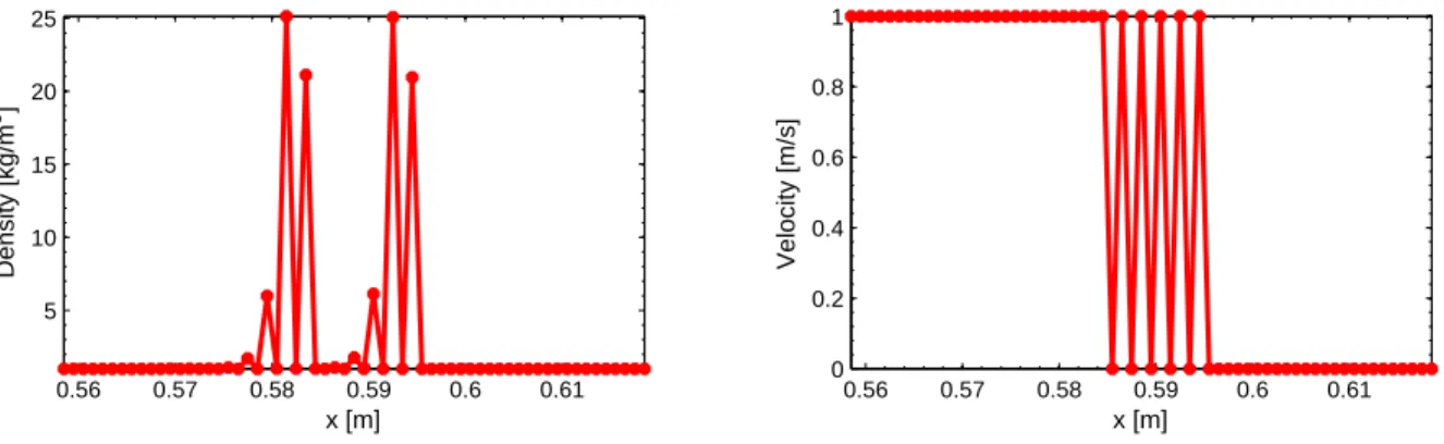
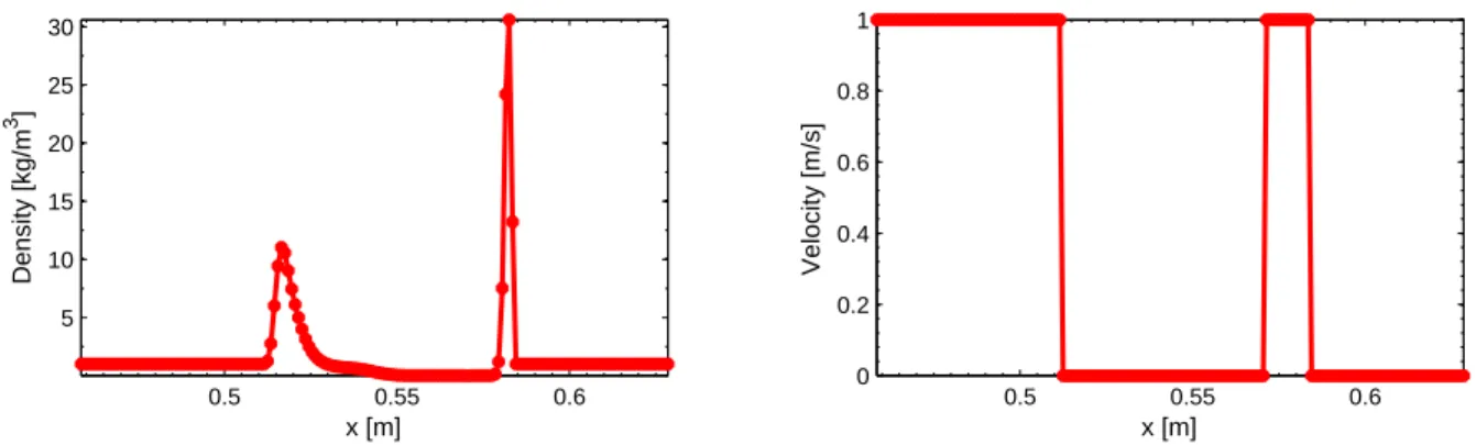
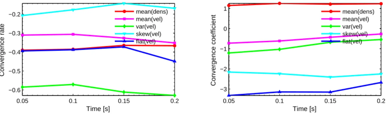
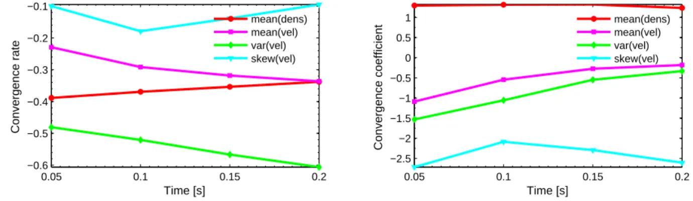
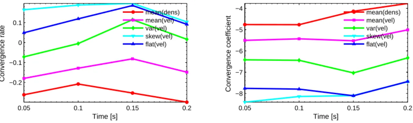
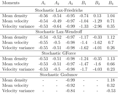
Validation of the new method is carried out on a series of one-dimensional test-cases. It is shown that the method is able to recover multivalued solution in the statistical sense. Velocity moments are compared with the analytical solutions of the PDF equation if they exist or with the numerical solutions of the PDF equation, and a good agreement is found. Numerical accuracy issues, such as spatial and statistical convergence rates, are investigated. A FTC method is updated into the current version of CFD package for diphasic reactive flows (CEDRE) software, presuming that the distribution is given by a 𝛽-PDF. The chapter 4 describes the original algorithm [Savre2010] along with performed improvements. The semi-analytic 𝛽 integration method [LienLiu2009] is extended from one variable (mixture fraction)
to two variables case (mixture fraction variable and progress variable). This modification permits to overcome boundary singularities in integration of the 𝛽-PDF over the mixture fraction and the progress variables.
The chapter 5 describes the adaptation of the large eddy simulation (LES)/EPaSR model [SabelnikovFureby2013] to the Reynolds-averaged Navier-Stokes equations (RANS) and its integration into CEDRE. This model is referred to as the transported partially stirred reactor (TPaSR) model.
RANS and LES simulations of a premixed methane/air flow in a backward-facing step combustor are presented in the chapter 6. The TPaSR, the FTC without TCI and the FTC with a presumed 𝛽-PDF models are considered, and the effects of various modeling assump-tions are discussed. Validation of numerical results on experimental data [MagreMoreau1988] are done. It is demonstrated that the RANS/TPaSR with a 𝑘−𝑙 turbulence model calculation yields the best agreement with the experiment compared to other considered methods.
The conclusions are summarized in the chapter 7 along with suggestions for future work. Some results of the thesis are published in the following communications:
∙ C. Emako, V. Letizia, N. Petrova, R. Sainct, R. Duclous, and O. Soulard. “Diffusion limit of Langevin PDF models in weakly inhomogeneous turbulence”. In: CEMRACS (2014)
∙ N. Petrova and V. Sabelnikov. “Simulation of turbulent combustion in air-breathing chambers: extension of Eulerian Monte Carlo methods”. In: 13th Onera-DLR Aerospace Symposium ODAS (2013)
Background
Turbulent combustion is encountered in most practical combustion systems such as rock-ets, internal combustion or aircraft engines, industrial burners and furnaces; while laminar combustion applications are almost limited to candles, lighters and some domestic furnaces (examples can be found in [PoinsotCandel1995; Pope2000]). Studying and modeling turbu-lent combustion processes is therefore an important issue to develop and improve practical systems (i.e. to increase efficiency and reduce fuel consumption and pollutant formation). As combustion processes are difficult to handle using analytical techniques, numerical com-bustion for turbulent flames is a fast growing area.
There are three main numerical approaches used in turbulent combustion:
∙ Direct numerical simulation (DNS): Direct Numerical Simulation consists in solv-ing the Navier-Stokes equations, resolvsolv-ing all the scales of motion without any turbu-lence model. The flow is described by the instantaneous fields from which all other information is determined. DNS is the simplest and unrivaled in accuracy approach. Yet its cost is extremely high and furthermore it increases very rapidly with Reynolds number. Consequently, today this method is not applicable to the simulation of prac-tical engineering problems, in particular, to high-Reynolds-number flows.
∙ LES: Large Eddy Simulation explicitly computes structures which are larger than the computational mesh size of the flow field whereas the effects of the smallest ones are modeled. LES provide unsteady and spatially-filtered quantities. These instantaneous quantities cannot be directly compared to the experimental flow fields. Only the sta-tistical quantities extracted from LES can be compared with the experimental data. Computationally LES is less expensive than DNS.
∙ RANS: Reynolds averaged Navier-Stokes equations describe mean flow fields and are adapted to practical industrial simulations. In this approach any instantaneous quantity is decomposed into a time or ensemble average and a fluctuating component. Unclosed quantities in the governing equations are modeled, using turbulence and combustion models.
In the present work we limit ourselves to model the turbulent reactive flow within com-putationally accessible RANS and LES approaches.
This chapter is organized as follows. First, we recall energy cascade and the Kolmogorov hypotheses, and introduce various scales of motion. Then the general description of the
flame structure is given. After that we formulate the governing equations describing the fundamental properties of turbulent reacting flows. Finally, we describe some general models of turbulent combustion.
2.1
Turbulence characteristics
Following the description of turbulent flows given in the book of [Peters2000], we mention the main characteristics of turbulent flow (for simplicity, a nonreactive density constant case is considered in this section).
Turbulent flow appears at sufficiently high Reynolds number
𝑅𝑒 = 𝑈 𝐿
𝜈 , (2.1)
where 𝑈 is a characteristic velocity of the flow, 𝐿 is a characteristic length scale of the geometry and 𝜈 is a kinematic viscosity of the fluid. It possesses several characteristic features ∙ Irregularity. Turbulent flow is irregular, random and chaotic, with a large number of
eddies of different length scales.
∙ Diffusivity. In turbulent flow the diffusivity increases.
∙ High Reynolds Numbers. Turbulent flow occurs at high Reynolds number. ∙ Three-Dimensional. Turbulent flow is always three-dimensional.
∙ Dissipation. Turbulent flow is dissipative, which means that there is a steady transfer of kinetic energy from the large scales to the small scales and that this energy is then transformed into the internal energy at the small scales by viscous dissipation. Such the behavior is usually referred to as the eddy cascade hypothesis.
∙ Continuum. Even though we have small turbulent scales in the flow they are much larger than the molecular scale and we can treat the flow as a continuum.
An example of a turbulent jet is shown in fig. 2.1. It enters with a high velocity into initially quiescent surroundings. The large velocity difference between the jet and the sur-roundings generates shear layer instability, which after a transition region, becomes turbulent. In order to characterize the distribution of eddy length scales at any position within the jet, the axial velocity 𝑢 is simultaneously measured at time 𝑡 at points 𝑥 and 𝑥+𝑟, where 𝑟 is
𝑟 = 𝑟𝑒𝑟, 𝑟 is a distance between two spatial points and 𝑒𝑟 is a unit vector in the direction 𝑟.
The correlation between two axial velocities 𝑢(𝑡, 𝑥) and 𝑢(𝑡, 𝑥 + 𝑟) is defined by the average
𝑅(𝑡, 𝑥, 𝑟) = 𝑢′(𝑡, 𝑥)𝑢′(𝑡, 𝑥 + 𝑟), (2.2)
fuel air unstable shear layer transition to turbulence fully developed turbulent jet x x+r
Figure 2.1: Schematic presentation of two-point correlation measurements in a turbulent jet
2.1.1
Homogeneous isotropic turbulence
For homogeneous isotropic turbulence the velocity field is invariant under translations, rota-tions and reflecrota-tions of the coordinate system. For this case the normalized axial correlation is 𝑓 (𝑡, 𝑟) = 𝑅(𝑡, 𝑟) 𝑢′2(𝑡) , (2.3) where 𝑅(𝑡, 𝑟) is given by 𝑅(𝑡, 𝑟) = 𝑢′(𝑡, 𝑥)𝑢′(𝑡, 𝑥 + 𝑟𝑒 𝑟). (2.4)
The velocity fluctuations in the three coordinate directions are supposed to be equal. The turbulent kinetic energy which is defined in general case as
𝑘 = 1 2𝑢 ′ 𝑢′ (2.5) reads 𝑘 = 3 2𝑢 ′2. (2.6)
According to [Kolmogorov1941], the normalized axial correlation is 𝑓 (𝑡, 𝑟) = 1 − 3 4 𝐶 𝑘 (𝜀𝑟) 2/3 , 𝜂𝐾 ≪ 𝑟 ≪ 𝑙𝑡, (2.7)
where 𝐶 is an universal Kolmogorov constant and 𝜀 is a viscous dissipation. 𝑙𝑡 is the integral
length scale defined by
𝑙𝑡(𝑡) = +∞
∫︁
0
𝑓 (𝑡, 𝑟)𝑑𝑟. (2.8)
and 𝜂𝐾 is the Kolmogorov length scale
𝜂𝐾 =
(︂ 𝜈3
𝜀 )︂1/4
r 0 1 f(t,r) 1- ( r)3C 2/3 4k
Figure 2.2: The normalized axial two-point velocity correlation for homogeneous isotropic turbulence as a function of the distance 𝑟 between the two points
Figure 2.2 schematically represents 𝑓 (𝑡, 𝑟). When 𝑟 → 0, 𝑓 (𝑡, 𝑟) remains close to one, and then decays with increasing distance.
A Fourier transform of the isotropic two-point correlation function leads to a definition of the kinetic energy spectrum 𝐸(𝜅), which is the density of kinetic energy per unit wavenumber 𝜅. Integrating over the whole wave number space, we obtain that the total kinetic energy 𝑘:
𝑘 =
∞
∫︁
0
𝐸(𝜅)𝑑𝜅, (2.10)
where the wave number 𝜅 is inversely proportional to the eddy characteristic size 𝑙
𝜅 = 𝑙−1. (2.11)
The spectrum of the energy density is schematically presented in logarithmic scale in fig. 2.3. There are three regions of the turbulent energy spectrum:
dissipation ln E ln inertial subrange viscous subrange production ln E = -5/3 ln transfer energy containing integral scales ln -1 ln -1
∙ Energy-containing integral scales
In this subrange 𝐸(𝜅) attains its maximal value, since eddies contain most of the kinetic
energy. The integral scales are characterized by the integral length scale 𝑙𝑡 (2.8). The
root mean square (RMS) velocity fluctuation which is 𝑣𝑡=
√︂ 2
3𝑘 (2.12)
defines the integral velocity scale. One can deduce the turnover time 𝑙𝑡/𝑣𝑡 of these
eddies. It is proportional to the integral time scale 𝜏𝑡 =
𝑘
𝜀. (2.13)
∙ Inertial subrange
The subrange of length scales between the integral scale and the Kolmogorov scale is called the inertial subrange. Length scales 𝑙𝑛 such that 𝜂𝐾 ≪ ... < 𝑙𝑛 < ... < 𝑙2 <
𝑙1 ≪ 𝑙𝑡, 𝑛 = 1, .., velocity scales 𝑣𝑛, and timescales 𝜏𝑛 cannot be formed from 𝜀 alone.
However, given an eddy size 𝑙𝑛, characteristic velocity scales and timescales for the
eddy are those formed from 𝜀 and 𝑙𝑛 [Pope2000]:
⎧ ⎪ ⎨ ⎪ ⎩ 𝜏𝑛= (︂ 𝑙2 𝑛 𝜀 )︂1/3 𝑣𝑛= (𝜀𝑙𝑛)1/3
The velocity scales and timescales 𝑣𝑛 and 𝜏𝑛 decrease as 𝑙𝑛 decreases. The kinetic
energy 𝑣2
𝑛 at scale 𝑙𝑛 is
𝑣2𝑛∼ (𝜀𝑙𝑛) 2/3
= 𝜀2/3𝜅−2/3 (2.14)
and its density in wavenumber space is proportional to
𝐸(𝜅) = 𝑑𝑣 2 𝑛 𝑑𝜅 ∼ 𝜀 2/3 𝜅−5/3. (2.15)
This is the 𝜅−5/3 law for the kinetic energy spectrum in the inertial subrange.
In this area, 𝑙𝑛 𝐸(𝜅) decreases linearly with 𝑙𝑛(𝜅). The turbulence kinetic energy is neither dissipated nor produced, but only transferred to smaller scales by the breakup of large structures. The corresponding energy flux is imposed by the large structures. ∙ Viscous subrange
For very small values of 𝑟 only very small eddies fit into the distance between 𝑥 and 𝑥+ 𝑟. The motion of these small eddies is influenced by viscosity 𝜈. Dimensional analysis
yields the Kolmogorov length 𝜂𝐾 (2.9), the Kolmogorov time 𝜏𝐾 and the Kolmogorov
velocity 𝑣𝐾 scales: ⎧ ⎨ ⎩ 𝜏𝐾 = (︁𝜈 𝜀 )︁1/2 𝑣𝐾 = (𝜀𝜈)1/4
Viscous subrange starts approximately from the Kolmogorov length scale 𝜂𝐾. 𝐸(𝜅)
The Kolmogorov hypothesis
Let a quantity 𝒯 (𝑙) be the rate at which energy is transferred from eddies larger than 𝑙 to those smaller than 𝑙. Accordingly to Kolmogorov’s 1941 energy cascade concept, the rate of
energy transfer from the large eddies of size 𝑙𝑡, determines the constant rate of energy transfer
through the inertial subrange; hence the rate at which energy leaves the inertial subrange and enters the dissipation range; and hence the dissipation rate 𝜀 at the Kolmogorov scale
𝜂𝐾. We have
𝒯 (𝑙𝑡) ∼ 𝒯 (𝑙𝑛) ∼ 𝒯 (𝜂𝐾) ∼ 𝜀. (2.16)
Accordingly to dimensional analysis we can write that 𝑣𝑡3 𝑙𝑡 ∼ 𝑣 2 𝑛 𝜏𝑛 ∼ 𝑣 3 𝑛 𝑙𝑛 ∼ 𝑙 2 𝑛 𝜏3 𝑛 ∼ 𝑣 2 𝐾 𝜏𝐾 ∼ 𝑣 3 𝐾 𝜂𝐾 ∼ 𝜀. (2.17)
Consequently, the viscous dissipation 𝜀 can be related to the turnover velocity and the length scale of the integral scale eddies
𝜀 ∼ 𝑣 3 𝑡 𝑙𝑡 . (2.18)
2.2
Flame structure
2.2.1
Premixed flame
Premixed combustion regime corresponds to a limit case when fuel and oxidizer are com-pletely mixed before combustion takes place. Once fuel and oxidizer are homogeneously mixed and a heat source is supplied it becomes possible for a flame front to propagate through the mixture. If we neglect the flame thickness then we can see that owing to the temperature sensitivity of the reaction rates the gas behind the flame front rapidly approaches the burnt gas state close to the chemical equilibrium, while the mixture in front of the flame typically remains in the unburnt state. Therefore, the combustion system on the whole contains two stable gas states: the unburnt and the burnt.
preheat zone reaction zone
temperature
oxidizer fuel
reaction rate
fresh gas SL flame burnt gas
flame thickness
In a duct after the ignition these two states are presented in fig. 2.4. If we zoom the flame, then we can observe that both states exist in the system at the same time and are spatially separated by the flame front where the transition from one to the other takes place. The lower part of the fig. 2.4 is a close-up view of the structure of the flame. There are two zones: the preheat zone and the combustion reaction zone. In the preheat zone, the fresh gases mix and warm up due to molecular conductive effects. The temperature of the reactants increases gradually from the unburnt mixture temperature to an elevated temperature near the reaction zone. As the reactant temperature approaches the ignition temperature of the fuel, the chemical reactions accelerates, marking the front of the combustion reaction zone. Inside the flame, the reaction rate increases rapidly and then decreases as fuel and oxidizer are consumed and products are generated. Because of the species concentration gradient, the reactants diffuse toward the reaction zone and their concentration in the preheat zone decreases as they approach the reaction zone, which is quite thin. The temperature of the products is close to the adiabatic flame temperature.
Flame propagation through the unburnt mixture depends on two consecutive processes (more details can be found, for example, in [PoinsotVeynante2005]). First, the heat produced in the reaction zone is transferred upstream by molecular conductivity, heating the incom-ing unburnt mixture up to the ignition temperature. Second, the preheated components chemically react in the reaction zone.
The most important quantity in premixed combustion is the velocity at which the flame front propagates normal to itself and relative to the flow into the unburnt mixture. This
velocity is called the laminar burning velocity 𝑆𝐿. It is a thermo-chemical transport
prop-erty that depends on the fuel-to-oxidizer equivalence ratio, the temperature in the unburnt mixture, and the pressure.
The laminar premixed flame can be described using a reaction progress variable 𝐶, such as 𝐶 = 0 in the fresh gases and 𝐶 = 1 in the fully burnt ones. If we consider that all molecular diffusion coefficients for species are equal, this progress variable may be defined as a reduced temperature or a reduced mass fraction:
𝐶 = 𝑇 − 𝑇𝑓 𝑇𝑏− 𝑇𝑓 , 𝐶 = 𝑌 𝐹 − 𝑌𝐹 𝑓 𝑌𝐹 𝑏 − 𝑌𝑓𝐹 , (2.19)
where 𝑇 , 𝑇𝑓, and 𝑇𝑏 are respectively the local, the fresh gases and the burnt gases
temper-atures. 𝑌𝐹, 𝑌𝐹
𝑓 and 𝑌𝑏𝐹 are respectively the local, fresh gases and burnt gases fuel mass
fractions. 𝑌𝑏𝐹 is non-zero for a rich combustion (fuel excess).
Regimes in premixed combustion
According to [Peters2000] diagrams defining regimes of premixed turbulent combustion in terms of velocity and lengths scale ratios have been proposed by [Peters1986; AbdelGayed-Bradley1989; BorghiDestriau1995]. For scaling purposes let us assume equal diffusivity 𝐷 for all reactive scalars, take unity Schmidt number 𝜈/𝐷 = 1, and define flame thickness as
𝛿𝐿=
𝐷 𝑆𝐿
and flame transit time 𝜏𝐹 = 𝐷 𝑆2 𝐿 (2.21)
with 𝑆𝐿 being the front propagation speed.
The turbulent Reynolds number which is defined using turbulent intensity 𝑣𝑡 (see
defini-tion (2.12)) and turbulent length scale 𝑙𝑡:
𝑅𝑒𝑡 = 𝑣𝑡𝑙𝑡 𝜈 (2.22) can be rewritten as 𝑅𝑒𝑡 = 𝑣𝑡𝑙𝑡 𝑆𝐿𝛿𝐿 . (2.23)
The turbulent Damkohler number reads
𝐷𝑎 = 𝑆𝐿𝑙𝑡 𝑣𝑡𝛿𝐿
. (2.24)
Using Kolmogorov time, length and velocity scales, denoted respectively by 𝜏𝐾, 𝑙𝐾 and
𝑣𝐾, let us introduce Karlovitz number as the measures the ratios of the flame scales in terms
of the Kolmogorov scales:
𝐾𝑎 = 𝜏𝐹 𝜏𝐾 = 𝛿 2 𝐿 𝜂2 𝐾 = 𝑣 2 𝐾 𝑆2 𝐿 . (2.25)
For homogeneous isotropic turbulence if we assume that 𝜈 = 𝐷 and that the dissipation of energy relates to the turnover velocity and the length scale of the integral scale eddies as
𝜀 ≈ 𝑣
3 𝑡
𝑙𝑡
, (2.26)
then it can be shown that
𝑅𝑒𝑡= 𝐷𝑎2𝐾𝑎2. (2.27)
Given the appropriate reaction zone thickness 𝑙𝛿 in premixed flame
𝑙𝛿 = 𝛿𝛿𝐿, (2.28)
which is a fraction 𝛿 of the flame thickness, one can also introduce second Karlovitz number
𝐾𝑎𝛿 = 𝑙2 𝛿 𝑙2 𝐾 = 𝛿2𝐾𝑎. (2.29)
A diagram of Peters (1991) shows that 𝛿 varies from values of approximately 𝛿 = 0.1 at atmospheric pressure to 𝛿 = 0.03 at pressures around 30 atm.
The ratios 𝑣𝑡/𝑆𝐿and 𝑙𝑡/𝛿𝐿may be expressed in terms of Reynolds and Karlovitz numbers
as 𝑣𝑡 𝑆𝐿 = 𝑅𝑒𝑡 (︂ 𝑙𝑡 𝛿𝐿 )︂−1 = 𝐾𝑎2/3(︂ 𝑙𝑡 𝛿𝐿 )︂1/3 . (2.30)
In fig. 2.5 the boundaries of different regimes of premixed turbulent are described by lines
flamelets from the corrugated flamelets, and the line denoted by 𝐾𝑎𝛿 = 1 separates thin
reaction zones from broken reaction zones. The line 𝑅𝑒𝑡= 1 separates turbulent and laminar
flame regimes.
Several types of the premixed turbulent flame can be distinguished (fig. 2.5):
∙ Flamelet regime (𝑅𝑒𝑡 > 1, 𝐾𝑎 < 1)
– Wrinkled flamelet regime (𝑣𝑡 < 𝑆𝐿). In this regime, the turnover velocity 𝑣𝑡 of
even the large eddies is smaller than the laminar burning velocity 𝑆𝐿. Laminar
flame propagation therefore dominates over flame front corrugation by turbulence.
– Corrugated flamelets regime. Here 𝛿𝐿 < 𝜂𝐾, which implies that the entire flame
structure is embedded within the eddies of the size of the Kolmogorov scale, where the flow is quasi-laminar. Therefore the flame structure is not perturbed by tur-bulent fluctuations and remains quasi-steady.
∙ Thin reaction zone (𝑅𝑒𝑡> 1, 𝐾𝑎 > 1, 𝐾𝑎𝛿 < 1). In this regime the smallest eddies
can enter into the diffusive-reactive flame structure since 𝜂𝐾 < 𝛿𝐿. These small eddies
are still larger than the inner reaction layer thickness 𝑙𝛿 and therefore cannot penetrate
into that layer and modify the reaction zone.
∙ Broken reaction zones (𝑅𝑒𝑡 > 1, 𝐾𝑎𝛿 > 1). In this regime Kolmogorov eddies are
smaller than the inner reaction layer thickness 𝑙𝛿. These eddies may therefore enter into
the inner layer and perturb it with the consequence that chemistry breaks down locally owing to enhanced heat loss to the preheat zone followed by temperature decrease and the loss of radicals.
This classification of combustion regimes by characteristics numbers is rough but useful approximation: in fact it allows choosing the appropriate turbulent combustion model prior to the numerical calculation. Furthermore, once the calculation is done, the predicted flame structure represents a first validation case for the obtained numerical results.
2.2.2
Non-premixed flame
Detailed description of non-premixed flame can be found, for example, in [PoinsotVey-nante2005]. We will give some details taken from this book.
Schematic structure of a laminar diffusion flame is represented in fig. 2.6. The fuel and oxidizer enter separately into the combustion chamber. There they diffuse towards the re-action zone, mix and burn during continuous interdiffusion generating heat. Temperature attains its maximum value in this zone and decreases away from the flame front towards fuel and oxidizer streams.
T YO flame burnt gaz YF Yb fuel Z=1 oxidizer Z=0 Z=Zst burnt gaz reaction zone diffusion zone diffusion zone
Figure 2.6: Structure of a laminar diffusion flame
The lower part of fig. 2.6 illustrates a number of important considerations:
– Away from the flame, the gas is too rich on the fuel side and too lean on the oxidizer side to burn. Chemical reactions can proceed only in a limited region, where fuel and oxidizer are sufficiently mixed. The most favorable mixing is obtained where fuel and oxidizer are in stoichiometric proportions: a diffusion flame usually lies on the surface where mixing produces a stoichiometric mixture.
– The flame structure plotted in fig. 2.6 is steady only when strain is applied to the flame, i.e. when fuel and oxidizer streams are pushed against each other at certain speeds.
– Diffusion flame does not propagate and, therefore, exhibits no intrinsic characteris-tic speed as premixed flame. In fact, the flame is unable to propagate towards fuel because of the lack of oxidizer and it cannot propagate towards oxidizer stream be-cause of the lack of fuel. Accordingly, the reaction zone does not move significantly relatively to the flow field.
– There is no flame thickness defining a characteristic length scale, in contrast to premixed combustion.
In the diffusion flame, the chemical reaction rate is generally much faster than the diffusion
rates of the gaseous reactants (i.e., the characteristic chemical reaction rime 𝜏𝑐ℎ is much
smaller than the characteristic diffusion time 𝜏𝑑). Consequently,
– Chemical reaction occurs in a narrow zone near the interface between the gaseous fuel and oxidizer
– Concentration of fuel and oxidizer are very low in the reaction zone (where most of the products are generated)
– Combustion rate is controlled by the rate at which fuel and oxidizer flow into the reaction zone.
The key parameter of non-premixed combustion is the mixture fraction 𝑍. In the simple case, an infinitely fast one-step irreversible reaction equation can be written as
𝐹 + 𝑠𝑂 → (1 + 𝑠)𝑃, (2.31)
where 𝐹 is a fuel, 𝑂 is an oxidizer and 𝑃 is a product of combustion. 𝑠 = (𝑌𝐹/𝑌𝑂)𝑠𝑡 is the
mass stoichiometric coefficient. Thus, the mixture fraction is defined as
𝑍 = 𝑠𝑌𝐹 − 𝑌𝑂+ 1
1 + 𝑠 , (2.32)
where 𝑌𝐹 is the fuel mass fraction and 𝑌𝑂is the oxidizer mass fraction. The mixture fraction
can be also interpreted as a normalized fuel-to-air equivalence ratio. In general way the mixture fraction can be defined as a quantity related to chemical elements.
The role of the mixture fraction 𝑍 is to describe the mixture state, i.e. to qualify the degree of inter-penetration of the fuel and the oxidizer. 𝑍 is usually taken as unity in the fuel stream and is zero in the oxidizer stream. For a diffusion flame, the reaction surface is
located at the stoichiometric region 𝑍 = 𝑍𝑠𝑡. For a premixed flame, 𝑍 is a constant anywhere
in the flow.
There is no fixed reference length scale which can be easily identified for the diffusion flame. Nevertheless, we can construct dimensionless numbers and make a similar classification as for turbulent premixed flame.
Let us introduce a diffusive time which is the inverse of scalar dissipation rate of the mixture fraction 𝑍:
𝜏𝜒 ≈ 𝜒−1𝑍 =(︀𝐷| ▽ 𝑍|2
)︀−1
, (2.33)
where 𝐷 is a molecular diffusion coefficient. The Damkholer number is defined as:
𝐷𝑎 = 𝜏𝜒
𝜏𝑐
≈ (𝜏𝑐𝜒𝑍)−1 (2.34)
This number is used to characterize the reaction zone. DNS calculations of the
flame-vortex interaction evidence two limit Damkholer numbers, 𝐷𝑎𝐿𝐹 𝐴 (laminar flamelet
assump-tion (LFA)) and 𝐷𝑎𝑒𝑥𝑡. As shown in fig. 2.7, three regimes can then be distinguished for
non-premixed turbulent combustion:
∙ If 𝐷𝑎 > 𝐷𝑎𝐿𝐹 𝐴, the flame front has a structure of a stationary laminar flame.
∙ When 𝐷𝑎𝑒𝑥𝑡< 𝐷𝑎 < 𝐷𝑎𝐿𝐹 𝐴: highly unsteady effects take place.
Ret laminar flame flamelettes regime unsteady flame local extinctions 1 Da = Da ext Da = Da LFA Da
Figure 2.7: Regimes of non-premixed turbulent combustion
2.3
Navier-Stokes equations for aerothermochemistry
Navier-Stokes equations for aerothermochemistry can be found, for example, in [PoinsotVey-nante2005]. They can be written as follows.
2.3.1
Conservation of mass and species
The total mass conservation equation is 𝜕𝜌
𝜕𝑡 +
𝜕𝜌𝑢𝑖
𝜕𝑥𝑖
= 0. (2.35)
Here 𝜌 is a density and 𝑢𝑖 is the 𝑖𝑡ℎ component of the velocity vector.
For a gas mixture consisting of 𝑁𝑠𝑝 species, the principle of mass conservation can be
expressed in the form of 𝑁𝑠𝑝 equations for each of species whose sum allows finding the
relationship (2.35): 𝜕𝜌𝑌𝑘 𝜕𝑡 + 𝜕𝜌(𝑢𝑖+ 𝑉𝑘,𝑖)𝑌𝑘 𝜕𝑥𝑖 = ˙𝜔𝑘(𝑌 , 𝑇 ), 𝑘 = 1, .., 𝑁𝑠𝑝, (2.36)
where 𝑌𝑘and ˙𝜔𝑘correspond respectively to the mass fraction and the rate of formation/extinction
of the species 𝑘 (in the units of [ ˙𝜔𝑘] = [kg m−3 s−1] detailed in ”chemical kinetics”. 𝑌 is a
vector of the mass fractions and 𝑇 represents temperature. 𝑉𝑘,𝑖 is the 𝑖-component of the
diffusion velocity 𝑉𝑘 of species 𝑘. By definition:
𝑁𝑠𝑝 ∑︁ 𝑘=1 𝑌𝑘𝑉𝑘,𝑖 = 0, 𝑁𝑠𝑝 ∑︁ 𝑘=1 ˙ 𝜔𝑘= 0. (2.37)
According to Fick’s law [Fick1855], one can define 𝑉𝑘,𝑖𝑌𝑘 as
𝑉𝑘,𝑖𝑌𝑘 = −𝐷𝑘
𝜕𝑌𝑘
𝜕𝑥𝑖
, (2.38)
2.3.2
Chemical kinetics
Consider a chemical system of 𝑁𝑠𝑝 species reacting through 𝑀 reactions
𝑁𝑠𝑝 ∑︁ 𝑘=1 𝜈𝑘,𝑗′ ℳ𝑘 𝑁𝑠𝑝 ∑︁ 𝑘=1 𝜈𝑘,𝑗′′ ℳ𝑘, 𝑗 = 1, .., 𝑀, (2.39)
where ℳ𝑘 is a symbol for species 𝑘, 𝜈𝑘,𝑗′ and 𝜈
′′
𝑘,𝑗 are the molar stoichiometric coefficients of
species 𝑘 in reaction 𝑗. Mass conservation enforces
𝑁𝑠𝑝 ∑︁ 𝑘=1 𝜈𝑘,𝑗′ 𝑊𝑘= 𝑁𝑠𝑝 ∑︁ 𝑘=1 𝜈𝑘,𝑗′′ 𝑊𝑘, 𝑁𝑠𝑝 ∑︁ 𝑘=1 𝜈𝑘𝑗𝑊𝑘= 0, 𝑗 = 1, .., 𝑀, (2.40)
where 𝑊𝑘 is the atomic weight of species 𝑘 and
𝜈𝑘𝑗 = 𝜈𝑘𝑗′′ − 𝜈 ′
𝑘𝑗. (2.41)
The mass reaction rate ˙𝜔𝑘for species 𝑘 is the sum of rates ˙𝜔𝑘𝑗 produced by all 𝑀 reactions
˙ 𝜔𝑘 = 𝑀 ∑︁ 𝑗=1 ˙ 𝜔𝑘𝑗 = 𝑊𝑘 𝑀 ∑︁ 𝑗=1 𝜈𝑘𝑗 (︃ 𝐾𝑓 𝑗 𝑁𝑠𝑝 ∏︁ 𝑘=1 (︂ 𝜌𝑌𝑘 𝑊𝑘 )︂𝜈𝑘𝑗′ − 𝐾𝑟𝑗 𝑁𝑠𝑝 ∏︁ 𝑘=1 (︂ 𝜌𝑌𝑘 𝑊𝑘 )︂𝜈𝑘𝑗′′)︃ , (2.42)
where 𝐾𝑓 𝑗 and 𝐾𝑟𝑗 are the forward and reverse rates of reaction 𝑗.
The rate constants 𝐾𝑓 𝑗 and 𝐾𝑟𝑗 are usually modeled using the empirical Arrhenius law
𝐾𝑓 𝑗 = 𝐴𝑓 𝑗𝑇𝛽𝑗exp (︂ −𝑇𝑎𝑗 𝑇 )︂ , (2.43)
here 𝐴𝑓 𝑗 is the pre-exponential constant, 𝛽𝑗 is the temperature exponent and 𝑇𝑎𝑗 is the
acti-vation temperature. The backward rates 𝐾𝑟𝑗 are computed from the forward rates through
the equilibrium constants.
2.3.3
Conservation of momentum
Applying the fundamental law of dynamics to a fluid particle, we obtain the following equation of momentum 𝜕𝜌𝑢𝑖 𝜕𝑡 + 𝜕𝜌𝑢𝑗𝑢𝑖 𝜕𝑥𝑖 = −𝜕𝑃 𝜕𝑥𝑗 +𝜕𝜏𝑗𝑖 𝜕𝑥𝑗 + 𝜌 𝑁𝑠𝑝 ∑︁ 𝑘=1 𝑌𝑘𝑓𝑘,𝑖= 𝜕𝜎𝑗𝑖 𝜕𝑥𝑗 + 𝜌 𝑁𝑠𝑝 ∑︁ 𝑘=1 𝑌𝑘𝑓𝑘,𝑖, (2.44)
where 𝑃 is the pressure, 𝑓𝑘,𝑖is the volume force acting on species 𝑘 in direction 𝑖. The viscous
tensor 𝜏𝑗𝑖 is defined by 𝜏𝑖𝑗 = 𝜇 (︂ 𝜕𝑢𝑖 𝜕𝑥𝑗 +𝜕𝑢𝑗 𝜕𝑥𝑖 )︂ − 2 3𝜇 𝜕𝑢𝑖 𝜕𝑥𝑗 𝛿𝑖𝑗 (2.45)
where 𝛿𝑖𝑗 denotes the Kronecker symbol, 𝜇 is the dynamic viscosity. The tensor 𝜎𝑖𝑗 is defined
as the sum of the viscous stress tensor and pressure tensor:
Equation (2.44) is the same in reacting and non-reacting flows. Even though this equation does not include any explicit reaction terms, the flow is modified by combustion: the dynamic viscosity 𝜇 strongly changes because of a temperature variation. As a consequence, the local Reynolds number varies much more than in a non-reacting flow: even though the momentum equations are the same with and without combustion, the flow behavior is very different.
2.3.4
Conservation of total energy
The conservation equation for total energy 𝑒𝑡 is
𝜕𝜌𝑒𝑡 𝜕𝑡 + 𝜕𝜌𝑒𝑡𝑢𝑖 𝜕𝑥𝑖 = −𝜕𝑞𝑖 𝜕𝑥𝑖 + 𝜕 (𝜎𝑖𝑗𝑢𝑖) 𝜕𝑥𝑗 + ˙𝑄 + 𝜌 𝑁𝑠𝑝 ∑︁ 𝑘=1 𝑌𝑘𝑓𝑘,𝑖(𝑢𝑖+ 𝑉𝑘,𝑖) , (2.47)
where ˙𝑄 is the heat source term (due for example to an electric spark, a laser or a radiative
flux). 𝜌
𝑁𝑠𝑝 ∑︀
𝑘=1
𝑌𝑘𝑓𝑘,𝑖(𝑢𝑖+ 𝑉𝑘,𝑖) is the power produced by volume forces 𝑓𝑘 on species 𝑘. The
energy flux 𝑞𝑖 is 𝑞𝑖 = −𝜆 𝜕𝑇 𝜕𝑥𝑖 + 𝜌 𝑁𝑠𝑝 ∑︁ 𝑘=1 ℎ𝑘𝑌𝑘𝑉𝑘,𝑖. (2.48)
This flux includes a heat diffusion term expressed bu Fourier’s Law 𝜆𝜕𝑥𝜕𝑇
𝑖 (𝜆 is the heat
diffusion coefficient) and a second term associated with the diffusion of species with the
different enthalpies ℎ𝑘 which is specific of multi-species gas.
We recall that the total energy is defined by the relation
𝑒𝑡 = 𝑁𝑠𝑝 ∑︁ 𝑘=1 ⎛ ⎝ 𝑇 ∫︁ 𝑇0 𝑌𝑘𝐶𝑝,𝑘(𝑇*)𝑑𝑇*+ 𝑌𝑘ℎ0𝑘 ⎞ ⎠− 𝑃 𝜌 + 𝑢𝑖𝑢𝑖 2 , (2.49) where ℎ0
𝑘 is the enthalpy of formation of the species 𝑘 at the reference temperature 𝑇0 and
𝐶𝑝,𝑘 represents the mass specific heat at a constant pressure of the species 𝑘.
2.3.5
State law of an ideal gas
A state law for the mixture of a perfect gas is also added to this system of equations:
𝑃 = 𝜌𝑅0 𝑁𝑠𝑝 ∑︁ 𝑖=1 𝑌𝑘 𝑊𝑘 𝑇 , (2.50)
where 𝑅0 is the gas constant (𝑅0 = 8.314 J mol−1K−1) and 𝑊𝑘is the atomic weight of species
2.4
Reynolds averaged Navier-Stokes (RANS)
approach
2.4.1
Definition of the ensemble average
The RANS approach consists in solving the Navier-Stokes equations to which a statistical ensemble average with some closure hypothesis is applied. For constant density flows, the averaging consists in splitting any quantity 𝑄(𝑡, 𝑥) into a Reynolds mean component 𝑄(𝑡, 𝑥)
and a fluctuating component 𝑄′(𝑡, 𝑥)
𝑄(𝑡, 𝑥) = 𝑄(𝑡, 𝑥) + 𝑄′(𝑡, 𝑥). (2.51)
For variable density flows mass-weighted averages (Favre averages) are usually preferred. ̃︀
𝑄 = 𝜌𝑄
𝜌 . (2.52)
(2.51) is replaced by a new decomposition
𝑄 = ̃︀𝑄 + 𝑄′′, (2.53)
where 𝑄′′ are the fluctuations relative to the Favre averages.
2.4.2
Averaged Navier-Stokes equations
Using the formalism proposed by Favre, the following RANS system is obtained: ∙ Mass 𝜕𝜌 𝜕𝑡 + 𝜕𝜌̃︀𝑢𝑖 𝜕𝑥𝑖 = 0, (2.54) ∙ Chemical species 𝜕𝜌 ̃︀𝑌𝑘 𝜕𝑡 + 𝜕𝜌 ̃︀𝑌𝑘𝑢̃︀𝑖 𝜕𝑥𝑖 = −𝜕(𝜌𝑉𝑘,𝑖𝑌𝑘+ 𝜌 ]𝑢 ′′ 𝑖𝑌𝑘′′) 𝜕𝑥𝑖 + ˙𝜔𝑘, 𝑘 = 1, .., 𝑁𝑠𝑝. (2.55) ∙ Momentum 𝜕𝜌𝑢̃︀𝑖 𝜕𝑡 + 𝜕𝜌̃︀𝑢𝑖𝑢̃︀𝑗 𝜕𝑥𝑗 + 𝜕𝑃 𝜕𝑥𝑖 = 𝜕(𝜏𝑖𝑗 − 𝜌]𝑢 ′′ 𝑖𝑢′′𝑗) 𝜕𝑥𝑗 , (2.56) ∙ Total energy 𝜕𝜌̃︀𝑒𝑡 𝜕𝑡 + 𝜕(𝜌̃︀𝑒𝑡+ 𝑃 )̃︀𝑢𝑖 𝜕𝑥𝑖 = 𝜕 (− (𝜌𝑢𝑖𝑒𝑡− 𝜌𝑢̃︀𝑖̃︀𝑒𝑡) + (𝜏𝑗𝑖𝑢𝑗− 𝜏𝑗𝑖̃︀𝑢𝑗) − 𝑞𝑖 + 𝜏𝑗𝑖̃︀𝑢𝑗) 𝜕𝑥𝑖 + ˙𝑄 + 𝜌 𝑁𝑠𝑝 ∑︁ 𝑘=1 𝑌𝑘𝑓𝑘,𝑖(𝑢𝑖+ 𝑉𝑘,𝑖). (2.57)
∙ Averaged thermodynamics law 𝑃 = 𝜌𝑅0𝑇̃︀ 𝑁𝑠𝑝 ∑︁ 𝑖=1 ̃︀ 𝑌𝑘 𝑊𝑘 . (2.58)
2.4.3
Closure of the RANS equations
The averaged Navier-Stokes eqs. (2.55) to (2.58) for the compressible flows involve terms that are not closed. They should be modeled.
∙ Averaged diffusive fluxes for species 𝜌𝑉𝑘,𝑖𝑌𝑘 and total energy 𝑞𝑖: According to
Boussinesq hypothesis these terms can be modeled as
𝜌𝑉𝑘,𝑖𝑌𝑘 = −𝜌𝐷𝑘 𝜕𝑌𝑘 𝜕𝑥𝑖 ≈ 𝜌𝐷𝑘 𝜕 ̃︀𝑌𝑘 𝜕𝑥𝑖 , (2.59)
where 𝐷𝑘 is a mean species molecular diffusion coefficient.
𝑞𝑖 = −𝜆𝜕 ̃︀𝑇 𝜕𝑥𝑖 + 𝜌 𝑁𝑠𝑝 ∑︁ 𝑘=1 ̃︀ℎ𝑘𝐷𝑘 𝜕 ̃︀𝑌𝑘 𝜕𝑥𝑖 , (2.60)
where 𝜆 denotes a mean thermal diffusivity.
∙ Averaged viscous stress tensor 𝜏𝑖𝑗: from (2.61) we deduce
𝜏𝑖𝑗 = 𝜇 (︂ 𝜕̃︀𝑢𝑖 𝜕𝑥𝑗 +𝜕𝑢̃︀𝑗 𝜕𝑥𝑖 )︂ − 2 3𝜇 𝜕𝑢̃︀𝑖 𝜕𝑥𝑗 𝛿𝑖𝑗, (2.61)
𝜇 is a mean dynamic viscosity.
∙ Reynolds stress tensor 𝜌 ̃︂𝑢′′
𝑖𝑢′′𝑗: this term represents the turbulent flux of the
momen-tum. Following the turbulence viscosity assumption proposed by Boussinesq, it can be modeled as 𝜌]𝑢′′ 𝑖𝑢′′𝑗 = −𝜏 𝑡 𝑖𝑗 = −𝜇𝑡 (︂ 𝜕̃︀𝑢𝑖 𝜕𝑥𝑗 + 𝜕̃︀𝑢𝑗 𝜕𝑥𝑖 − 2 3 𝜕̃︀𝑢𝑘 𝜕𝑥𝑘 𝛿𝑖𝑗 )︂ +2 3𝜌𝑘𝛿𝑖𝑗, (2.62)
where 𝑘 is the kinetic energy of turbulence and 𝜇𝑡 is the turbulent dynamic viscosity.
∙ Species turbulent fluxes 𝜌 ̃︂𝑢′′
𝑖𝑌𝑘′′: it is usually closed using a classical gradient
as-sumption 𝜌 ]𝑢′′𝑖𝑌𝑘′′= − 𝜇𝑡 𝑆𝑐𝑘𝑡 𝜕 ̃︀𝑌𝑘 𝜕𝑥𝑖 = −𝜌𝐷𝑡𝑘𝜕 ̃︀𝑌𝑘 𝜕𝑥𝑖 , (2.63)
where 𝑆𝑐𝑘𝑡 is a turbulent Schmidt number and 𝐷𝑡𝑘 is a turbulent diffusion coefficient
∙ Turbulent fluxes of total energy: using a gradient assumption we obtain (𝜌𝑢𝑖𝑒𝑡− 𝜌̃︀𝑢𝑖̃︀𝑒𝑡) − (𝜏𝑗𝑖𝑢𝑗− 𝜏𝑗𝑖̃︀𝑢𝑗) = −𝜆𝑡 𝜕 ̃︀𝑇 𝜕𝑥𝑖 + 𝜌 𝑁𝑠𝑝 ∑︁ 𝑘=1 𝐷𝑘𝑡̃︀ℎ𝑘 𝜕 ̃︀𝑌𝑘 𝜕𝑥𝑖 + 𝜏𝑗𝑖𝑡𝑢̃︀𝑖. (2.64)
The coefficient of turbulent thermal conductivity is estimated from the turbulent Prandtl
number constant 𝜆𝑡=
𝜇𝑡𝐶𝜇
𝑃 𝑟𝑡 .
∙ Mean reaction rate ˙𝜔𝑘: The most difficult task is to model the mean reaction rate.
In the following section 2.6 this problem will be discussed in details. Here we mention a most simple approach, named quasi-laminar approach, to evaluate mean reaction rate. If we consider a reaction at an irreversible stage, we can write the rate of fuel consumption using the Arrhenius law:
𝐹 + 𝑠𝑂 → (1 + 𝑠)𝑃, (2.65)
where 𝐹 is a fuel and 𝑂 is an oxidizer. The fuel mass reaction rate ˙𝜔𝐹 is
˙
𝜔𝐹 = −𝐴1𝜌2𝑇𝛽1𝑌𝐹𝑌𝑂exp (−𝑇𝐴/𝑇 ) , (2.66)
where 𝐴1 is the pre-exponential constant and 𝑇𝐴 the activation temperature. This
expression, related to the rate of reaction, is difficult to average. The nonlinearity of the exponential term implies a significant error if one ”distributes” the operator of the temperature averaging. Thus, the average reaction rate in the quasi-laminar approach is written ˙ 𝜔𝐹 = −𝐴1𝜌2𝑇̃︀𝛽1𝑌̃︀𝐹𝑌̃︀𝑂exp (︁ −𝑇𝐴/ ̃︀𝑇 )︁ (2.67) The approximated expression (2.67) is a very coarse approximation because even small fluctuations in the reaction region can cause important fluctuations of the chemical source.
2.4.4
Turbulence models
In the framework of RANS, the use of a turbulence model allows closing the Reynolds stresses
and the turbulent dynamic viscosity [Pope2000]. The parameter 𝜇𝑡 is often obtained from
algebraic equations (e.g. Prandtl mixing length model) which do not require any additional balance equation, one-equation closure (e.g. Prandtl-Kolmogorov), and two-equation closure (e.g. 𝑘 − 𝜀 model). The Reynolds stresses ]𝑢′′𝑖𝑢′′𝑗 are also unclosed. Their closure may be done directly or by deriving balance equations for the Reynolds stresses. Classical turbulence models such 𝑘 − 𝜀, 𝑘 − 𝜔 or 𝑘 − 𝑙 are generally used. All of these are the first order models designed to calculate the turbulent viscosity using, e.g., a Boussinesq hypothesis. Recall that:
𝑘 = 1 2]𝑢 ′′ 𝑖𝑢′′𝑖, 𝜀 = 𝜈𝑡 ^ 𝜕𝑢′′𝑖 𝜕𝑥𝑗 𝜕𝑢′′𝑖 𝜕𝑥𝑗 𝑙 = 𝐶𝜀 𝑘3/2 𝜀 , 𝜔 = 𝜀 𝑘. (2.68) where 𝜈𝑡 = 𝐶𝜇𝑘 2 𝜀, where 𝐶𝜇 = 0.09, 𝐶𝜀 = 𝐶 3/4
𝜇 are model constants obtained from the
experiment. Transport equations of 𝑘 and 𝜀 (𝑙 or 𝜔) are then derived from the momentum conservation equation.
2.5
Large eddy simulation (LES)
The essential idea of the LES is that the spatial distribution of the grid nodes implicitly gener-ates a scale separation, since scales smaller than a typical scale associated to the grid spacing cannot be captured. The LES problem makes several subranges of scales appearing:
∙ Resolved scales which are large enough to be accurately captured on the grid with a given numerical method;
∙ Unresolved scales which are too small to be represented on the computational grid. Mathematically, scales are separated using a scale high-pass filter which is also a low-pass filter in a frequency. The filtering corresponds to a convolution product in physical space. In density constant flows, the resolved part 𝑄(𝑡, 𝑥) of a space-time variable 𝑄(𝑡, 𝑥) is defined formally by the relation
𝑄(𝑡, 𝑥) = 1 Δ ∞ ∫︁ −∞ ∞ ∫︁ −∞ 𝐺 (︂ 𝑡 − 𝑡′,𝑥 − 𝑥 ′ Δ )︂ (𝑡′, 𝑥′)𝑑𝑡′𝑑𝑥′ = 𝐺 * 𝑄, (2.69)
where the convolution kernel 𝐺 is characteristic of the used filter, and is associated with the
cut-off scale in space and time, Δ and 𝜏𝑐𝑢𝑡, respectively. The non-resolved part of 𝑄(𝑡, 𝑥),
denoted 𝑄′(𝑡, 𝑥) is defined as
𝑄′(𝑡, 𝑥) = 𝑄(𝑡, 𝑥) − 𝑄(𝑡, 𝑥). (2.70)
Frequently, for variable density flows a change of variables in which filtered variables are weighted by the density is used. This change of variables is written as
𝜌𝑄 = 𝜌 ̃︀𝑄. (2.71)
The operator ̃︀() is linear but does not commute with the derivative operators neither in
space nor in time in comparison with the Favre-averaged operator in the RANS approach.
2.5.1
Closure of the LES equations
The filtering Navier-Stokes equations read as eqs. (2.55) to (2.58). The closure should be added. The closure of the LES equations as the calculation of the turbulent viscosity differs from that of the RANS equations.
∙ The averaged diffusive fluxes for species 𝜌𝑉𝑘,𝑖𝑌𝑘 and total energy 𝑞𝑖 are exactly
the same that in the RANS equations and given by eq. (2.60) and eq. (2.60). In the LES modeling the diffusion of the kinetic turbulent energy is neglected because the turbulent kinetic energy of subgrid is negligible in comparison with other terms in the eq. (2.57).
∙ The Reynolds stress tensor for the Favre-filtered momentum field is given by (𝜌𝑢𝑖𝑢𝑗 − 𝜌̃︀𝑢𝑖̃︀𝑢𝑗) = − (︁ 𝜌𝑢̃︀𝑖̃︀𝑢𝑗− 𝜌𝑢̃︀𝑖𝑢̃︀𝑗 )︁ −(︁𝜌𝑢̃︀𝑖𝑢′′𝑗 − 𝜌𝑢′′𝑖𝑢̃︀𝑗 )︁ − 𝜌𝑢′′ 𝑖𝑢′′𝑗. (2.72)
The first term in eq. (2.72) is the Leonard tensor, representing interactions among resolved scales; the second term is the Clark tensor, representing interactions between resolved and unresolved scales; and the last is the Reynolds tensor, which represents interactions among unresolved scales. The last two terms cannot be closed and thus should be modeled. By analogy with the molecular viscosity for the instantaneous equations, the Boussinesq hypothesis is used in order to explicit the turbulent stress tensor. In LES it presents also by eq. (2.62).
∙ The turbulent viscosity of a subgrid can be calculated with different models, for ex-ample, Smagorinsky-Lilly model [Smagorinsky1963], Wall-Adapting Local Eddy-Viscosity model, Germano dynamic model [GermanoPiomelli1991], [MoinSquires1991] and so on. For example, the Smagorinsky approach models the eddy viscosity as
𝜇𝑡 = 𝜌(𝐶𝑠Δ)2
√︁
2 ̃︀𝑆𝑖𝑗𝑆̃︀𝑖𝑗, (2.73)
where Δ is the grid size and 𝐶𝑠 is a Smagorinsky constant, usually equals to 0.18. 𝑆 is
a symmetric part of the filtered stress tensor of deformation, i.e.
̃︀ 𝑆𝑖𝑗 = 1 2 (︂ 𝜕𝑢̃︀𝑗 𝜕𝑥𝑖 + 𝜕̃︀𝑢𝑖 𝜕𝑥𝑗 )︂ . (2.74)
The turbulent energy is calculated as
𝑘 = 2
√︀𝐶𝜇
(𝐶𝑠Δ)2𝑆̃︀𝑖𝑗𝑆̃︀𝑖𝑗. (2.75)
𝐶𝜇 is a modeled constant.
2.6
General models of turbulent combustion
2.6.1
PDF approach
Probability density function (PDF) methods are well-suited for studying turbulent reacting flow problems, as they take into account the interaction between the chemistry and the turbulence. We present various PDF methods following the work of [Pope1994].
Eulerian PDFs
Let consider a set of 𝑁 composition variables 𝜑(𝑡, 𝑥), where 𝜑 = (𝜑1, ..., 𝜑𝑁) which describe
the flow. The joint PDF 𝑓𝜑(Ψ; 𝑡, 𝑥) measures the probability of the random variable being
in any specified interval. Here Ψ = (Ψ1, ..., Ψ𝑁) denote the sample space variables. For
example, for Ψ* + ΔΨ2* > Ψ* − ΔΨ*
2 , the probability that at given time and position, the
quantities 𝜑(𝑡, 𝑥) take values in the range [Ψ*− ΔΨ*
2 , Ψ * +ΔΨ2*] is 𝑃 𝑟𝑜𝑏 {︂ Ψ*− ΔΨ * 2 ≤ 𝜑(𝑡, 𝑥) ≤ Ψ * +ΔΨ * 2 }︂ = Ψ*+ΔΨ*2 ∫︁ Ψ*−ΔΨ* 2 𝑓𝜑(Ψ; 𝑡, 𝑥)𝑑Ψ. (2.76)