Measurement of Visibility Conditions with Traffic Cameras

HAL Id: hal-02504366

https://hal.archives-ouvertes.fr/hal-02504366

Submitted on 10 Mar 2020

HAL is a multi-disciplinary open access

archive for the deposit and dissemination of

sci-entific research documents, whether they are

pub-lished or not. The documents may come from

L’archive ouverte pluridisciplinaire HAL, est

destinée au dépôt et à la diffusion de documents

scientifiques de niveau recherche, publiés ou non,

émanant des établissements d’enseignement et de

Measurement of Visibility Conditions with Traffic

Cameras

Eric Dumont, Jean-Philippe Tarel, Nicolas Hautiere

To cite this version:

Eric Dumont, Jean-Philippe Tarel, Nicolas Hautiere. Measurement of Visibility Conditions with Traffic

Cameras. [Research Report] IFSTTAR - Institut Français des Sciences et Technologies des Transports,

de l'Aménagement et des Réseaux. 2017, 9p. �hal-02504366�

INSTITUT FRANÇAIS DES SCIENCES ET TECHNOLOGIES DES TRANSPORTS, DE L'AMÉNAGEMENT ET DES RÉSEAUX

Siège : 14-20 bd Newton - Cité Descartes, Champs-sur-Marne - 77447 Marne-la-Vallée Cedex 2 T. +33(0)1 81 66 80 00 – F. +33(0)1 81 66 80 01 – www.ifsttar.fr R é v 0 1 /0 3 /1 6

Measurement of Visibility Conditions

with Traffic Cameras

COSYS / LEPSIS

Date: 31 mars 2017

Authors:

Eric Dumont, COSYS/ LEPSIS

Jean-Philippe Tarel, COSYS / LEPSIS

Nicolas Hautière, COSYS / LEPSIS

Activity classification:

RPW0F08004, RP4-S13002

No. du rapport / Report No.

-

Date du rapport / Report Date

2017/03/31

No. du contrat ou de la subvention / Contract or Grant No.

RPW0F08004 (CAM2), RP4-S13002 (COMET)

Organisme financeur / Sponsoring Agency

Carnot VITRES, Ministère de l’Environt

Measurement of Meteorological Visibility Conditions with Traffic Cameras

Dumont E., Tarel J.-P., Hautiere N.

Université Paris Est, COSYS, LEPSIS, IFSTTAR

14-20 boulevard Newton

Cité Descartes, Champs sur Marne

F-77447 Marne la Vallée Cedex

This project was initiated by Ifsttar in 2008 with Raouf Babari’s PhD, co-funded by

Meteo-France and co-supervised by IGN. A grant from Institut Carnot VITRES made

it possible in 2013 to recruit Abderraouf Zermane to program the visibility estimation

method in C language. The work has been pursued in the framework of Ifsttar’s

COMET research project.

Résumé / Abstract

A computer vision method was proposed in 2011 by Ifsttar to estimate the

meteorological optical range with a roadside camera in daytime conditions. The

method was developed thanks to a set of images collected with a basic CCTV

camera installed on a weather observation site alongside with reference visibility and

luminance meters, between February 27 and March 1st 2009.

In order to validate the method, we are collecting images and weather data from

different sites. Meanwhile, we have implemented the method in C, and tested it with

images and data collected on the original observation site in March and April 2009.

The first Section of this report recalls the visibility estimation method. The second

Section describes the implementation of the method. The third Section focuses on

the detection of Lambertian surfaces in the scene. The fourth Section shows some

results for different low visibility episodes. These results are then discussed and the

next steps toward deployment are listed.

We found that the Lambertian map is not always successful at suppressing the

influence of illumination in the scene. We also found that the calibration of the

method is affected by the fact that visibility extracted from an image is instantaneous

whereas visibility measured by a scatter meter is averaged over 1 minute or more.

Finally, we confirmed that the range of the method is limited by the characteristics of

the camera.

For further tests, we will use the data which we are currently collecting from other

sites. When possible, we will need to collect sequences of images instead of single

frames every 10’, to smooth out insignificant variations. We will also need to

estimate the depth map of the scene, to explore the possibility of calibrating the

method without reference meteorological optical range data. We intend to

investigate alternative local contrast estimation methods and an alternative

calibration method for the response curve.

Mots-clés / Keywords

Revision history

Version

Author

Date

Modifications

0.0

Eric Dumont

17/03/2017 Initial version sent to co-authors

Jean-Philippe Tarel

23/03/2017 Modified reference for the values of the parameters of

the geometric calibration of a camera.

Comments on relevance of averaging images over a

few minutes instead of using single frames.

Nicolas Hautière

23/03/2017 Comments on the impact of cloud cover and plants

phenology on the Lambertian map. Clarifications on the

initial ideas for computing the Lambertian map and

calibrating the contrast-visibility response curve of a

camera.

Jean-Philippe Tarel

24/03/2017 Comments on the entropy minimization method and the

relevance of gradient as a proxy for contrast.

Nicolas Hautière

24/03/2017 Proposal to test visibility level instead of gradient in

future work.

0.1

Eric Dumont

27/03/2017 Added Nicolas Hautière as co-author.

Added ‘meteorological’ in the title.

Revised version integrating the previous elements sent

co-authors.

Measurement of Meteorological Visibility

Conditions with Traffic Cameras

March 2017

Dr. Eric Dumont, Dr. Jean-Philippe Tarel and Dr. Nicolas Hautière

Université Paris-Est, CoSys, LEPSiS, IFSTTAR

F-77447 Marne la Vallée, France

Introduction

A computer vision method was proposed in 2011 by Ifsttar to estimate the meteorological optical

range with a roadside camera in daytime conditions. The method was developed thanks to a set of

images collected with a basic CCTV camera installed on a weather observation site alongside with

reference visibility and luminance meters, between February 27 and March 1

_2009.

In order to validate the method, we are collecting images and weather data from different sites.

Meanwhile, we have implemented the method in C, and tested it with images and data collected on

the original observation site in March and April 2009.

The first Section of this report recalls the visibility estimation method. The second Section describes

the implementation of the method. The third Section focuses on the detection of Lambertian

surfaces in the scene. The fourth Section shows some results for different low visibility episodes.

These results are then discussed and the next steps toward deployment are listed.

Atmospheric visibility from image contrast

In daytime, airborne particles interact with light, causing the attenuation of the luminance of

surfaces and the addition of a veiling luminance, both as an exponential function of distance. These

effects of haze and fog on the luminance of the surfaces in a scene illuminated by skylight are

described by the famous Koschmieder law:

L(d) = L(0) e

_{+ ( 1 – e}

_{) L(∞)}

₍₁₎

where L(d) is the luminance of a surface observed from a distance d, L(0) is the luminance of the

same surface observed at close range, L(∞) is the luminance of the far away horizon, and k is the

extinction coefficient of the atmosphere. The latter is related to the meteorological optical range V:

V ≈ 3 / k

(2)

The merging of the luminance of distant surfaces with that of the sky at the horizon, also known as

atmospheric perspective, results in an extinction of contrast as a function of distance. Consider an

object with an intrinsic contrast C(0) resulting from a difference in luminance dL in its texture. Its

contrast as seen from a distance d will then be:

C(d) = dL e

_{/ L(∞) = e}

_C(0)

₍₃₎

We see here that the lower the meteorological visibility, i.e. the higher the atmospheric extinction

coefficient, the lower the contrast at a given distance. Hence the idea to use contrast as a proxy for

Measurement of Visibility Conditions with Traffic Cameras

Babari et al (2011) investigated that idea for the purpose of using traffic surveillance cameras to

monitor atmospheric visibility along road networks. They looked into the mean of contrast over the

entire image grabbed by a given camera. They used the Sobel gradient operator to approximate local

luminance differences, and simply used the maximum pixel intensity (I

= 2

-1 = 255 for an 8-bit

digital camera) as a reference to compute the contrast at every pixel:

C

= G

/ I

= ( G

+ G

)

/ I

(4)

with G

the Sobel gradient in the horizontal direction and G

the Sobel gradient in the vertical

direction at any given pixel of coordinates (i,j). Note that the Sobel operator is normalized to ensure

that C

≤ 1 .

The major difficulty is that contrast varies not only with visibility, but also with illumination. So the

authors introduced a weighting factor w based on the correlation between pixel intensity and sky

luminance in high visibility conditions, in an attempt to focus on regions in the image where contrast

is independent of lighting conditions. Hence the final expression of the weighted mean of contrast:

C = Σ w G / I

(5)

with Σ w = 1 . They called the weight map a Lambertian map, as it provides an indication of the

diffuse character of the surfaces in the scene.

As can be seen in Figure 1, they obtained satisfactory results with that approach when they tested it

on the 3-day dataset collected between February 27 and March 1

_{2009 on a weather observation}

site in Trappes (France).

(a) Simple mean. (b) Weighted mean.

Figure 1. Mean of contrast in a digital image versus atmospheric visibility, (a) without and (b) with Lambertian map.

Then they studied the theoretical relation between contrast C and visibility V based on the

distribution of distance in the field of view of the camera. Hypothesizing an exponential distribution

function, they found an analytic model for the response function of the camera as a visibility meter:

C(V) = a / ( 1 + b / V ) + c

(6)

where C(0) = c is the contrast caused by image noise only, C(∞) = a + c is the theoretical contrast

when the scene is imaged in ideal visibility conditions (asymptote of the model when V is large), and

V

= 3 b indicates the visibility beyond which the model is expected to produce prohibitively large

errors.

Setting the noise term to c = 2/255, and using the Levenberg-Marquardt algorithm (LMA) to fit the

model to the data, this method provides acceptable estimations of the atmospheric visibility. The

authors obtained even better results, as can be seen in Table 1, by introducing the uncertainty of

visibility measurements into the fit (using the multiplicative inverse of the reference visibility as a

Measurement of Visibility Conditions with Traffic Cameras

weight), and by using only low visibility data ( V < 1000 m ) to fit the model. Table 2 presents the 90

centile of the relative error for the different fitting methods. The models are confronted with the

data in Figure 2.

Table 1. Model parameters and resulting average relative errors between estimated and reference atmospheric visibility, for different fitting methods and for different classes of visibility.

a

b < 400 m

< 1 km

< 2 km

< 5 km < 10 km

allV

0,0234525 497,126

12%

16%

20%

23%

> 100%

allV weighted

0,0240172 490,171

9%

12%

17%

25%

> 100%

lowV

0,0256141 516,038

9%

11%

16%

30%

37%

lowV weighted

0,0283758 612,260

8%

10%

18%

35%

47%

Table 2. 90th _{centile of the relative errors between estimated and reference atmospheric}

visibility, for different fitting methods and for different classes of visibility.

< 400 m

< 1 km

< 2 km

< 5 km < 10 km

allV

25%

35%

58%

58%

> 100%

allV weighted

20%

27%

42%

59%

> 100%

lowV

16%

20%

47%

63%

68%

lowV weighted

15%

21%

52%

67%

77%

Figure 2. Model fitted to the all data without weight (allV), to all data with weight (allV weighted), to low visibility data without weight (lowV) and to low visibility data with weight (lowV weighted).

Implementation in C language

The method to estimate atmospheric visibility from the mean of weighted contrast was programmed

in C language. It consists of 4 command-line programs: dosel, domap, docal and dotst.

The first program produces a list of data which can then be processed by the three other programs. It

allows selecting data between two dates, for a given interval of time each day, for a given interval of

luminance and for a given interval of visibility. These criteria are provided by means of an ASCII

parameter file.

The second program computes a Lambertian map based on a selection of images and associated

luminance. The solar angle can be used as a proxy for luminance. Several possibilities are available to

Measurement of Visibility Conditions with Traffic Cameras

The third program fits the model relating contrast to visibility, using Levenberg-Marquardt algorithm.

It works on a selection of data generated with the first program. The data must contain low visibility

episodes. The program computes the mean of the contrast in every images, weighted by a specified

Lambertian map. The parameters of the fitted model are saved into an ASCII file.

The last program evaluates the mean and the 90

_{centile of the relative error between the visibility}

estimated with the model and the reference visibility for a selection of data generated with the first

program. The parameters of the model and the selection of data are specified by means of an ASCII

parameter file. The results are given for several classes of visibility.

In order to convert the images of the dataset to the portable grey map file format, the programs

make system calls to a widely used, free, portable and open-source third party program called

ImageMagick®; the path to that program must be specified in the input parameter files. The

calibration program docal uses the Levenberg-Marquardt algorithm as implemented by Joachim

Wuttke.

Influence of the Lambertian map

The so-called Matilda dataset selected by Babari et al (2011) to develop their method contains data

collected between February 27 and March 1, 2009. This period was chosen because it offered a wide

variety of visibility (with fog in the morning of February 27 and 28) and sky conditions (sunny, cloudy

and overcast). The Lambertian map presented by the authors was computed using the data from the

afternoon of March 1, with L > 500 cd/m

_{and V > 5 km.}

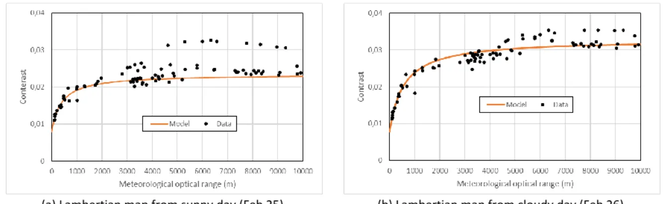
We tried building the Lambertian map with data from before the fog episodes of the Matilda dataset.

We tried with data from February 25, which was a sunny day, and with data from February 26, which

was an overcast day (as observed from the shadows cast by vertical objects in the scene). We can see

in Figure 3 that the Lambertian map built with data from the sunny day fails to improve the tightness

of the data along the response curve, contrary to the weight map from the overcast day. The

estimation errors are presented in Table 3.

(a) Lambertian map from sunny day (Feb 25). (b) Lambertian map from cloudy day (Feb 26).

Figure 3. Influence of the Lambertian map on the response function of the camera-based visibility estimation system. Table 3. 90th _{centile of the relative errors between estimated and reference atmospheric}

visibility, depending on the data which served to build the Lambertian map.

a

b < 400 m

< 1 km

< 2 km

< 5 km < 10 km

Feb 25 (sunny)

0,0156364 385,327

24%

39%

54%

> 100%

> 100%

Feb 26 (overcast)

0,0251376 566,246

32%

46%

62%

76%

79%

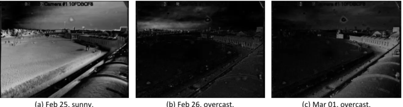
The Lambertian maps are presented in Figure 4. We see that the map from February 25 (sunny) is not

really selective, especially in low contrast areas (the lawn), contrary to the map from February 26

Measurement of Visibility Conditions with Traffic Cameras

(overcast). There are large differences between the map from February 26 and that of March 1,

which is also an overcast day.

(a) Feb 25, sunny. (b) Feb 26, overcast. (c) Mar 01, overcast.

Figure 4. Lambertian maps built with data from days with different sky conditions ((a) sunny and (b) overcast), compared with the original map (c).

Evaluation on different low visibility episodes

Although the Matilda dataset only contains data collected between February 27 and March 1, the

data collection actually started on February 5 and lasted until April 10. There were 7 low visibility

episodes during that period, always around sunrise: February 7, February 21, February 27, February

28, March 5, March 23 and April 4. Having used the data from the episodes of February 27 & 28 to

calibrate the meteorological visibility estimation system, we focused on the last 3 episodes, and then

on the whole period, to evaluate the method. We used the model obtained by fitting low visibility

data without weight (parameters are given in line 3 of Table 1). The data for the last episode and for

the whole period is plotted versus the model in Figure 5.

Table 4. Mean and 90th _{centile of the relative errors between estimated and reference atmospheric visibility,}

for different periods with low visibility episodes (italicized when computed with less than 10 data).

< 400 m

< 1 km

< 2 km

< 5 km

< 10 km

Mar 03-05

11%

29%

11%

25%

15%

33%

16%

33%

53%

94%

Mar 21-23

37%

37%

25%

37%

22%

37%

29%

78%

54%

80%

Apr 01-03

23%

65%

26%

66%

29%

67%

51%

91%

88% > 100%

Mar 02 - Apr 10

16%

33%

17%

33%

20%

55%

42%

86%

74%

91%

Figure 5. Data of April 1-3, computed with the Lambertian map and the model computed from the Matilda dataset.

Discussion

Measurement of Visibility Conditions with Traffic Cameras

to calibrate it. The second limitation is that they applied the Lambertian map backwards in time.

When we apply the calibrated model to estimate visibility from data collected on the same site with

the same camera but at different times (Table 4), or even when we use a Lambertian map computed

from data collected before the data used for the test (Table 3), the results are less accurate, even

when we focus on very low visibility. The shape of the model does however seem to fit the data, only

not as accurately as expected.

We can draw a parallel between the hyperbolic increase of the deviation between estimated and

measured atmospheric visibility and the hyperbolic relation between the distance in the scene and

the line number in the image. With the flat world hypothesis, this relation is:

d = λ / (v – v

)

(7)

where d is the distance from the camera to the ground at line v in the image, and v

is the horizon

line:

v

= v

– tan β

(8)

where v

is the vertical position of the optical center in the image, and β

is the pitch angle of the

camera; λ depends on various characteristics of the camera:

λ = H f / ( µ cos²β

)

(9)

where H is the mounting height, f is the focal length and µ is the pixel size. For the particular camera

installed in Trappes, with H = 8.3 m, β

= 9.8°, f = 4 mm, µ = 9 µm and v

= 240, we have λ = 3799 and

v

= 163. Furthermore, we can estimate the distance δ spanned by one line at distance d:

δ(d) = λ / ( E( v

+ λ / d ) – v

) – λ / ( E( v

+ λ / d ) + 1 – v

)

(10)

where E(x) is the integer part of x. These equations are taken from Hautière et al (2006) and the

parameter values are taken from Hautière et al (2013). We can thus compute the distance beyond

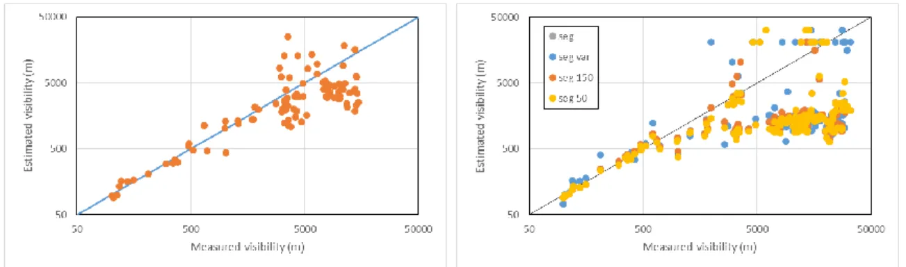
which δ(d) is more than 20% of d, and we find 640 m, which corresponds to the line number 169.

Hypothesizing that it is impossible to get any accuracy from pixels pointing at surfaces beyond that

distance, we tried to compute the unweighted mean of contrast over the lower part of the image,

below line number 169. After calibrating the model proposed by Babari et al (2011) and inversing it

to estimate the visibility from the contrast, we got the results in the graph on the left in Figure 6,

with the 90

_{centile of the relative error at 18% for V < 400 m and 34% for V < 1 km. The parameters}

of the model are a = 0.0225176 and b = 418.636 . We find that the results are similar to what was

obtained on the same dataset (the so-called Matilda dataset) by Caraffa and Tarel (2014) using their

entropy minimization method, as can be seen in the graph on the right in Figure 6.

Figure 6. Visibility estimated from the mean of contrast in the lower part of the image (left), and visibility estimated by entropy minimization as proposed by Caraffa and Tarel (2014) (right), using the Matilda dataset.

Measurement of Visibility Conditions with Traffic Cameras

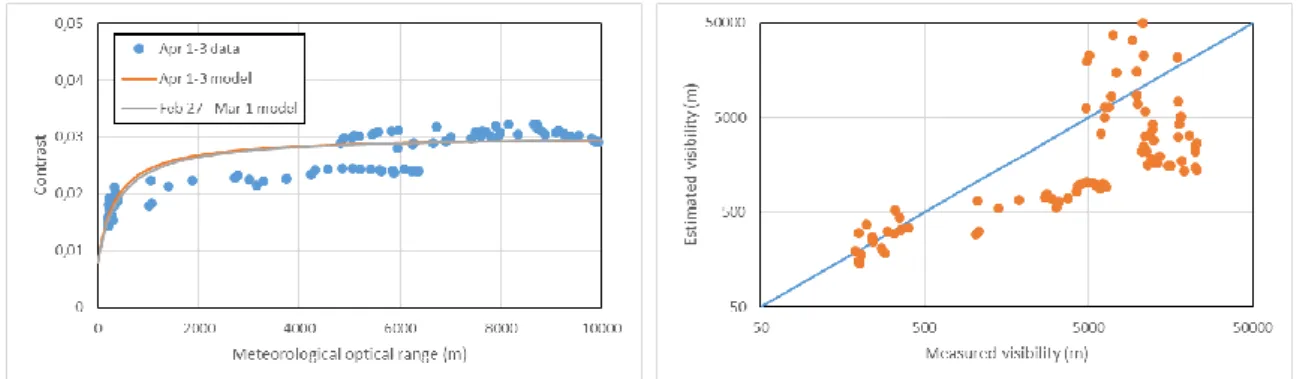
We then tested the model calibrated from the Matilda dataset (i.e. February 27 to March 1st) on

data from the low visibility episode of April 1-3. We found the 90

_{centile of the relative error to be}

higher than 20% even for V < 400 m. We also tried calibrating the model with the data from the April

1-3 episode, but surprisingly, the results were worst (see Figure 7).

Figure 7. Left: average contrast in the lower part of the image as a function of MOR for the April 1-3 episode, with models calibrated from different datasets. Right: visibility estimated with two models versus measured visibility.

The poor quality of the last results led us to question the quality of the reference data. We see in

Figure 8 that the MOR, as measured with a scatter meter, varies literally by the minute, although the

measurements are actually averaged over 6 minutes to smooth out non-significant instantaneous

variations. The visibility estimated with the camera, on the other hand, is an instantaneous value.

Therefore, we should also test averaging the results extracted from several images. Unfortunately,

only 1 image every 10 minutes were collected in Trappes, so we need new data to pursue this line of

investigation.

Figure 8. Variations of MOR between 08:00 and 10:00 in the morning of 3 low visibility episodes (the dots correspond to the values that are associated with images).

Meanwhile, we tried using the median value of the MOR over 10-minute periods around the time

each image was captured. The results were noticeably improved, as can be seen in Figure 9, although

the 90

_{centile of the relative error is still 58% for V < 400 m and 65% for V < 2 km (there is no data}

for V between 400 m and 1 km). The parameters of the model are a = 0.0223199 and b = 357.314 ,

which is quite close to the model obtained earlier with the data from the Matilda dataset using the

contrast in the lower part of the image. This raises our hopes that the model calibrated using a low

visibility episode might remain valid for later episodes.

Measurement of Visibility Conditions with Traffic Cameras

Figure 9. Left: data and model for the April 1-3 episode using the median value of the MOR over 10’ periods, along with the model from the Matilda dataset. Right: visibility estimated by inversing the model, versus measured visibility.

Conclusions and future work

We have implemented the physically based method proposed by Babari et al (2011) to estimate

atmospheric visibility from the weighted mean of contrast in the image of a scene captured by a

CCTV camera. We found that the so-called Lambertian weight map does not successfully suppress

the influence of illumination in the scene outside the time frame originally tested by the authors.

Simply using the mean of contrast below a certain line in the image seems to provide results with

similar accuracy. We also found that calibrating the model outside the timeframe originally tested by

the authors does not always produce an acceptable model (one that can be inversed to estimate

visibility from contrast with reasonable accuracy). However, it does not necessarily follow that the

method is invalid: imprecision in the results may come from the instantaneous nature of the

computed contrast, compared to the reference data where visibility is averaged over a period of

several minutes. The same remark holds for the more recent method proposed by Caraffa and Tarel

(2014). Whatever the method, it seems impossible to obtain reasonably accurate results beyond a

certain visibility value which depends on the intrinsic and extrinsic characteristics of the camera

(basically its resolution, mounting height and pitch angle).

We have started collecting data from other sites to complete the evaluation of the camera based

visibility estimation method(s). When possible, we will collect sequences of images (e.g. 10 images at

1 Hz) instead of single frames every 10 minutes, in order to smooth out non-significant variations.

We will also need to estimate the depth map of the scene when possible (e.g. using a stereo vision

system), in order to explore the possibility of building the model relating contrast and visibility

without need for the reference visibility data required for calibration as proposed in Babari’s PhD

thesis (2012).

There are several things that we want to investigate in future work. First, we want to look into the

definition of the local contrast that we extract in the images. Up to this point, we have implemented

a contrast which is actually a gradient (as can be seen in Equation 5). Other possibilities are listed in

Hautiere’s early work (2005) which might be more relevant for computing contrast maps. We will

also consider visibility level as an alternative to contrast (Tarel et al, 2015). Secondly, we want to look

into the two-steps calibration method of calibrating the response curve of the camera proposed in

Babari’s PhD thesis (2012): 1. implement a calibration-free meteorological visibility estimation

method which gives reasonably accurate results for very low visibility conditions, such as the

inflection point method (Hautiere, 2005) or the entropy minimization method (Caraffa and Tarel,

2014), to learn the slope of the lower part of the response curve, i.e. a/b from Equation (6); 2. Use

images acquired in the best visibility conditions to learn the asymptotic value of the response curve,

i.e. a+c from Equation (6).

Measurement of Visibility Conditions with Traffic Cameras

Acknowledgements

This project was initiated by Ifsttar in 2008 with Raouf Babari’s PhD, co-funded by Meteo-France and

co-supervised by IGN. A grant from Institut Carnot VITRES made it possible in 2013 to recruit

Abderraouf Zermane to program the visibility estimation method in C language. The work has been

pursued in the framework of Ifsttar’s COMET research project.

References

Raouf Babari, Nicolas Hautière, Eric Dumont, Roland Brémond, Nicolas Paparoditis. A model-driven

approach to estimate atmospheric visibility with ordinary cameras. Atmospheric Environment,

Elsevier, 2011, 45(30), pp. 5316-5324. <10.1016/i.atmosenv.2011.06.053>.

Laurent Caraffa and Jean Philippe Tarel. Daytime Fog Detection and Density Estimation with Entropy

Minimisation. ISPRS Annals of Photogrammetry, Remote Sensing and Spatial Information Sciences,

2014, II(3), pp. 25-31. < 10.5194/isprsannals-II-3-25-2014>

Nicolas Hautière, Jean-Philippe Tarel, Jean Lavenant and Didier Aubert. Automatic fog detection and

estimation of visibility distance through use of an onboard camera. Machine Vision and Applications,

2006, 17(1), pp. 8-20. <10.1007/s00138-005-0011-1>

Nicolas Hautière, Raouf Babari, Eric Dumont, Jacques Parent Du Chatelet and Nicolas Paparoditis.

Measurements and Observations of Meteorological Visibility at ITS Stations. In Yuanzhi Zhang &

Pallav Ray (ed.), InTech (pub.): Climate Change and Regional/Local Responses, 2013, pp. 89-108.

<10.5772/55697>.

John R. Taylor and Jamie C. Moogan. Determination of visual range during fog and mist using digital

camera images. IOP Conference Series: Earth and Environmental Science, 2010, 11(1).

<10.1088/1755-1315/11/1/012012>.

Joachim Wuttke: lmfit – a C library for Levenberg-Marquardt least-squares minimization and curve

fitting. Version 6.1, retrieved on December 15, 2016, from

http://apps.jcns.fz-juelich.de/lmfit

.

Ling Xie, Alex Chiu and Shawn Newsam. Estimating Atmospheric Visibility Using General-Purpose

Cameras. In G. Bebis et al (ed.): International Symposium on Visual Computing, 2008, Part II, pp.

356-367. < 10.1007/978-3-540-89646-3_35>.

Raouf Babari. Estimation des conditions de visibilité météorologique par caméras routières. Mémoire

de thèse de doctorat, Université Paris Est (ED MSTIC), 2012.

Nicolas Hautiere. Détection des conditions de visibilité et estimation de la distance de visibilité par

vision embarquée. Mémoire de thèse de doctorat, Université Jean Monnet de Saint-Etienne, 2005.

Jean Philippe Tarel, Roland Bremond, Eric Dumont and Karine Joulan. Comparison between optical

and computer vision estimates of visibility in daytime fog. In Proceedings of the 28th Session of the

CIE (CIE 216:2015), 2015, pp. 610-617.

Appendix 1: program codes

Object: selects images acquired in a given period (based on their timestamp) in given weather conditions (based on weather data, specially visibility and luminance).

Syntax: .\dosel sel_in.txt > sel_out.txt

Input: arguments are provided by means of an ASCII file (sel_in.txt); the parameters are documented in the comments of that file.

Output: the matching images are listed with the weather data in an ASCII file (sel_out.txt) which can then serve to compute the Lambertian surface map, to calibrate the camera-based visibility meter or to test the results.

domap.c (page 9)

Object: computes the time correlation between pixel intensity and a given weather parameter (normally luminance, or sun elevation) as an indicator of the Lambertian character of surfaces, from data selected using DOSEL.

Syntax: .\domap map_in.txt

Input: arguments are provided by means of an ASCII file (map_in.txt). The parameters are documented in the comments of that file.

Output: the map of Lambertian surfaces is stored into a PFM file, the name of which is specified in the input file.

docal.c (page 14)

Object: computes the parameters of the response function of the camera-based visibility meter, from data selected using DOSEL.

Syntax: .\docal cal_in.txt > cal_out.txt

Input: arguments are provided by means of an ASCII file (cal_in.txt). The parameters are documented in the comments of that file.

Output: the weighted mean of gradient in each image is given (to plot the response) are stored into an ASCII file, at the end of which and the values of the model parameters are given.

dotst.c (page 20)

Object: computes the error between estimated and reference visibility with data selected using DOSEL.

Syntax: .\dotst tst_in.txt > tst_out.txt

Input: arguments are provided by means of an ASCII file (tst_in.txt). The parameters are documented in the comments of that file.

Output: the mean and the 90th-centile of the relative error are tabulated for several classes of visibility.

/*

CAM2 toolbox: DOSEL ===================

Object: selects images acquired in a given period (based on their timestamp) in given weather conditions (based on weather data, specially visibility and luminance).

Syntax: .\dosel sel_in.txt > sel_out.txt

Input: arguments are provided by means of an ASCII file (sel_in.txt); the parameters are documented in the comments of that file.

Output: the matching images are listed with the weather data in an ASCII file (sel_out.txt) which can then serve to compute the Lambertian surface map, to calibrate the camera-based visibility meter or to test the results.

*/ #include <stdio.h> #include <string.h> #include <time.h> #include <sys/stat.h> #include <math.h> #define BUFSIZE 1024 #define PI 3.14159265358979323846 #define RAD (PI/180)

#define TWOPI (2*PI)

#define EMR 6371.01 // earth mean radius in km #define AU 149597890 // astronomical unit in km typedef struct struct_data

{

int valid; // 1 for valid data, 0 for invalid data int hour; int min; int sec; float vi; float bl; } type_data;

#define sizeof_data sizeof(type_data) typedef unsigned char uchar;

const char * codestr[] = { "Date\0", "Time\0", "VI\0", "BL\0" }; typedef enum { codeDate = 0, codeTime = 1, codeVI = 2, codeBL = 3 } type_code;

#define Oops(m) {fprintf(stderr, "\n\nOops! %s\n\n", m); exit(-1);} #define Warn(m) {fprintf(stderr, "\n\nHum... %s\n\n", m);}

// from http://www.psa.es/sdg/sunpos.htm float SunPos(float longitude, float latitude,

int year, int mon, int mday, int hour, int min, int sec) { // Main variables double dElapsedJulianDays; double dDecimalHours; double dEclipticLongitude; double dEclipticObliquity; double dRightAscension; double dDeclination; double dZenithAngle; double dAzimuth; // Auxiliary variables double dY; double dX;

// Calculate difference in days between the current Julian Day // and JD 2451545.0, which is noon 1 January 2000 Universal Time {

double dJulianDate; long int liAux1; long int liAux2;

// Calculate time of the day in UT decimal hours dDecimalHours = hour + (min + sec / 60.0 ) / 60.0; // Calculate current Julian Day

liAux1 = (mon-14)/12;

liAux2 = (1461*(year + 4800 + liAux1))/4 + (367*(mon-2-12*liAux1))/12 - (3*((year + 4900 + liAux1)/100))/4 + mday-32075;

// Calculate ecliptic coordinates (ecliptic longitude and obliquity of the // ecliptic in radians but without limiting the angle to be less than 2*Pi // (i.e., the result may be greater than 2*Pi)

{

double dMeanLongitude; double dMeanAnomaly; double dOmega;

dOmega = 2.1429-0.0010394594*dElapsedJulianDays;

dMeanLongitude = 4.8950630+ 0.017202791698*dElapsedJulianDays; // Radians dMeanAnomaly = 6.2400600+ 0.0172019699*dElapsedJulianDays;

dEclipticLongitude = dMeanLongitude + 0.03341607*sin( dMeanAnomaly ) + 0.00034894*sin( 2*dMeanAnomaly )-0.0001134

-0.0000203*sin(dOmega);

dEclipticObliquity = 0.4090928 - 6.2140e-9*dElapsedJulianDays +0.0000396*cos(dOmega);

}

// Calculate celestial coordinates ( right ascension and declination ) in radians // but without limiting the angle to be less than 2*Pi (i.e., the result may be // greater than 2*Pi)

{

double dSin_EclipticLongitude;

dSin_EclipticLongitude = sin( dEclipticLongitude ); dY = cos( dEclipticObliquity ) * dSin_EclipticLongitude; dX = cos( dEclipticLongitude );

dRightAscension = atan2( dY,dX );

if( dRightAscension < 0.0 ) dRightAscension = dRightAscension + TWOPI; dDeclination = asin( sin( dEclipticObliquity )*dSin_EclipticLongitude ); }

// Calculate local coordinates ( azimuth and zenith angle ) in degrees { double dGreenwichMeanSiderealTime; double dLocalMeanSiderealTime; double dLatitudeInRadians; double dHourAngle; double dCos_Latitude; double dSin_Latitude; double dCos_HourAngle; double dParallax; dGreenwichMeanSiderealTime = 6.6974243242 + 0.0657098283*dElapsedJulianDays + dDecimalHours;

dLocalMeanSiderealTime = (dGreenwichMeanSiderealTime*15 + longitude)*RAD; dHourAngle = dLocalMeanSiderealTime - dRightAscension;

dLatitudeInRadians = latitude*RAD;

dCos_Latitude = cos( dLatitudeInRadians ); dSin_Latitude = sin( dLatitudeInRadians ); dCos_HourAngle= cos( dHourAngle );

dZenithAngle = (acos( dCos_Latitude*dCos_HourAngle

*cos(dDeclination) + sin( dDeclination )*dSin_Latitude)); dY = -sin( dHourAngle );

dX = tan( dDeclination )*dCos_Latitude - dSin_Latitude*dCos_HourAngle; dAzimuth = atan2( dY, dX );

if ( dAzimuth < 0.0 )

dAzimuth = dAzimuth + TWOPI; dAzimuth = dAzimuth/RAD;

// Parallax Correction

dParallax = (EMR/AU) * sin(dZenithAngle); dZenithAngle = (dZenithAngle + dParallax)/RAD; }

return 90.0-dZenithAngle; // solar elevation }

time_t settime(int year, int month, int day, int hour, int minute, int second) { /*================*/ struct tm *timeinfo; time_t rawtime; int week; char buf[4]; /*================*/ time ( &rawtime );

timeinfo = gmtime ( &rawtime );

timeinfo->tm_year = year-1900; // year since 1900 timeinfo->tm_mon = month-01; // month since January timeinfo->tm_mday = day;

timeinfo->tm_hour = hour; timeinfo->tm_min = minute; timeinfo->tm_sec = second;

rawtime = mkgmtime(timeinfo); // make sure all fields of the tm struct are ok

return rawtime; }

int getWeek(int year, int month, int day) { /*================*/ struct tm *timeinfo; time_t rawtime; int week; char buf[4]; /*================*/ time ( &rawtime );

timeinfo = gmtime ( &rawtime );

timeinfo->tm_year = year-1900; // year since 1900 timeinfo->tm_mon = month-01; // month since January timeinfo->tm_mday = day;

rawtime = mkgmtime(timeinfo); // make sure all fields of the tm struct are ok timeinfo = gmtime ( &rawtime );

strftime(buf, 4, "%W", timeinfo); sscanf(buf, "%d", &week);

//printf("\n%s => week nb %d", asctime(timeinfo), week+1); return week+1;

}

int readWeatherData(char *filename, type_data *data, int *indexVI, int *indexBL) {

/*================*/ FILE *f;

char buf[BUFSIZE]; char *ptr, str[5];

int nbparam, p, nbdata, i; type_code *codeparam; float value;

int year, mon, mday, hour, min, sec, t; /*================*/

// open file

f = fopen(filename, "rt");

if (!f) return 0; // no (*data) file by that name

// read the head line

if (!fgets(buf, BUFSIZE, f)) {

fclose(f);

return 0; // empty (*data) file }

// count parameters in the head line // knowing they are seperated by tabs // (Date and Time are the first 2) nbparam = 1; ptr = strchr(buf, '\t'); while (ptr) { nbparam++; ptr = strchr(ptr+1, '\t'); }

// printf("\n %s contains %d parameters.", strrchr(filename, '\\')+1, nbparam-2); codeparam = (type_code*)malloc(nbparam*sizeof(int));

if (!codeparam) Oops("Not enough memory.");

// identify the parameters from their code *indexVI = *indexBL = -1; ptr = buf; for (p=0; p<nbparam; p++) { sscanf(ptr, "%s", str); if (!strcmp(str, "Date")) codeparam[p] = codeDate; else if (!strcmp(str, "Time")) codeparam[p] = codeTime; else if (!strcmp(str, "VI")) { codeparam[p] = codeVI; *indexVI = p; } else if (!strcmp(str, "BL")) { codeparam[p] = codeBL; *indexBL = p; } else Oops("Unknown paramater.");

// if ((*indexBL)>0) printf(" BL@%d", *indexBL); if (((*indexVI)<0) || ((*indexBL)<0))

{

fclose(f); free(codeparam);

Warn("No visibility (VI) or luminance (BL) in (*data) file."); return 0; // neither visibility nor luminance

}

// count the lines, i.e. (*data) points // to allocate memory

nbdata = 0;

while (fgets(buf, BUFSIZE, f)) nbdata++;

if (nbdata<1) return 0; // No (*data) // printf("\n There are %d items.", nbdata);

// initialize data array for (hour=0; hour<24; hour++) for (min=0; min<60; min++) data[hour*60+min].valid = 0;

// rewind, and read the (*data) rewind(f);

fgets(buf, BUFSIZE, f); // skip head line for (i=0; i<nbdata; i++)

{

if (fscanf(f, "%d/%d/%d %d:%d:%d",

&year, &mon, &mday, &hour, &min, &sec)<6)

Oops("Data format error (yyyy/mm/dd hh:mm:ss)."); t = hour*60+min; data[t].hour = hour; data[t].min = min; data[t].sec = sec; for (p=2; p<nbparam; p++) { if (fscanf(f, "%f", &value)<1)

Oops("Data format error (numerical values)."); if (p==(*indexVI)) data[t].vi = value;

else if (p==(*indexBL)) data[t].bl = value; } data[t].valid = 1; } fclose(f); // clean memory free(codeparam); return nbdata; }

int searchWeatherData(type_data *data, int i_hour, int i_min, int i_sec, int *w_timer) { /*================*/ int dt1, dt2; int t, t1, t2; /*================*/ // image timer t = *w_timer = i_hour*60+i_min;

// check for exact match if (data[t].valid) return 1;

// go back 6 mins dt1 = 1;

while ((dt1<6) && (t1-dt1>=0) && (!(data[t-dt1].valid))) dt1++;

// go forth 6 mins dt2 = 1;

while ((dt2<6) && (t+dt2<1440) && (!(data[t+dt2].valid))) dt2++;

// choose the closest in time if (dt1<dt2)

*w_timer = t-dt1; else if (dt2<dt1) *w_timer = t+dt2;

else return 0; // no matching timestamp with 12 min return 1;

}

float getVisibilityIndicator(char *filename, int wmin, int hmin, int wmax, int hmax) {

/*================*/ FILE *f;

int width, height; int w, h, x, y; uchar **image, imax; float dLx, dLy, g, m;

// use Sobel operator to approximate first derivative

float Kx[3][3] = {{+0.25, 0.0, -0.25}, {+0.5, 0.0, -0.5}, {+0.25, 0.0, -0.25}}; float Ky[3][3] = {{+0.25, +0.5, +0.25}, { 0.0, 0.0, 0.0}, {-0.25, -0.5, -0.25}}; /*================*/

// check window

if ((wmin<=0) || (wmax>=width) || (hmin<=0) || (hmax>=height)) // convert image to pgm file format

if (!system(NULL)) Oops("Cannot execute command.");

sprintf(buf, "C:\\prgm\\ImageMagick-6.8.8-7\\convert.exe %s tmp.pgm", filename); system(buf);

// read image

f = fopen("tmp.pgm", "rb");

if (!f) Oops("Image conversion failed.");

if (!fgets(buf, BUFSIZE, f)) Oops("Empty PGM file.");

if (strncmp(buf, "P5", 2)) Oops("Not a binary PGM file (P5)."); if (!fgets(buf, BUFSIZE, f)) Oops("Unexpected end of PGM file.");

if (sscanf(buf, "%d %d", &width, &height)<2) Oops("PGM header error (size)."); if (!fgets(buf, BUFSIZE, f)) Oops("Unexpected end of PGM file.");

if (sscanf(buf, "%u", &imax)<1) Oops("PGM header error (max value)."); image = (uchar**)malloc(height*sizeof(uchar*));

if (!image) Oops("Not enough memory for image."); for (h=0; h<height; h++)

{

image[h] = (uchar*)malloc(width*sizeof(uchar));

if (!(image[h])) Oops("Not enough memory for image line."); if (fread(image[h], width*sizeof(uchar), 1, f)<1)

Oops("Failed to read image from file."); }

fclose(f);

// compute mean gradient module m = 0.0;

for (h=hmin; h<=hmax; h++) for (w=wmin; w<=wmax; w++) {

dLx = 0; dLy = 0;

for (y=-1; y<=1; y++) for (x=-1; x<=1; x++) {

dLx += Kx[1+y][1+x] * (float)image[h+y][w+x]; dLy += Ky[1+y][1+x] * (float)image[h+y][w+x]; } m += sqrt(dLx*dLx+dLy*dLy); } // clean memory for (h=0; h<height; h++) free(image[h]); free(image); return m/(float)(wmax-wmin+1)/(float)(hmax-hmin+1)/(float)imax; }

int main(int argc, char **argv) {

/*================*/ FILE *f;

struct stat fileinfo;

char buf[BUFSIZE], path[BUFSIZE], ifile[BUFSIZE], dfile[BUFSIZE]; int nbDays;

type_code *codeparam;

type_data wdata[1440]; // allocate for 1day=24h*60min max of measurements int nbdata, indexVI, indexBL;

float longitude, latitude;

float S; // sun position (sun elevation) float L, Lmin=-1, Lmax = -1; // luminance float V, Vmin=-1, Vmax = -1; // visibility

int yy, mm, ww, dd, yy1, mm1, ww1, dd1=-1, yy2, mm2, ww2, dd2=-1; int d, h, h1, h2, m, m1, m2, s, i, t;

int wh, wm;

int set_Date, set_Time, set_VI, set_BL, set_Path, set_Pos; time_t tt, tt1, tt2;

struct tm *ti; /*================*/

*/

f = fopen(argv[1], "rt");

if (!f) Oops("Input file not found.");

set_Date = set_Time = set_VI = set_BL = set_Path = 0; path[0] = '\0';

while (fgets(buf, BUFSIZE, f)) {

if (buf[0] != '#') {

if (strstr(buf, "Date")) {

if (sscanf(buf, "Date from %4d/%2d/%2d to %4d/%2d/%2d", &yy1, &mm1, &dd1, &yy2, &mm2, &dd2)<6)

Oops("Error at date."); set_Date = 1;

// printf("\n d1 = %4d/%02d/%02d", yy1, mm1, dd1); // printf("\n d2 = %4d/%02d/%02d", yy2, mm2, dd2); }

else if (strstr(buf, "Time")) {

if (sscanf(buf, "Time between %2d:%2d and %2d:%2d", &h1, &m1, &h2, &m2)<4)

Oops("Error at time (wrong format)."); if ( (h1<0)||(h2<0)||(h1>23)||(h2>23) ||(m1<0)||(m2<0)||(m1>59)||(m2>59)) Oops("Error at time (out of range)."); set_Time = 1;

// printf("\n t1 = %02d:%02d", h1, m1); // printf("\n t2 = %02d:%02d", h2, m2); }

else if (strstr(buf, "Luminance")) {

if (sscanf(buf, "Luminance from %f to %f", &Lmin, &Lmax)<2) Oops("Error at Lmin.");

set_BL = 1;

// printf("\n %g <= L < %g", Lmin, Lmax); }

else if (strstr(buf, "Visibility")) {

if (sscanf(buf, "Visibility from %f to %f", &Vmin, &Vmax)<2) Oops("Error at Vmin.");

set_VI = 1;

// printf("\n %g <= V < %g", Vmin, Vmax); }

else if (strstr(buf, "Path")) {

strcpy(path, strchr(buf, ' ')+1);

if ((strlen(path)<2) || (strlen(path)>BUFSIZE-2)) Oops("Error at path.");

path[strlen(path)-1] = '\0';

// printf("\n path = %s !", path);

if (stat(path, &fileinfo)<0) Oops("Invalid path."); set_Path = 1;

}

else Oops("Unknown parameter in input file."); }

} fclose(f);

if ((!set_Date) || (!set_Time) || (!set_BL) || (!set_VI) || (!set_Path)) Oops("Missing parameter(s).");

/*

// find weather station description in path/ */

sprintf(buf, "%s\\%s.txt", path, strrchr(path, '\\')+1); f = fopen(buf, "rt");

if (!f) Oops("Description of weather station not found."); while (fgets(buf, BUFSIZE, f))

{

if (buf[0] != '#') {

if (strstr(buf, "Position")) {

if (sscanf(buf, "Position %f %f", &latitude, &longitude)<2) Oops("Error at position in station description file."); set_Pos = 1;

// printf("\n position = %g, %g", latitude, longitude); } } } fclose(f); if ((!set_Pos)) Oops("Missing parameter(s)."); // output header

printf("# Selection parameters:\n"); printf("# Path = %s \n", path);

printf("# Location: %c %f , %c %f \n", (latitude<0)?'S':'N', latitude, (longitude<0)?'W':'E', longitude);

printf("# Time period: %4d/%02d/%02d (%02d)", yy1, mm1, dd1, ww1 = getWeek(yy1, mm1, dd1));

printf(" to %4d/%02d/%02d (%02d) \n", yy2, mm2, dd2, ww2 = getWeek(yy2, mm2, dd2)); printf("# %02d:%02d <= T <= %02d:%02d \n", h1, m1, h2, m2);

printf("# %g <= L (cd/m2) < %g \n", Lmin, Lmax); printf("# %g <= V (m) < %g \n", Vmin, Vmax); printf("Image\tDate\tTime\tSE\tBL\tVI\n");

/*

// find image and (*data) files in path/yyyy/ww/ */

tt1 = settime(yy1, mm1, dd1, 0, 0, 0); tt2 = settime(yy2, mm2, dd2, 23, 59, 59); nbDays = ((int)difftime(tt2, tt1)+1)/(24*60*60); // printf("\n %d => %d (%d days)", tt1, tt2, nbDays); tt = tt1; nbdata = 0; for (d=0; d<nbDays; d++) { ti = gmtime(&tt); // printf(" %d ", tt); yy = ti->tm_year+1900; mm = ti->tm_mon+1; dd = ti->tm_mday;

ww = getWeek(yy, mm, dd); // warning: getWeek resets ti (!?) sprintf(dfile, "%s\\%4d\\%02d\\%4d%02d%02d.txt",

path, yy, ww, yy, mm, dd);

// if (*data) file exists and actually contains (*data), then look for images if (readWeatherData(dfile, wdata, &indexVI, &indexBL))

{

for (h=0; h<24; h++) for (m=0; m<60; m++) for (s=0; s<60; s++) if ((h*60+m>=h1*60+m1)&&(h*60+m<=h2*60+m2)) { sprintf(ifile, "%s\\%4d\\%02d\\%4d%02d%02d%02d%02d%02d.jpg", path, yy, ww, yy, mm, dd, h, m, s);

// if (f=fopen(ifile, "r")) { fclose(f); printf("\n %s", ifile);} if (!stat(ifile, &fileinfo)) // image file found

{

// printf("\n %s => %s", strrchr(dfile, '\\')+1, strrchr(ifile, '\\')+1); // look for data with similar timestamp

if ((searchWeatherData(wdata, h, m, s, &t))) {

L = wdata[t].bl; V = wdata[t].vi;

S = SunPos(longitude, latitude, yy, mm, dd, h, m, s);

// fprintf(stderr, "%s\t%g\t%g\n", strrchr(ifile, '\\')+1, V, L); if ( (V >= Vmin) && (V < Vmax)

&& (L >= Lmin) && (L < Lmax)) { printf("%s\t%4d/%02d/%02d\t%02d:%02d:%02d\t%g\t%g\t%g\n", ifile, yy, mm, dd, h, m, s, S, L, V); // getVisibilityIndicator(ifile, 16, 32, 616, 472); nbdata++; } }

// else printf(" => no data within 12 min"); } } } // go to next day tt += 24*60*60; }

if (nbdata) fprintf(stderr, "\n %d matching data found.", nbdata); else fprintf(stderr, "\n No match.");

fprintf(stderr, "\n\n No problemo. \n\n"); return 0;

/*

CAM2 toolbox: DOMAP ===================

Object: computes the time correlation between pixel intensity and a given weather parameter (normally luminance, or sun elevation) as an indicator of the Lambertian character of surfaces, from data selected using DOSEL.

Syntax: .\domap map_in.txt

Input: arguments are provided by means of an ASCII file (map_in.txt). The parameters are documented in the comments of that file.

Output: the map of Lambertian surfaces is stored into a PGM file, the name of which is specified in the input file.

*/ #include <stdio.h> #include <string.h> #include <time.h> #include <sys/stat.h> #include <math.h> #define BUFSIZE 2048 typedef unsigned char uchar; typedef enum IndEnum

{

NONE=0, // weight = 1

CORR=1, // weight = squared correlation with luminance (or other parameter) PCOR=2, // weight = squared positive correlation

NCOR=3, // weight = squared negative correlation ASDV=4, // weight = std-deviation of contrast

RSDV=5 // weight = relative std-deviation of contrast } indType;

#define Oops(m) {fprintf(stderr, "\n\nOops! %s\n\n", m); exit(-1);} #define Warn(m) {fprintf(stderr, "\n\nHum... %s\n\n", m);}

void readPGM(char *name, uchar ***data, int *width, int *height) { /*---*/ FILE *f; int h, w; char buf[256]; /*---*/ f = fopen(name, "rb");

if (!f) Oops("File not found."); fgets(buf, 256, f);

if (!strstr(buf, "P5")) Oops("Not a PGM file."); while ((fgets(buf, 256, f))&&(buf[0]=='#')); sscanf(buf, "%d %d", width, height);

fgets(buf, 256, f);

(*data) = (uchar**)malloc((*height)*sizeof(uchar*)); if (!(*data)) Oops("Not enough memory.");

for (h=0; h<*height; h++) {

(*data)[h] = (uchar*)malloc((*width)*sizeof(uchar)); if (!((*data)[h])) Oops("Not enough memory.");

if (fread((*data)[h], (*width)*sizeof(uchar), 1, f)<1) Oops("Read error.");

} fclose(f); }

void writePFM(char *pfm, float **data, int width, int height, char *str, float total) { /*---*/ FILE *f; int h, w; int doflip = 0; float s; /*---*/ f = fopen(pfm, "wb");

fprintf(f, "Pf\n# Created using dolamb\n"); fprintf(f, "# Indicator: %s\n", str); if (total<0) { s = 0.0; for (h=0; h<height; h++) for (w=0; w<width; w++) s += data[h][w]; } else s = total; fprintf(f, "# Total: %g\n", s);

fprintf(f, "%d %d\n-1\n", width, height); if (doflip)

else

for (h=0; h<height; h++) fwrite(data[h], width*sizeof(float), 1, f); fclose(f);

}

int main(int argc, char **argv) {

/*================*/

char * parcodestr[] = { "Image\0", "Date\0", "Time\0", "SE\0", "BL\0", "VI\0" }; char * indcodestr[] = { "none\0", "corr\0", "pcor\0", "ncor\0", "asdv\0", "rsdv\0" }; FILE *f;

fpos_t marker;

char buf[BUFSIZE], filename[BUFSIZE], infile[BUFSIZE], outfile[BUFSIZE], cmdstr[BUFSIZE]; int set_In=0, set_Win=0, set_Par=0, set_Out=0, set_Cmd=0;

indType set_Ind=0;

char *ptr, date[11], time[9]; int nbIma, n, p;

int w, width, h, height;

int wmin=16, hmin=32, wmax=616, hmax=472; // values for the Trappes database uchar ***ima;

float **map; float *lum;

float ml, sll, x, totalWeight; float **mi, **sii, **sil; /*================*/

if (argc<2) Oops("Syntax: .\\domap.exe domap.txt");

/*

// read input parameters from file (argv[1]) */

f = fopen(argv[1], "rt");

if (!f) Oops("Input file not found."); set_In = set_Win = set_Par = set_Out = 0; set_Ind = NONE;

while (fgets(buf, BUFSIZE, f)) { if (buf[0] != '#') { if (strstr(buf, "Selection")) { strcpy(infile, strrchr(buf, ' ')+1); if ((strlen(infile)<2) || (strlen(infile)>BUFSIZE-2)) Oops("Error at selection filename.");

infile[strlen(infile)-1] = '\0'; printf("\n list = %s", infile); set_In = 1;

}

else if (strstr(buf, "Window")) {

if (sscanf(buf, "Window: %d %d %d %d", &wmin, &wmax, &hmin, &hmax)<4) Oops("Error at window coordinates.");

set_Win = 1;

printf("\n window = (%d,%d)->(%d,%d)", wmin, hmin, wmax, hmax); }

else if (strstr(buf, "Indicator")) {

if (strstr(buf, "none")) set_Ind = NONE;

else if (strstr(buf, "correlation")) set_Ind = CORR; else if (strstr(buf, "positive")) set_Ind = PCOR; else if (strstr(buf, "negative")) set_Ind = NCOR; else if (strstr(buf, "absolute")) set_Ind = ASDV; else if (strstr(buf, "relative")) set_Ind = RSDV; else Oops("Unknown Lambertian indicator.");

printf("\n indicator = %s", indcodestr[set_Ind]); }

else if (strstr(buf, "Parameter")) {

if (sscanf(buf, "Parameter index: %d", &set_Par)<1) Oops("Error at parameter index.");

set_Par -= 1;

printf("\n parameter = %s", parcodestr[set_Par]); }

else if (strstr(buf, "Save map")) {

strcpy(outfile, strrchr(buf, ' ')+1);

if ((strlen(outfile)<2) || (strlen(outfile)>BUFSIZE-2)) Oops("Error at output filename.");

outfile[strlen(outfile)-1] = '\0'; printf("\n output = %s", outfile); set_Out = 1;

}

cmdstr[strlen(cmdstr)-1] = '\0'; printf("\n cmd = %s", cmdstr); set_Cmd = 1;

}

else Oops("Unknown parameter in input file."); }

} fclose(f);

if ((!set_In) || (!set_Win) || ((set_Ind==CORR) && (!set_Par)) || (!set_Out) || (!set_Cmd))

Oops("Missing parameter(s).");

if (set_Ind>NCOR) Oops("The contrast-based indicators are not implemented.");

/*

// look at selected images and associated data to build weight map */

// read selection

f = fopen(infile, "rt");

if (!f) Oops("List file not found."); // skip header

buf[0] = '#'; while (buf[0]=='#')

if (!fgets(buf, BUFSIZE, f)) Oops("Unexpected end of file."); // TODO: check presence of parameter

// count items

fgetpos(f, &marker); // set marker nbIma = 0;

while (fgets(buf, BUFSIZE, f)) nbIma++; if (!nbIma) Oops("Empty list.");

fsetpos(f, &marker); // rewind to marker // printf("\n %d items\n", nbIma); // read images

ima = (uchar***)malloc(nbIma*sizeof(uchar**)); if (!ima) Oops("Not enough memory for images."); lum = (float*)malloc(nbIma*sizeof(float));

if (!lum) Oops("Not enough memory for lum data."); for (n=0; n<nbIma; n++)

{

if (!fgets(buf, BUFSIZE, f)) Oops("Unexpected end of file."); // read filename (1st column) and parameter to correlate strcpy(filename, buf); *(strchr(filename, '\t')) = '\0'; // printf("\n %s", strrchr(filename, '\\')+1); ptr = strchr(buf, '\t'); for (p=1; p<set_Par; p++) ptr = strchr(ptr+1, '\t'); // printf(" %d", p); if ((!ptr) || (sscanf(ptr, "%f\t", &(lum[n]))<1)) Oops("Could not find parameter.");

// printf(" %g", lum[n]);

// convert image to pgm file format

if (!system(NULL)) Oops("Cannot execute command."); sprintf(buf, "%s %s tmp.pgm", cmdstr, filename); system(buf);

// read image

readPGM("tmp.pgm", &(ima[n]), &w, &h); if (n==0)

{

width = w; height = h; /*

// "Empty" map => weight=1 inside the processed window, 0 elsewhere */

if (!set_Ind) {

map = (float**)malloc(height*sizeof(float*));

if (!map) Oops("Not enough memory for lamb map based on luminance."); for (h=0; h<height; h++)

{

map[h] = (float*)malloc(width*sizeof(float));

if (!(map[h])) Oops("Not enough memory for lamb map."); for (w=0; w<width; w++) { if ((w>=wmin)&&(w<=wmax)&&(h>=hmin)&&(h<=hmax)) map[h][w] = 1.0; else map[h][w] = 0.0; } }

writePFM(outfile, map, width, height, indcodestr[set_Ind], (wmax-wmin+1)*(hmax-hmin+1));

for (h=0; h<height; h++) free(map[h]); free(map); free(ima); free(lum); fclose(f); fprintf(stderr, "\n\n No problemo. \n\n"); return 0; // Bye bye } }

else if ((w!=width) || (h!=height)) Oops("Images with different sizes."); }

fclose(f);

// compute means of intensity, gradient and luminance mi = (float**)malloc(height*sizeof(float*));

if (!mi) Oops("Not enough memory for pixel mean."); for (h=0; h<height; h++)

{

mi[h] = (float*)malloc(width*sizeof(float));

if (!(mi[h])) Oops("Not enough memory for pixel mean."); }

for (h=hmin; h<=hmax; h++) for (w=wmin; w<=wmax; w++) { mi[h][w] = 0.0; for (n=0; n<nbIma; n++) mi[h][w] += (float)(ima[n][h][w]); mi[h][w] /= (float)nbIma; } ml = 0.0; for (n=0; n<nbIma; n++) ml += lum[n]; ml /= (float)nbIma;

// compute std-deviations and cross-correlation sii = (float**)malloc(height*sizeof(float*));

if (!sii) Oops("Not enough memory for pixel std-dev."); sil = (float**)malloc(height*sizeof(float*));

if (!sil) Oops("Not enough memory for pixel std-dev."); for (h=0; h<height; h++)

{

sii[h] = (float*)malloc(width*sizeof(float));

if (!(sii[h])) Oops("Not enough memory for pixel std-dev."); sil[h] = (float*)malloc(width*sizeof(float));

if (!(sil[h])) Oops("Not enough memory for pixel std-dev."); }

sll = 0.0;

for (n=0; n<nbIma; n++)

sll += (lum[n]-ml)*(lum[n]-ml);

if (sll == 0.0) Oops("Constant luminance..."); for (h=hmin; h<=hmax; h++)

for (w=wmin; w<=wmax; w++) { sii[h][w] = sil[h][w] = 0.0; for (n=0; n<nbIma; n++) { sii[h][w] += ((float)(ima[n][h][w])-mi[h][w])* ((float)(ima[n][h][w])-mi[h][w]); sil[h][w] += ((float)(ima[n][h][w])-mi[h][w])*(lum[n]-ml); } if (sii[h][w] == 0.0) sil[h][w] = 0.0; else

sil[h][w] /= sqrt( sii[h][w] * sll ); // Pearson coefficient }

// Save weight map

map = (float**)malloc(height*sizeof(float*));

if (!map) Oops("Not enough memory for lamb map based on luminance."); totalWeight = 0.0;

for (h=0; h<height; h++) {

map[h] = (float*)malloc(width*sizeof(float));

if (!(map[h])) Oops("Not enough memory for lamb map."); for (w=0; w<width; w++) { if ((w<wmin)||(w>wmax)||(h<hmin)||(h>hmax)) map[h][w] = 0.0; else { x = sil[h][w]; switch(set_Ind) { case PCOR: // map[h][w] = 1.0 + x; // map[h][w] = (x<0.0)?0.0:x; map[h][w] = (x<0.0)?0.0:x*x; break; case NCOR: map[h][w] = (x>0.0)?0.0:-x; // map[h][w] = (x>0.0)?0.0:x*x; break;

totalWeight += map[h][w]; }

} }

writePFM(outfile, map, width, height, indcodestr[set_Ind], totalWeight); // clean memory for (n=0; n<nbIma; n++) { for (h=0; h<height; h++) free(ima[n][h]); free(ima[n]); } free(ima); free(lum); for (h=0; h<height; h++) { free(mi[h]); free(sii[h]); free(sil[h]); free(map[h]); } free(mi); free(sii); free(sil); free(map); fprintf(stderr, "\n\n No problemo. \n\n"); return 0; }

/*

CAM2 toolbox: DOCAL ===================

Object: computes the parameters of the response function of the camera-based visibility meter, from data selected using DOSEL.

Syntax: .\docal cal_in.txt > cal_out.txt

Input: arguments are provided by means of an ASCII file (cal_in.txt). The parameters are documented in the comments of that file.

Output: the weighted mean of gradient in each image is given (to plot the response) are stored into an ASCII file, at the end of which and the values of the model parameters are given. */ #include <stdio.h> #include <stdlib.h> #include <string.h> #include <time.h> #include <sys/stat.h> #include <math.h> #include <lmcurve.h> #include <lmmin.h> #define BUFSIZE 2048

/* type for pixel intensity values */ typedef unsigned char uchar;

/* data structure to transmit arrays and fit model */ typedef struct {

double *x; double *y;

double (*f)( double x, const double *p ); } data_struct;

#define Oops(m) {fprintf(stderr, "\n\nOops! %s\n\n", m); exit(-1);} #define Warn(m) {fprintf(stderr, "\n\nHum... %s\n\n", m);}

/* Lambert W function, principal branch

** written K M Briggs Keith dot Briggs at bt dot com 97 May 21.

** Revised KMB 97 Nov 20; 98 Feb 11, Nov 24, Dec 28; 99 Jan 13; 00 Feb 23; 01 Apr 09 ** http://keithbriggs.info/software.html

*/

double LambertW(const double z) {

int i;

const double eps=4.0e-16, em1=0.3678794411714423215955237701614608; double p, e, t, w;

if (z<-em1 || isinf(z) || isnan(z)) Oops("LambertW: bad argument."); if (0.0==z) return 0.0;

if (z<-em1+1e-4) // series near -em1 in sqrt(q) { double q = z+em1, r = sqrt(q), q2 = q*q, q3 = q2*q; return -1.0 +2.331643981597124203363536062168*r -1.812187885639363490240191647568*q +1.936631114492359755363277457668*r*q -2.353551201881614516821543561516*q2 +3.066858901050631912893148922704*r*q2 -4.175335600258177138854984177460*q3 +5.858023729874774148815053846119*r*q3

-8.401032217523977370984161688514*q3*q; // error approx 1e-16 }

/* initial approx for iteration... */ if (z<1.0) // series near 0 { p = sqrt(2.0*(2.7182818284590452353602874713526625*z+1.0)); w = -1.0+p*(1.0+p*(-0.333333333333333333333+p*0.152777777777777777777777)); } else w = log(z); // asymptotic if (z>3.0) w -= log(w); // useful? for (i=0; i<10; i++) // Halley iteration { e = exp(w); t = w*e-z; p = w+1.0; t /= e*p-0.5*(p+1.0)*t/p; w -= t;

if (fabs(t)<eps*(1.0+fabs(w))) return w; // rel-abs error }