HAL Id: hal-03200826
https://hal.inria.fr/hal-03200826
Submitted on 19 Apr 2021
HAL is a multi-disciplinary open access
archive for the deposit and dissemination of
sci-entific research documents, whether they are
pub-lished or not. The documents may come from
teaching and research institutions in France or
abroad, or from public or private research centers.
L’archive ouverte pluridisciplinaire HAL, est
destinée au dépôt et à la diffusion de documents
scientifiques de niveau recherche, publiés ou non,
émanant des établissements d’enseignement et de
recherche français ou étrangers, des laboratoires
publics ou privés.
Detecting Subverted Cryptographic Protocols by
Entropy Checking
Julien Olivain, Jean Goubault-Larrecq
To cite this version:
Julien Olivain, Jean Goubault-Larrecq. Detecting Subverted Cryptographic Protocols by Entropy
Checking. [Research Report] LSV-06-13, LSV, ENS Cachan. 2006. �hal-03200826�
Jean Goubault-Larrecq and
Julien Olivain
Detecting Subverted Cryptographic
Protocols by Entropy Checking
Research Report LSV-06-13
June 2006
Detecting Subverted Cryptographic Protocols by Entropy Checking
Julien Olivain
Jean Goubault-Larrecq
LSV/UMR CNRS & ENS Cachan, INRIA Futurs projet SECSI
61 avenue du pr´esident-Wilson, F-94235 Cachan Cedex
{olivain,goubault}@lsv.ens-cachan.fr
Abstract
What happens when your implementation of SSL or some other cryptographic protocol is subverted through a buffer overflow attack? You have been hacked, yes. Un-fortunately, you may be unaware of it: because normal traffic is encrypted, most IDSs cannot monitor it. We propose a simple, yet efficient technique to detect most of such attacks, by computing the entropy of the flow and comparing it against known thresholds.
1 Introduction
Intrusion detection is an important theme in practical computer security. The purpose of this paper is to give a means of detecting some specific attacks targeted at im-plementations of security protocols such as SSL [6, 16] or SSH [38, 39], in general cryptographic protocols.
One might think that nothing differentiates such at-tacks from the majority of atat-tacks that modern intru-sion detection systems (IDS) have to detect, even com-plex ones [25, 30, 9] (most of which based on buffer overflows). E.g., misuse detection systems can detect these attacks by monitoring flows of (system, or net-work) events; anomaly detection systems may detect these by, say, noting statistical deviations from normal flows. However, these classical approaches both rest on the assumption that events can be read at all by the IDS. The point in attacks such as [16] or [39] is that traffic is encrypted, so that, under normal working conditions, the IDS cannot read it.
The purpose of this paper is to describe a technique that detects such attacks. Our technique is simple, effi-cient, detects all attacks of this kind without having to write several intrusion profiles or signatures, and does not require key escrows [18, Section 13.8.3] of any form. To make it brief, our technique is based on an en-tropy estimator. Define the enen-tropy of an N-character word w over an alphabet Σ = {0, 1, . . . , m − 1} as
ˆ
H(w) =−!m−1i=0 filog fi, where fiis the frequency of occurrence of letter i in w, and we take log to denote log-arithms base 2. This concept, due to C. E. Shannon [28], conveys the amount of information stored in w, and is central to physics, coding theory, and statistics [5]. Call
byte entropy the entropy of words over the byte alphabet
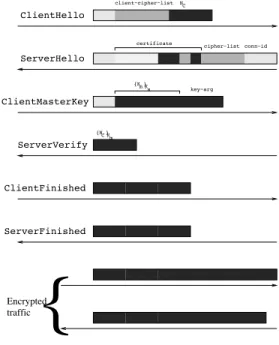
(i.e., n = 256). NC Ks {K }m Km Encrypted traffic {N }C ClientFinished ServerVerify ServerFinished
{
ClientHello ServerHello ClientMasterKey client−cipher−list conn−id certificate cipher−list key−argFigure 1: Normal SSL v2 Session
Encrypted traffic is (using state-of-the-art crypto-graphic algorithms) indistinguishable from random traf-fic. The byte entropy of a random sequence of charac-ters is 8 bits per byte, at least in the limit N → +∞. On the other hand, the byte entropy of a non-encrypted sequence of characters is much lower. According to [5, Section 6.4], the byte entropy of English text is no greater than 2.8, and even 0-order approximations do not exceed 4.26.
Let us convey the idea of using byte entropy to de-tect attacks. For example, the mod_ssl attack [16] uses a heap overflow vulnerability during the key exchange (handshake) phase of SSL v2 to execute arbitrary code on the target machine. A normal (simplified) execution of this protocol is tentatively pictured in Figure 1. Flow direction is pictured by arrows, from left (client) to right (server) or conversely. The order of messages is from top to bottom. The handshake phase consists of the top six messages. Encrypted traffic then follows. We have given an indication of the relative level of entropy by levels of shading, from light (clear text, low entropy) to dark gray (encrypted traffic, random numbers, high entropy).
Hijacked traffic
{
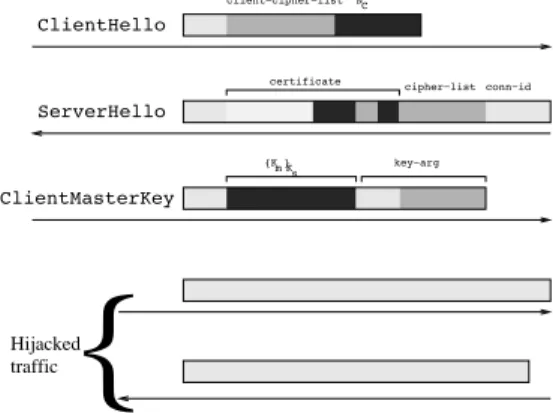
NC Ks {K }m ClientHello ServerHello ClientMasterKey client−cipher−list conn−id certificate cipher−list key−argFigure 2: Hijacked SSL v2 Session
Shell codes that are generally used with the mod_ssl attack hijack one session, and reuse the https connection to offer basic terminal facilities to the remote attacker. We detect this by realizing that the byte entropy of the flow on this connection, which should quickly approach 8, remains low. See Figure 2 for an illustration of what this should look like. Note that, since the shell code com-municates in clear after the key exchange phase, entropy will be low in the bottom messages. (The last three mes-sages of the handshake have been skipped by the shell code. Note that, since they are encrypted, there is no way to distinguish them from post-handshake encrypted traffic.) In fact, since the shell code itself, whose entropy is low, is sent in lieu of a session key, the entropy is al-ready low in some parts of the key exchange. This can be used to detect the attack even if the shell code does not communicate over the https channel, which is also common.
Just the same method applies to detect the SSH CRC32 attack [39], or more recent attacks that subvert traffic that ought to be encrypted, or random, or com-pressed under normal conditions of use. (See examples in Section 7.3)
Outline. We start by reviewing related work in Sec-tion 2. This will be an opportunity for us to review al-ternate detection mechanisms, and to state the known limitations of each approach (including ours). We then introduce the notion of sample entropy and its proper-ties in Section 3. We show in Section 4 how the sample entropy can be evaluated, and used to give reliable esti-mators of whether a given piece of traffic is scrambled (encrypted, compressed, random) or not. In particular, we shall see that the sample entropy is capable of esti-mating this on very short bursts of characters with high confidence. We briefly review other possible estimators of disorder in Section 5. In Section 6, we examine how this can be put to use in detecting attacks, where only parts of the protocol messages are meant to be scram-bled, and may be subverted—as in Figure 2. We describe how we implemented this in theNet-Entropy sensor, see Section 7. Finally, we conclude in Section 8.
2 Related Work
Entropy and sample entropy have been standard notions in statistics since the pioneering work of C. E. Shan-non [28]. They have been used in countless works. We shall review related work on sample entropy and entropy estimators, as needed, in the next section, where we view basic notions and some required mathematical re-sults.
In security, the idea of using the sample entropy to collect some statistical information about a network has already been used, e.g., in [10]. However, our purpose is different. We do not attempt to detect information about a network (e.g., detecting what a user types from timing delays between keystrokes over SSH [29]), rather we wish to detect typical attacker behavior. The entropy of data has already been used as heuristic in virus and malware detection: most of common binary executable files have an average entropy around 6.5 (depending of the compiler, processor architecture, operating system, binary file format). Malicious software executables are usually packed, compressed and/or encrypted. This op-eration increases the entropy of files. An entropy analy-sis phase is included in the PEiD tool [12]. Data entropy has also been included into file system forensic analy-sis tools such as WinHex Forensic [37], which need to guess the type of files on given file systems (low entropy files are text, XML, mails, binary files; high entropy files are multimedia, compressed, encrypted files). Our focus is different, and the idea of detecting subverted crypto-graphic protocols, i.e., instances where scrambled flow is expected but clear text is found, is new. We shall see that some of the problems that crop up in this setting re-quire new solutions, e.g., see Section 6.
verifica-tion of cryptographic protocols (see e.g. [11] for an entry point). These works are concerned with verifying certain properties such as secrecy, or authentication on idealized models of communication. Our point here is to analyze actual network flows. In particular, we consider distribu-tions of characters in these flows, which is out of reach of the aforementioned methods.
Next, let us investigate what other methods are avail-able to detect subverted cryptographic protocols, and in general how attacks such as [16] or [39] can be detected today.
Snort [26] detects these attacks by comparing all flows against signatures for known shellcodes and traffic they generate. This is reasonable, because shellcodes will ap-pear in clear during the attack phase, and because only a few dozen standard shellcodes are routinely used in cur-rent exploits. (This is very similar to virus detection.) It therefore suffices to list a few characteristic byte se-quences, corresponding to each particular shellcode. One problem with this approach is that the signature base has to be maintained, and enriched each time a new shellcode or attack appears on the hacking scene.
Our approach, on the contrary, applies independently of the actual shellcode used, and applies to zero-day at-tacks. This is also the case for PAYL [33], where worms are detected by evaluating a so-called Manhattan dis-tance between reference one-character distributions and observed traffic. Other possible distances include the Mahanobis distance [34]. One could also argue for the
Kullback-Leibler distance [5], which in general lends
it-self to more rigorous mathematical argumentation. Our use of the sample entropy can be seen as a special case of this distance, where the reference distribution is uniform. Naturally, there is no silver bullet, and every detection technique can be countered. To counter ours, it would suffice for an attacker to use a relatively small shellcode that encrypts its own communication, or even does not communicate at all on the monitored ports, and whose binary code is itself scrambled (i.e., encrypted, or com-pressed, namely whose binary code achieves a high en-tropy). Technology to scramble binary code can be taken from the world of encrypted, polymorphic, or metamor-phic viruses [31]. It is therefore possible to defeat our mechanism—at least in principle; we shall see in Sec-tion 4.2 that our mechanism is so sensitive that it is in fact able to tell polymorphic shellcodes apart from en-crypted traffic.
Another countermeasure against cryptographic proto-col subversion is to check that all key exchanges are properly formatted. E.g., in the mod_ssl attack [16], the ClientMasterKey message (3rd message in the handshake) will hold a key_arg field of the wrong size. If the intruder detection system is able to monitor each protocol, and recompute all sizes on the fly, this would be
a way of detecting these attacks. This is rather complex, and we shall argue against it in Section 6.1. Computing entropies is also much simpler.
3 Sample Entropy and Estimators
First, a note on notation. Recall that we take log to de-note base 2 logarithms. Entropies will be computed us-ing log, and will be measured in bits. The notation ln is reserved to natural logarithms. Some papers we shall refer to use natural logarithms. We shall then adapt their results without mentioning it explicitly; this will usually involve introducing a factor 1/ ln 2 = log e ∼ 1.4427.
Let w be a word of length N, over an alphabet Σ =
{0, 1, . . . , m − 1}. We may count the number niof oc-currences of each letter i ∈ Σ. The frequency fiof i in
wis then ni/N. The sample entropy of w is: ˆ
HNM LE(w) = − m−1"
i=0
filog fi
(The superscript MLE is for maximum likelihood
esti-mator.) If w is a random word over Σ, where each
char-acter is drawn uniformly and independently, the frequen-cies fiwill tend to 1/m in probability as N tends to in-finity, by the law of large numbers.
The formula is close enough to the notion of entropy of a random source, but the two should not be confused. Given a probability distribution p = (pi)i∈Σover Σ, the
entropy of p is
H(p) = −
m"−1
i=0
pilog pi
In the case where each character is drawn uniformly and independently, pi= 1/m for every i, and H(p) = log m.
It is hard not to confuse H and ˆHM LE
N , in particular because a property known as the asymptotic equiparti-tion property (AEP, [5, Chapter 3]) states that, indeed,
ˆ
HM LE
N (w) converges in probability to H(p) when the length N of w tends to +∞, as soon as each character of
wis drawn independently according to the distribution p. In the case of the uniform distribution, this means that
ˆ
HM LE
N (w) tends to log m. When characters are bytes,
m = 256, so ˆHM LE
N (w) tends to 8 (bits per byte). Before we continue, note that the approximation ˆ
HM LE
N (w) ∼ H(p) is valid when N & m.
However, we are not interested in the limit of ˆ
HM LE
N (w) when N tends to infinity. There are several reasons for this. First, actual messages we have to mon-itor may be of bounded length. E.g., the encrypted pay-load may be only a few dozen bytes long (N ≤ 100, whereas m = 256) in short-lived SSH connections. Sec-ond, even though we may count on N being large for
some encrypted connections, we have to decide at some
time point whether traffic is scrambled or not: we use
a cutoff, typically N ≤ 216 = 65 536, and will only
compute the entropy of the first 65 536 bytes of traffic. Third, it is important to detect intrusions at the earliest time possible. If we can detect unscrambled traffic after just a few dozen bytes, we should emit an alert, and take countermeasures, right away.
0 1 2 3 4 5 6 7 8 1 4 16 64 256 1024 4096 16384 65536
Entropy (bits per byte)
Data size (bytes)
Statistical Entropy log2(N)
Figure 3: Average Sample Entropy ˆHM LE
N (w) of Words
wof Size N
Let us plot the average ˆHM LE
N of ˆHNM LE(w) when w is drawn uniformly among words of size N, for m = 256, and N ranging from 1 to 65 536 (Figure 3). Please note that the x-axis has logarithmic, not linear scale. ( ˆHM LE
N was evaluated by sampling over words gener-ated using the /dev/urandom source.) The value of
H(p)is shown as the horizontal line y = 8. As the-ory predicts, when N & m, typically when N is of the order of roughly at least 10 times as large as m, then ˆHM LE
N ∼ H(p). On the other hand, when N is small (roughly at least 10 times as small as m), then
ˆ
HM LE
N ∼ log N. Considering the orders of magnitude of N and m cited above, clearly we are interested in the regions where N ∼ m. . . precisely where ˆHM LE
N is far from H(p).
At this point, let us ask ourselves what the state of the art is in this domain. The field of research most con-nected to this work is called entropy estimation [2], and the fact that N ∼ m or N < m is often characterized as the fact that the probability p is undersampled. In classi-cal statistics, our problem is often described as follows. Take objects that can be classified into m bins (our bins are just bytes) according to some probability distribution
p. Now take N samples, and try to decide whether the entropy of p is log m (or, in general, the entropy of a given, fixed probability distribution) just by looking at the samples. The papers [1, 23, 24] are particularly rele-vant to our work, since they attempt to achieve this pre-cisely when the probability is undersampled, as in our case.
The problem that Paninski tries to solve [23, 24] is finding an estimator ˆHN of H(p), that is, a statis-tical quantity, computed over randomly generated N-character words, which gives some information about the value of H(p). Particularly interesting estimators are the
unbiased estimators, that is those such that E( ˆHN) =
H(p), where E denotes mathematical expectation (i.e., the average of all ˆHN(w) over all N-character words w). If we have an unbiased estimator ˆHN of H(p), then our detection problem is easy: compute ˆHN over the
N-character input word w, then if ˆHN(w) = 8 up to some small tolerance ! > 0, then w is random enough (hence almost certainly scrambled), otherwise w is un-scrambled. Because we reason up to !, we may even tolerate a small bias; the bias of ˆHN is E( ˆHN) − H(p).
The sample entropy ˆHM LE
N , introduced above, is an estimator, sometimes called the plug-in estimate, or
max-imum likelihood estimator [23]. As Figure 3
demon-strates, it is biased, and the bias can in fact be rather large. So ˆHM LE
N does not fit our requirements for ˆHN. Let us say right away that, while the limit N → +∞ of the estimator ˆHM LE
N is unbiased, a surprising result due to Antos and Kontoyiannis is that the error between an estimator of H(p) and H(p) converges to 0 arbitrarily slowly, when p is arbitrary: see [1, Theorem 4], or [23, Section 3.2]. In a sense, this means that finding an unbi-ased estimator of the actual entropy of the flow is diffi-cult. However, our problem is less demanding: we only want to distinguish this actual entropy from the entropy of the uniform distribution U.
0 1 2 3 4 5 6 7 8 1 4 16 64 256 1024 4096 16384 65536
Average entropy (in bit per Bytes)
Data size (in Byte)
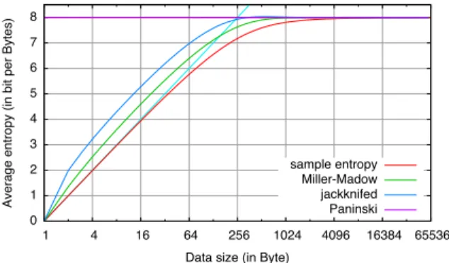
sample entropy Miller-Madow jackknifed Paninski
Figure 4: Sample Entropy Estimators Comparing ˆHM LE
N to the entropy at the limit, log m, is wrong, because ˆHM LE
N is biased for any fixed N. Nonetheless, we may introduce a correction to the es-timator ˆHM LE
N . To this end, we must estimate the bias. Historically, the first estimation of the bias is the Miller-Madow bias correction [19] ( ˆm− 1)/(2N ln 2), where
ˆ
m = |{i|fi (= 0}| is the number of characters that do appear at all in our N-character string w, yielding the
Miller-Madow estimator: ˆ HM M N (w) = HˆNM LE(w) + ˆ m− 1 2N ln 2 = − m"−1 i=0 filog fi+ ˆ m− 1 2N ln 2 Another one is the jackknifed MLE [8]:
ˆ HNJK(w) = N ˆHNM LE(w) − N− 1 N N " j=1 ˆ HNM LE(w−j)
where w−jdenotes the (N − 1)-character word obtained from w by removing the jth character. While all these corrected estimators indeed correct the 1/N term from biases at the limit N → +∞, they are still far from being unbiased when N is small: see Figure 4.
In the case that interests us here, i.e., when p if the uniform distribution over m characters, an exact asymp-totic formula for the bias is known as a function of c > 0 when N and m both tend to infinity and N/m tends to c [23, Theorem 3]. (See also Appendix A.) The corrected estimator is: ˆ HP N(w) = HˆNM LE(w) − log c (1) +e−c +∞ " j=1 cj−1 (j − 1)!log j
While the formula is exact only when N and m both grow to infinity, in practice m = 256 is large enough for this formula to be relevant. On our experiments, the difference between the average of ˆHP
N(w) over random experiments and log m = 8 is between −0.0002 and 0.0051 for N ≤ 100 000, and tends to 0 as N tends to infinity. (On Figure 4, it is impossible to distinguish
ˆ
HNP—the “Paninski” curve—from 8.) We can in partic-ular estimate that ˆHP
N is a reasonably unbiased estimator of H(p), when p is the uniform distribution.
4 Evaluating the Average Sample Entropy
Instead of trying to compute a correct estimator of the actual entropy H(p), which is, as we have seen, a rather difficult problem, we turn the problem around.
Let HN(p) be the N-truncated entropy of the distri-bution p = (pi)i∈Σ. This is defined as the average of the sample entropy ˆHM LE
N (w) over all words w of length N, drawn at random according to p. In other words, this is what we plotted in Figure 3. A direct summation shows
that HN(p) = " n0,...,nm−1∈N n0+...+nm−1=N #$ N n0, . . . , nm−1 % pn0 0 . . . p nm−1 m−1 × &m−1 " i=0 −nNilognNi ' ( where $ N n0, . . . , nm−1 % = N ! n0! . . . nm−1! is the multinomial coefficient.
When p is the uniform distribution U (where pi = 1/m for all i), we obtain the formula
HN(U) = 1 mN " n0,...,nm−1∈N n0+...+nm−1=N #$ N n0, . . . , nm−1 % × (2) &m"−1 i=0 −nNi lognNi ' (
By construction, ˆHNM LEis then an unbiased estimator of HN. Our strategy to detect unscrambled text is then to take the flow w, of length N, to compute ˆHM LE
N (w), and to compare it to HN(U). If the two quantities are significantly apart, then w is not random. Otherwise, we may assume that w looks random enough so that w is likely to be scrambled.
Not only is this easier to achieve than estimating the actual entropy H(p), we shall see (Section 4.2) that this provides us much narrower confidence intervals, that is, much more precise estimates of non-randomness.
For example, if w is the word
0x55 0x89 0xe5 0x83 0xec 0x58 0x83 0xe4 0xf0 0xb8 0x00 0x00 0x00 0x00 0x29 0xc4 0xc7 0x45 0xf4 0x00 0x00 0x00 0x00 0x83 0xec 0x04 0xff 0x35 0x60 0x99 0x04 0x08
of length N = 32 (which is much less than m = 256), then ˆHM LE
N (w) = 3.97641, while HN(U) = 4.87816, to 5 decimal places. Since 3.97641 is significantly less than 4.87816 (about 1 bit less information), one is tempted to conclude that w above is not scrambled. (This is indeed true: this w is the first 32 bytes of the code of the main() function of an ELF executable, compiled under gcc. However, we cannot yet conclude, until we compute confidence intervals, see Section 4.2.)
Consider, on the other hand, the word
0x85 0x01 0x0e 0x03 0xe9 0x48 0x33 0xdf 0xb8 0xad 0x52 0x64 0x10 0x03 0xfe 0x21 0xb0 0xdd 0x30 0xeb 0x5c 0x1b 0x25 0xe7 0x35 0x4e 0x05 0x11 0xc7 0x24 0x88 0x4a
This has sample entropy ˆHN(w) = 4.93750. This is close enough to HN(U) = 4.87816 that we may want to conclude that this w is close to random. And indeed, this
wis the first 32 bytes of a text message encrypted with
gpg. Comparatively, the entropy of the first 32 bytes of the corresponding plaintext is only 3.96814.
Note that, provided a deviation of roughly 1 bit from the predicted value HN(U) is significant, the ˆHNM LE estimator allows us to detect deviations from random-looking messages extremely quickly: using just 32 char-acters in the examples above. Actual message sizes in SSL or SSH are of the order of a few kilobytes.
4.1 Computing H
N(
U)
There are basically three ways to compute HN(U). (Re-call that we need this quantity to compare ˆHM LE
N (w) to.) The first is to use Equation (2). However, this quickly becomes unmanageable as m and N grow. Indeed, the outer summation is taken over all m-tuples of integers that sum to N, of which there are exactly)N +m−1
m−1 *
. For
m = 2, this would be an easy sum of N + 1 terms. For
m = 256, this would mean summing O(N255) terms.
E.g., for a 1 kilobyte message (N = 1 024), this would amount to 2635, or about 10191terms.
0 0.0005 0.001 0.0015 0.002 0.0025 0.003 0.0035 0.004 0.0045 1 4 16 64 256 1024 4096 16384 65536
Average error (in bit per Bytes)
Data size (in Byte) Figure 5: Error Term in (3)
A much better solution is to recall Equation (1). An-other way of reading it is to say that, for each constant c, when N and m tend to infinity in such a way that N/m is about c, then HN(U) = log m (3) + log c − e−c +∞ " j=1 cj−1 (j − 1)!log j + o(1) As we have seen, when m = 256, this approxima-tion should give a good approximaapproxima-tion of HN(U). In fact, this approximation is surprisingly close to the ac-tual value of HN(U). The o(1) error term is plotted in
0 500 1000 1500 2000 2500 3000 3500 4000 4500 5000 0 500 1000 1500 2000 2500 3000 3500 4000 # Iterations c 1.09*x+240
Figure 6: Number of Iterations to Convergence (96-Bit Floats)
Figure 5. It is never more than 0.004 bit, and decreases quickly as N grows.
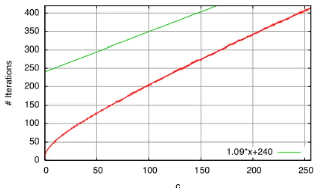
The above series converges quickly. The series is a sum of positive numbers, so that rounding errors tend not to accumulate. We have implemented this series us-ing 96-bit IEEE floatus-ing-point numbers, by summus-ing all terms until the sum stabilizes (i.e., until the next term is negligible compared to the current partial sum, yield-ing results precise to about 51–63 bits of mantissa). The number of iterations needed is roughly linear in c, see Figure 6. Note that we have gone as far as c = 4 000, corresponding to N = 1 024 000. This would only be needed for connections lasting for about 1 Mb. In prac-tice, with a cutoff of 64 Kb, we never need more than 415 iterations, see Figure 7.
0 50 100 150 200 250 300 350 400 0 50 100 150 200 250 # Iterations c 1.09*x+240
Figure 7: Number of Iterations to Convergence (96-Bit Floats)
On a 1.6 GHz Pentium-M laptop, computing all values of this function from 0.001 to 128 by steps of 0.001 takes 2.65 s., i.e., each computation of the series takes 21µs. on average. (Recall that we compute this series up to roughly 51 bits, i.e., 18 decimal digits, although we only really need 4 or 5 digits.) Depending on the context, this may be fast enough or not. If this is not fast enough, tabulating all the values of the function from 1/256 ∼
0.004 to 128 by steps of 0.004 requires us to store 384Kb of data, using 96 bit floats, or just 128Kb using 32 bit floats (which is enough for the precision we need).
The third method to evaluate HN(U) is the stan-dard Monte-Carlo method consisting in drawing enough words w of length N at random, and taking the average of ˆHN(w) over all these words w. This is how we eval-uated HN(U) in Figure 3, and how we defined the refer-ence value of HN(U) which we compared to (3) in Fig-ure 5. To be precise, we took the average over 100 000 samples for N < 65 536, taking all values of N below 16, taken one value in 2 below 32, one value in 4 be-low 64, . . . , and one value in 4 096 bebe-low 65 536. The spikes are statistical variations that one may attribute to randomness in the source. Note that they are in general smaller than the error term o(1) in (3).
We can then compute HN(U) by this Monte-Carlo method, and fill in tables with all required values of
HN(U) (note that m is fixed). While this is likely to use only about 128Kb already, we can save some memory by exploiting the fact that HN(U) is a smooth and increas-ing [23, Proposition 3] function of c, by only storincreas-ing a few well-chosen points and extrapolating; and by using the fact that values of c that are not multiples of 4/256 or even 8/256 are hardly ever needed.
In the sequel, and in particular in Section 6, we shall need to evaluate more complicated functions, notably functions of which we know no asymptotic approxima-tion such as (3). We shall always compute them by look-ing up tables, filled in by such Monte-Carlo methods.
4.2 Confidence Intervals
Evaluating ˆHM LE
N (w) only gives a statistical indication of how close we are to HN(U). Recall our first exam-ple, where w was the first 32 bytes of the code of the main()function of some ELF executable. We found
ˆ
HM LE
N (w) = 3.97641, while HN(U) = 4.87816. What is the actual probability that w of length N = 32 is un-scrambled when ˆHM LE
N (w) = 3.97641 and HN(U) = 4.87816?
It is again time to turn to the literature. Ac-cording to [1, Section 4.1], when N tends to +∞,
ˆ
HM LE
N is asymptotically Gaussian, in the sense that
√
N ln 2( ˆHM LE
N − H) tends to a Gaussian distribution with mean 0 and variance σ2
N = V ar{− log p(X)}. In non-degenerate cases (i.e., when σ2
N > 0), the expecta-tion of ( ˆHM LE
N − H)2is Θ(1/N). . . but precisely, the
p =U case is degenerate.
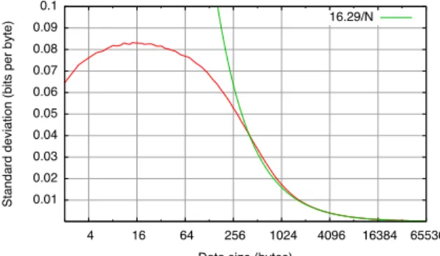
As we have already said, our interest is not in the limit of large values of N. Unfortunately, much less is known about the variance of ˆHM LE
N = ˆHNM LE when N ∼ m or N < m than about its bias. One useful inequality is that the variance of ˆHM LE
N is bounded from above by
log2
N/N[1, Remark (iv)], but this is extremely
conser-vative. 0.01 0.02 0.03 0.04 0.05 0.06 0.07 0.08 0.09 0.1 4 16 64 256 1024 4096 16384 65536
Standard deviation (bits per byte)
Data size (bytes)
16.29/N
Figure 8: Standard Deviation of ˆHM LE
N (w) 0.00024 0.00049 0.00098 0.002 0.0039 0.0078 0.016 0.031 0.062 0.13 4 16 64 256 1024 4096 16384 65536
Standard deviation (bits per byte)
Data size (bytes)
16.29/N
Figure 9: Standard Deviation of ˆHM LE
N (w), in Log Scale
On the other hand, we may estimate the standard deviation of ˆHN by a Monte-Carlo method, estimat-ing the statistical standard deviation SD( ˆHM LE
N ) of ˆ
HM LE
N (w), on random words w of length N. The re-sult is shown as the thick curve in Figure 8. It turns out that SD( ˆHNM LE) evolves as 16.29/N when N → +∞, as Figure 9 (y-axis in logarithmic scale) makes clear. The coefficient 16.29 here is+m−1
2 1
ln 2: as predicted
by [20, Equation (12)], the variance of ˆHM LE
N evolves as σ2
N + 2Nm−12ln22 when N → +∞, and in our case
σ2
N = 0, as we have seen. SD( ˆHNM LE) reaches its max-imum (about 0.08 bit) for N of the order of 16, while for
N ≥ m the standard deviation is so close to 16.29/N
that we can equate the two for all practical purposes. In particular, for typical packet sizes of 1, 2, 4, and 8 Kb, the standard deviation SD( ˆHM LE
N ) is 0.016, 0.008, 0.004, and 0.002 bit respectively. This is small.
Then, we can also estimate percentiles, again by a Monte-Carlo method, see Figure 10: the y values are given so that a proportion of all words w tested falls within y × SD( ˆHM LE
0 0.5 1 1.5 2 2.5 3 3.5 4 1 4 16 64 256 1024 4096 16384 65536
Confidence interval (SD units)
Data size (bytes) 99.9% 99% 95% 90% 75% 50% Figure 10: Percentiles ˆ HM LE
N . The proportions go from 50% (bottom) to 99.9% (top). Note that, unless N ≤ 16 (which is unre-alistic), our estimate of ˆHM LE
N is exact with an error of at most 4SD( ˆHM LE
N ), with probability 99.9%, and that 4SD( ˆHN) is at most 64/N, and in any case no larger than 0.32 bit (for words of about 16 characters).
Let’s return to our introductory question: What is the actual probability that w of length N = 32 is un-scrambled when ˆHM LE
N (w) = 3.97641 and HN(U) = 4.87816? For N = 32, SD( ˆHNM LE) is about maximal, and equal to 0.081156. So we are at least 99.9% sure that the entropy of a 32-byte word with characters drawn uni-formly is 4.87816 ± 4 × 0.081156, i.e., between 4.55353 and 5.20279: if ˆHM LE
N (w) = 3.97641, we can safely bet that w is not scrambled. Note that N = 32 is almost the worst possible case we could dream of. Still, ˆHM LE
N is already a reliable estimator of randomness here.
For packets of sizes 1, 2, 4, and 8 Kb, and a confidence level of 99.9% again, ˆHM LE
N is precise up to ±0.0625,
±0.0313, ±0.0156, and ±0.0078 bit respectively.
Data source Entropy
(bits/byte) ˆ
HM LE
N HN
Binary executable (elf-i386) 6.35 8.00
Shell scripts 5.54 8.00 Terminal activity 4.98 8.00 1 Gbyte e-mail 6.12 8.00 1Kb X.509 certificate (PEM) 5.81 7.80 ± 0.061 700b X.509 certificate (DER) 6.89 7.70 ± 0.089 130b bind shellcode 5.07 6.56 ± 0.24 38b standard shellcode 4.78 5.10 ± 0.28 73b polymorphic shellcode 5.69 5.92 ± 0.27 Random 1 byte NOPs (i386) 5.71 7.99 Figure 11: Sample Entropy of Some Common Non-Random Sources
We report some practical experiments in Figure 11,
on non-cryptographic sources. This gives an idea of the amount of redundancy in common data sources. The entropy of binary executables (ELF format, i386 archi-tecture) was evaluated under Linux and FreeBSD by collecting all .text sections of all files in /bin and /usr/bin. Similarly, the entropy of shell scripts was computed by collecting all shell scripts on the root vol-ume of Linux and FreeBSD machines (detected by the file command). Terminal activity was collected by monitoring a dozen telnet connections (port 23) on tcpfrom a given machine with various activity, such as text editing, manual reading, program compilation and execution (about 1 Mb of data). As far as e-mail is con-cerned, the measured entropy corresponds to 3 years of e-mail on the first author’s account. These correspond to large volumes of data (large N), so that HN is 8 to 2 decimal places, and confidence intervals are ridiculously small.
The next experiments were made on smaller pieces of data. Accordingly, we have given HNin the form H ±δ, where δ is the 99.9% confidence interval. Note that X.509 certificates are definitely classified as unscram-bled. We have also tested a few shellcodes, because, first, as we have seen in Figure 1 and Figure 2, it is in-teresting to detect when some scrambled piece of data is replaced by a shellcode, and second, because detect-ing shellcodes this way is challengdetect-ing. Indeed, shell-codes are typically short, so that HN is significantly dif-ferent from 8. More importantly, modern polymorphic and metamorphic virus technologies, adapted to shell-codes, make them look more scrambled. (In fact, the one we use is encrypted, except for a very short pro-log.) While the first two shellcodes in Figure 11 are correctly classified as unscrambled (even a very short 38 byte non-polymorphic shellcode), the last, polymor-phic shellcode is harder to detect. The 99.9% confidence interval for being scrambled is [5.65, 6.19]: the sample entropy of the 73 byte polymorphic shellcode is at the left end of this interval. The 99% confidence interval is 5.92 ± 0.19, i.e., [5.73, 6.11]: with 99% confidence, this shellcode is correctly classified as non-scrambled. In practice, shellcodes are usually preceded with padding, typically long sequences of the letter A or the hexadec-imal value 0x90 (the No-OPeration i386 instruction), which makes the entropy decrease drastically, so the ex-amples above are a worst-case scenario. Detecting that the random key-arg field of Figure 1 was replaced by a shellcode in Figure 2 is therefore feasible.
Another worst-case scenario in polymorphic viruses and shellcodes is given by mutation, whereby some spe-cific instructions, such as nop, are replaced with other instructions with the same effect, at random. This fools pattern-matching detection engines, and also increases entropy. However, as the last line shows on a large
amount of random substitutes for nop on the i386 ar-chitecture, this makes the sample entropy culminate at a rather low value compared to 8.
We conclude this section by noting that ˆHM LE N is a re-markably precise estimator of HN(U), even in very un-dersampled cases.
5 Other Estimators of Randomness
We have chosen to estimate the entropy H(p) of an un-known distribution p to detect whether p is close to the uniform distribution or not. While this works well in practice, there are other ways to evaluate randomness: see [13, Section 3.3], or [21].
For example, we may check that the mean!m−1 i=0 ifi is close to (m − 1)/2. (Recall that fi = ni/N is the frequency of letter i.) We may check that the χ2statistic
ˆ VN(w) = m"−1 i=0 (ni− Npi)2 N pi = m"−1 i=0 (ni− N/m)2 N/m
(when pi= 1/m is the uniform distribution U) is not too large. Recall [13, Section 3.3.1.C] that, in the limit N → +∞, the probability that ˆVN(w) ≤ v, for any v > 0, tends to the χ2function with m − 1 degrees of freedom.
It is also well-known that, in this case, and letting ν =
m− 1, then ˆVN(w) is less than ν +
√
2νxπ+ 2/3x2π− 2/3 + O(1/√ν) with probability π, where xπ = 1.64 for π = 0.95, say, and m > 30 [13, Section 3.3.1.A]. Let us just note that ˆVN(w) should be of the order of m − 1 when p = U, and N → +∞.
One may think of computing all, or at least some of these quantities, to get an improved test of randomness. However, here is an informal argument that suggests that this would be pointless. To simplify things, assume that
Nis large (recall that the χ2approximation is only valid
for large N).
If the sample entropy ˆH(w)is close to its maximum
value log m (when p = U), it is known that the frequen-cies fiare close to 1/m, say fi = 1/m + δi. Since the derivative of −x log x is − log x−1/ ln 2, and its second derivative is −1/(x ln 2), we may approximate ˆH(w)by
ˆ H(w) = log m + m"−1 i=0 δi(log m − 1/ ln 2) − m"−1 i=0 m δ 2 i 2 ln 2 + o &m"−1 i=0 δi3 '
The first sum vanishes, since!m−1
i=0 δi= 0. So ˆ H(w)− log m = − m 2 ln 2 m−1" i=0 δi2+ o &m−1 " i=0 δi3 ' Since ni− N/m = Nδi, ˆVN(w) = mN !m−1i=0 δ2i, so ˆ H(w)− log m = − 1 2N ln 2VˆN(w) + o &m−1 " i=0 δ3 i '
With probability π = 0.95, ˆVN(w) will be of the order of
ν = m− 1, and we retrieve a form of the Miller-Madow
estimator: ˆH(w)−log m is roughly −(m−1)/(2N ln 2)
when p = U. In other words, a χ2 test essentially
amounts to estimating the Miller-Madow bias correction, and checking that it is small. This is only valid in the limit N → +∞, and we estimated the bias much more precisely in Section 3 anyway.
We also note that Fu et al. [10] compared empirically the sample mean, sample variance, and sample entropy as indicators of randomness, and observed that of the three, sample entropy was the most robust, i.e., the least sensitive to noise.
There are many other statistical tests. One weakness of tests based on sample entropy is that ˆHN(w) depends only on the frequencies fi. Any permutation of the let-ters in w would give rise to the same sample entropy. In particular, ˆHN(w) is unable to note the difference be-tween the regular sequence of letters 0, 1, . . . , m − 1, 0, 1, . . . , m − 1, 0, . . . , and a truly random one. (To be fair, it will detect a difference for small N, where ˆHN will rise more slowly on the regular sequence.) Testing the average, or a χ2statistic, suffers from the same
prob-lem. Some other tests, such as the serial test or the gap test [13, Section 3.3.2], or Maurer’s universal statistical test [14], or compression tests [5, Chapter 5], do not, and are able to detect correlations between letters. The de-fect that most of them share is that they require large data volumes, i.e., large values of N, to be significant. In fact, variants of the entropy test also do detect corre-lations between letters, as first shown by Shannon [28]: just compute the entropy of digraphs (pairs of letters at positions i, i + 1), trigraphs (letters at positions i, i + 1,
i + 2), for example.
We have chosen not to investigate this. While this in-deed improves our estimate of randomness, the simple sample byte entropy ˆHN(w), with m = 256, was enough in practice. Furthermore, computing the latter can be done by maintaining an array of 256 values of −filog fi over each connection. This is relatively straightforward to implement, and uses small computing resources. On the other hand, computing the entropy of digraphs re-quires up to 65 536 entries per array, which may clog the machine. It is imaginable that computing the entropy of consecutive nibble pairs would offer some advantage here. (A nibble is a half-byte; and no, the entropy of nib-ble digraphs is not the same as the byte entropy, because of byte-straddling pairs of nibbles).
6 Taking into Account Unscrambled
Sec-tions
Until now, we have explored a sweetened situation, where we had one word (a packet, a flow of charac-ters during a connection, say), and we wanted to decide whether it was scrambled or not, as a whole. Referring to our coloring conventions of Figure 1 and Figure 2, this allows us to detect whether observed traffic is all dark gray, or contains enough light gray spots.
However, as we can see on Figure 1—and although colors were exaggerated—, some sections of the ob-served traffic have to be light gray. In typical crypto-graphic protocols, at least some of the first messages ex-changed are in clear, and not random. We should not conclude that an attack is in progress here.
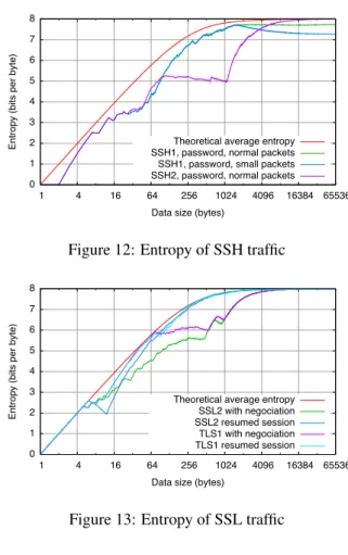
Moreover, some specific protocols insert a more or less important bias. The ideal case of a cryptographic protocol over TCP would exhibit only encrypted traffic. This is what SSH2 does, for example. Other protocols add some control information in clear to encrypted pack-ets. This adds a bias to the entropy estimator, which may or may not be negligible. A case in point is the binary packet format for SSH1 (seen at the TCP level), which starts with the packet length in clear (4 bytes), then contains 1 through 8 padding bytes (usually pseudo-random), and finally the encrypted SSH1 packet. The most significant bytes of the 4-byte packet length field will be zero most of the time. (In practice, TCP pack-ets are no longer than a few kilobytes.) Over a full SSH1 connection spanning several TCP packets, the sample en-tropy will therefore tend to a value smaller than 8, de-pending on distribution of packet lengths. In our expe-rience, we routinely observed limiting values of around 7.95: see Figure 12, in particular the two SSH1 curves. One particular concern is that this bias is in effect con-trolled by the untrusted client user, who may force the SSH1 client to send identical-sized packets: it suffices for the client to send the same message over and over, e.g., using a shell script. The extreme case is that of a client typing an e-mail message, where each typed letter gives rise to a 1-byte packet, followed by an echo 1-byte packet.
The same problem occurs in the TLS protocol: each TLS record begins with a content type identifier (1 byte, 0x17for application data, 0x15 for alerts, etc.), the ver-sion of the protocol (two fixed bytes, 0x0301 in the case of TLS 1.0), the record length (2 bytes), and finally the encrypted payload.
The above examples show that entropy may be lower than expected. In other cases, the entropy can also be higher than expected. A typical example is when coun-ters or sequence numbers are encountered in clear, which re-increases entropy, compared to constant data such as
version numbers or type identifiers.
This incurs two problems. First, we should use the ˆ
HM LE
N estimator to detect whether some specific, not all, sections of traffic are scrambled (dark gray, high en-tropy). These specific sections are dependent on the pro-tocol used. If some of these specific sections has low entropy (light gray), an alert is reported. To this end, we may track connections, and compute the sample entropy of various sections of traffic, depending on the port on which communication takes place (e.g., 443 for https). We explore how this can be done for known protocols, such as SSL, in Section 6.1. We shall see that this ap-proach is unrealistic. We describe simpler and more re-alistic approaches in Section 6.2 and Section 6.3.
The second problem is that the intuition of coloring that we used in Figure 1 and Figure 2 is meaningless, at least formally. There is no such thing as the sample entropy at a given byte in the flow. The concept of en-tropy only makes sense on words (or subwords) of suf-ficient length. Fortunately, as we have seen in previous sections, we only need to explore rather short subwords to get a reliable enough estimate of scrambledness.
6.1 Known Protocols
For well-known cryptographic protocols such as SSH (port 22), or SSL—including https (port 443), nntps (563), ldaps (636), telnets (992), imaps (993), ircs(994), pop3s (995), smtps (465)—, it is fea-sible to document which parts of traffic should have high entropy.
Most if not all of these protocols start with a key ex-change, or handshake, phase, usually followed by en-crypted traffic. The most critical sections are found in this initial handshake phase. Once keys have been es-tablished, there is no practical way to break the protocol. (We do not consider attacks which use the protocol with-out breaking it, such as the SUN login-over-SSH buffer overflow exploit [7].) It seems therefore particularly im-portant that sample entropies are estimated precisely dur-ing the handshake phase.
If all sections are of fixed size, this is easy to do. E.g., on the example of Figure 1, compute ˆHM LE
N (w) on the topmost dark subword NCof the ClientHello mes-sage (NC is 16 bytes long, about the worst-case as far as confidence intervals are concerned, but as we have seen, sample entropy can already be estimated accu-rately in this case); then compute it on the light-and-dark certificate subword of the ServerHello mes-sage when it arrives, and so on. Provided that these sub-words are large enough, this will provide us a reliable estimate whether these sections are scrambled or not.
Note that the certificate subword is not uni-formly light or dark. This is because this is an X.509
certificate, with some data in clear (light), and some en-crypted signatures (dark). We should therefore also parse X.509 certificates, and only compare the entropy of those parts of the certificate that contain scrambled data (typi-cally signatures).
In general, however, sections are of varying sizes. For example, in SSL versions 2 and up, key sizes are them-selves subject to negociation between client and server during the handshake phase. Some fields are optional: in the ClientHello message of Figure 1, an optional session ID field can be inserted before the NC field in case of session resumption. X.509 certificates may have varying sizes, depending on the number of fields filled in, on the sizes of clear text descriptions of issuers, cer-tificate authorities, etc.
In other words, to implement this solution, we need to implement a full parser for the protocol at hand (e.g., SSL), together with parsers for X.509 certificates and other fields of varying size and structure. This is done anyway in products such as Ethereal [4]. The only sim-ple way we know of doing this is to include standard code that does it. E.g., in the SSL case, we may just import relevant code from the OpenSSL project [22]. But the complete implementation of a new protocol parser may introduce more security flaws than using an already ma-ture library. A vivid illustration of this principle was re-cently produced when it was discovered that the Snort intrusion detection system [26] was remotely vulnerable through its Back Orifice protocol parser [17].
In general, the approach sketched here, of embedding a full parser for the protocols at hand, has a major draw-back: any buffer overflow attack on the original library (e.g., OpenSSL) will be present in the entropy monitor-ing tool. . . and will be triggered in exactly the same situations. The need for maintaining code as standards evolve is also a drawback of this approach.
We must therefore conclude that the approach of pars-ing known protocols completely is unrealistic.
6.2 Aggregating Fields
Instead, we shall aggregate fields, or even whole mes-sages. In other words, we shall compute the sample en-tropy of fields or messages as a whole. For example, the X.509 certificate of the ServerHello message of Fig-ure 1 is expected to have an overall entropy of roughly 6.89, according to Figure 11.
Naturally, aggregating fields means that confidence in-tervals must be made wider. In the current state of the art, it seems that no mathematical theory is available to pre-dict the actual mean and variance of ˆHM LE
N on whole fields or messages, similarly to the results of previous sections. We shall however give an idea how ˆHM LE
N evolves when we switch from one light to one dark area
0 1 2 3 4 5 6 7 8 1 4 16 64 256 1024 4096 16384 65536
Entropy (bits per byte)
Data size (bytes)
Theoretical average entropy SSH1, password, normal packets SSH1, password, small packets SSH2, password, normal packets
Figure 12: Entropy of SSH traffic
0 1 2 3 4 5 6 7 8 1 4 16 64 256 1024 4096 16384 65536
Entropy (bits per byte)
Data size (bytes)
Theoretical average entropy SSL2 with negociation SSL2 resumed session TLS1 with negociation TLS1 resumed session
Figure 13: Entropy of SSL traffic in the next section.
6.3 Bumps
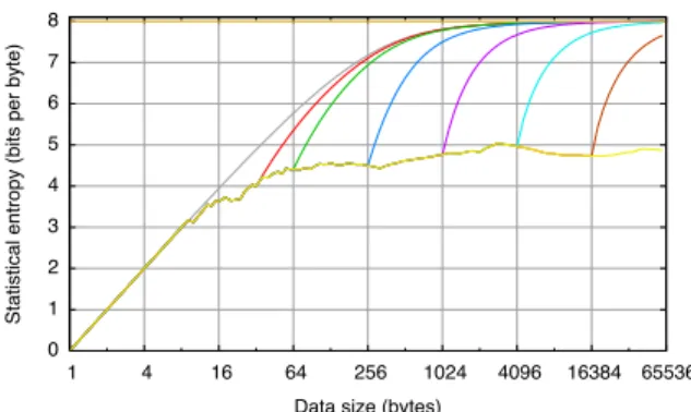
To give an idea how ˆHM LE
N evolves when several fields of different entropies are concatenated, we illustrate this on random messages of length N, with a prefix of length
N1generated using a low entropy source, say of entropy
H1; followed by a high-entropy suffix, say with source
entropy equal to H2. Actual messages naturally exhibit
a more complex mix of zones, but our point here is to make clearer what curves should be expected on simple examples.
Asymptotic formulae for this case are not too hard to obtain, but are rather obscure. Making statistical exper-iments and plotting the resulting curves is far more in-structive. We plotted ˆHM LE
N for varying values of N from 0 to 65 535, and for varying values of N1(32, 64,
256, 1 024, 4 096, and 16 384) in Figure 14. This rep-resents what should be expected from messages with a Base64 encoded prefix of length N1 followed by a
se-quence of scrambled bytes.
While we only see the low-entropy prefix, i.e., for the first N1bytes, the sample entropy follows the usual curve
for ˆHM LE
N1 , which we have already discussed at length,
0 1 2 3 4 5 6 7 8 1 4 16 64 256 1024 4096 16384 65536
Statistical entropy (bits per byte)
Data size (bytes)
Figure 14: Switching From Random Base64 to Random Characters
our experiment). After the N1first characters, we see a
sharp increase in entropy, connecting the first curve to a similar-shaped curve whose new limit is H2(8 bits in our
experiment).
It is only to be expected that any switch from one field to another field of differing entropies will then be observ-able as a sharp turn in direction, either upwards (going to a higher-entropy field) or downwards (exiting a high-entropy field).
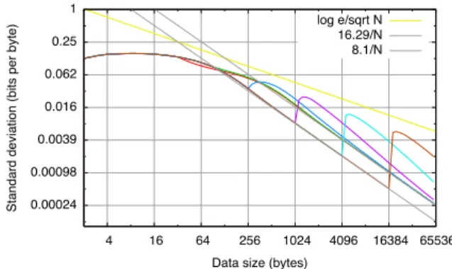
More interesting is the standard deviation obtained this way. This is plotted in Figure 15, together with two ref-erence straight lines. The 16.29/N line is the asymptotic standard deviation for the sample entropy of the high-entropy source. The standard deviation for the low en-tropy source would be aligned on a lower line, of y-value 8.10/N. (Remember the formula is+m−1
2 1 ln 2 N; for
Base64 encoding, m ∼ 6, yielding 8.10/N.) This fig-ure reads as follows. While we are looking at the low-entropy prefix, the standard deviation is as low as pre-dicted in earlier sections. Long after we have entered the high-entropy suffix, the standard deviation progressively approaches its asymptote 16.29/N—a very low value. The new effect here is that the standard deviation jumps to higher values just after we have switched from one field to the next.
This might be detrimental to the quality of the esti-mation. However, notice that the top of the bump, for each value of N1, always remains below the log e/
√ N
line. Remember that, in non-degenerate cases (i.e., when
σ2
N > 0), the expectation of ( ˆHNM LE− H)2is Θ(1/N) (Section 4.2), i.e., that, up to a 1/ ln 2 factor to make up for our use of base-2 logarithms, the standard deviation in non-degenerate cases is of the order Θ(1/√N ).
Re-member also that the steady-state behavior, i.e., on long fields with the same source entropy, is degenerate.
In other words, the standard deviation is low (Θ(1/N)) on long enough sequence of bytes with the same entropy, and goes up to about Θ(1/√N )when we
switch from one field to another with different source en-tropy.
This is bad news in a sense, because one consequence is that confidence intervals will necessarily be larger than in the simple cases studied before Section 6. But ob-serve that the actual bit values are low anyway. On Fig-ure 15, the standard deviation never exceeds 0.15 bits globally (as in previous experiments), and the standard deviation at the highest point in the bump after N1 is
0.046 bit (reached after 352 bytes, when N1 = 256),
resp. 0.024 bit (reached after 1 280 bytes, when N1 =
1 024), resp. 0.0116 bit (reached after 5 120 bytes, when
N1 = 4 096), resp. 0.0056 bit (reached after 20 480
bytes, when N1 = 16 384). Remember that 99.9%
per-centiles were at about 3.5 times the standard deviation around the average. This corresponds to 99.9% confi-dence intervals of ±0.161, resp. ±0.084, resp. ±0.041, resp. ±0.020 bit around the average.
0.00024 0.00098 0.0039 0.016 0.062 0.25 1 4 16 64 256 1024 4096 16384 65536
Standard deviation (bits per byte)
Data size (bytes)
log e/sqrt N 16.29/N 8.1/N
Figure 15: Standard Deviation (Base64 + Random) We conducted a similar experiment when the low-entropy prefix (the first N1 bytes) was not a random
Base64 file, but rather the first N1bytes of a given text—
namely the TEX source of the paper [27]. The results are shown in Figure 16 and Figure 17. While the curves are slightly different, we are forced to reach the same con-clusions: going from one field to the next forces a sharp jump in the sample entropy, and grows small bumps into the standard deviation curve.
In other words, to detect abnormal values of the sam-ple entropy, confidence intervals should not be an issue. But the expected shapes of entropy curves should show some sharp jumps at some specific positions in the in-coming flow. These positions are not entirely known. However, we can classify areas in the plane where the sample entropy is representative of normal behavior. For example, Figure 18 shows 5 398 valid connections, plus one attack, which were observed from real traffic at LSV. Every valid connection falls into a series of rectangu-lar areas. Note that valid connections produce varying curves, depending on protocol version and actual
0 1 2 3 4 5 6 7 8 1 4 16 64 256 1024 4096 16384 65536
Statistical entropy (bits per byte)
Data size (bytes)
Figure 16: Switching From Given Text to Random Char-acters 0.00024 0.00098 0.0039 0.016 0.062 0.25 1 4 16 64 256 1024 4096 16384 65536
Standard deviation (bits per byte)
Data size (bytes)
log e/log N 16.29/N
Figure 17: Standard Deviation (Text + Random)
mentation of the protocol. They can all be classified by the displayed sequence of rectangles. Observe also that the unique attack shown here exhibits a sharp differ-ence from the curves, and exits the rectangular areas fast. We only represent the sample entropy of the whole con-nection, but measured on a per-packet basis. The attack curve exits after the 6th packet (1 939 cumulated bytes), in a clear way. 1 2 3 4 5 6 7 8 16 64 256 1024 4096 16384 65536
Entropy (bits per byte)
Data size (bytes)
Authorized SSH attack
Figure 18: SSH Normal Behavior, and an Attack
7 Implementation in the Net-Entropy
Sen-sor
Net-entropy is a user program (not a kernel module) written in C. We use the pcap library [32] to implement low-level network frame capture, and the LibNIDS li-brary [35, 36] to implement IP defragmentation and TCP stream reassembly. The latter library is a user-land port of the Linux TCP/IP stack (kernel 2.0.36).
While this seems simple enough, there is a catch. We have observed that, in certain situations, LibNIDS incor-rectly classified sniffed packets as invalid. This is not a problem with LibNIDS. Instead, this is a side-effect of modern implementations of TCP/IP stacks. E.g., kernels will not compute packet checksums on machines with re-cent network interface cards, which implement hardware acceleration feature (TCP segmentation offload, hard-ware Rx/Tx checksumming). In other words, the kernel relies on the network interface card to compute check-sums in hardware, and just sets these checkcheck-sums to zero. But then, any sensor that captures network flow while running on one peer of the connection will get packets from the local loop, i.e., with zero checksums, and these will appear to be invalid. This is totally inconsequential ifNet-entropy runs on a router, which is the intended application, since the router is never one of the peers. In caseNet-entropy were to be used directly on a work-station, we would need to get around this, typically by adding a special case to the LibNIDS checksum verifica-tion routine, to ignore invalid checksums in data coming
Port: 22
Direction: both Cumulative: yes RangeUnit: bytes
# Range: start end min_ent max_ent Range: 1 63 0 4.38105154 Range: 64 127 4.22877741 4.64838314 Range: 128 255 4.95194340 5.02499151 Range: 256 511 4.86894369 7.28671360 Range: 512 1023 4.86310673 7.59574795 Range: 1024 1535 4.94409609 7.74570751 Range: 1536 2047 5.77497149 7.81915951 Range: 2048 3071 6.44314718 7.85139179 Range: 3072 4095 7.17234325 7.92034960 Range: 4096 8191 7.46498394 7.96606302 Range: 8192 65536 7.82608652 7.99687433 Figure 19: An example range file, for SSH (port 22) from the local host.
TheNet-entropy sensor keeps track of all connections of configured protocols and emits an alarm via the Unix
Syslog system when sample entropy is out of specified
bounds. Net-Entropy was designed to run on routers or intrusion detection hosts, by passively sniffing the net-work.
For performance reasons,Net-entropy limits the anal-ysis to the first 64 Kb of data in network connections. We also drop connection monitoring after some predefined timeout. Indeed, it may happen that the sensor misses the termination of the connection, for example in cases of network or CPU overload. It is also well-known that limiting monitoring processes is good practice. In par-ticular, this avoids attacks where the malicious attacker starts many simultaneous connections, e.g., testing for passwords, without terminating them properly (with a TCP FIN or RST packet). A timeout is used to get rid of these dead connections. This timeout is set by de-fault to 15 minutes (900 seconds). Every connection that has remained inactive for this long will be removed from monitoring. This behavior makesNet-entropy more re-sistant to denial-of-service and brute force attacks (SYN flood, SSH scan).
Let us recall that we want to check key exchanges, not user activity. It is extremely unlikely that a key exchange take any longer than a few seconds, even on low band-width networks. Note that a delayed key exchange is abnormal, whatever its entropy.
7.1 Configuring Net-Entropy
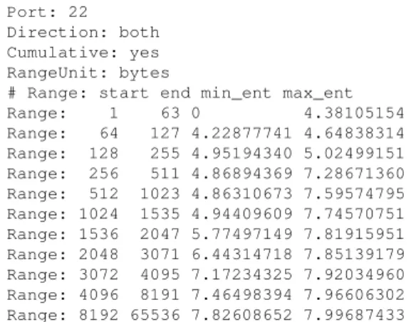
As already hinted at the end of Section 6.3,Net-entropy checks the sample entropy of monitored connections on specified ranges. Configuring these ranges is done through protocol-specific range files. Figure 19 shows an example of a range file, for the SSH protocol (port 22).
Looking directly at the Range: lines, one observes that ranges are specified as rectangular areas. E.g., the first row states that, for SSH connections, the sample en-tropy between the first byte and byte number 63 should be between 0 and 4.38105154. Size ranges, e.g., from byte 1 to byte 63, are specified here in byte units, but can also be specified on a per-packet basis, by replac-ing the bytes keyword in the RangeUnit: line by packets.
It would be a hassle if the user of Net-entropy had to include all these information by hand. Instead, we provide a supervised learning mode where the user only specifies size ranges, andNet-entropy fills out the least and highest entropy values, from either a live network capture or from a libpcap capture file.
Each range file contains a definition for one protocol exactly. As the example above shows, we identify pro-tocols by their server ports, at the TCP destination. For-mally, a range file consists of a list of dirlist directives, obeying the following grammar:
dirlist: dirlist directive | directive yesno: “yes” | “no”
direction: “cli2srv” | “srv2cli” | “both” rangeunit: “bytes” | “packets”
directive: “Port:” INT
| “Direction:” direction | “Cumulative:” yesno | “RangeUnit:” rangeunit | “Range:” INT INT FLOAT FLOAT where INT stands for a positive integer (included in [1, +∞)) and FLOAT for a rational number (included in [0, 8]). Empty lines and lines beginning with a ‘#’ are silently ignored.
A range file must contain a port number and at least one range. The Direction directive allows one to choose which data to analyze, depending on the direc-tion of the TCP flow. Possible direcdirec-tions are cli2srv for analyzing only data from client to server, srv2cli for server to client only and both for all data. The de-fault value is both, in case this directive is omitted.
The default value of the Cumulative directive is yes, meaning that statistical entropy will be computed on a per-connection basis, periodically checking whether it is in the indicated valid ranges. If the Cumulative directive is set to no, statistical entropy will be computed for each packet separately, restarting from zero at each packet boundary.
As we said earlier, the RangeUnit: directive the unit in which size ranges are measured. It is either packetsor bytes (default).
The Range: directive allows one to define a new range. It takes four parameters. The first two denote the size range, the other two are the least and highest al-lowed entropies for this range. Net-entropy does a few consistency checks, e.g., that entropies are between 0 and
8, that the highest entropy for a range n1–n2is at most
log n2, that size ranges do not overlap, and are sorted in
increasing order.
Entropy fields can be left empty, by writing an IEEE 754 NaN (Not a Number) in the corresponding field. This is taken as an indication by the supervised learn-ing mode that the range file should be updated. Uslearn-ing the -l option toNet-entropy will then modify the range file and fill out the required entropy fields. Additionally, using Net-entropy with the -l option will replace en-tropy alerts by mere update messages.
To avoid congestion, the range file is only updated once a connection is terminated for which some entropy bound has to be modified. In particular, this means that trainingNet-entropy through an interactive SSH session won’t change the range file, until the user quits the ses-sion.
As is customary in every anomaly detection technique, it is important to trust the learning set, otherwise the pro-tocol ranges will be wrong or biased. Tools such as Ethe-real [4] allow one to select packets from network cap-ture files very precisely, and to edit capcap-tures so as to re-move offending outliers before sending the training data toNet-entropy with options -l, and -r (offline cap-ture).
The command line options ofNet-Entropy are sum-marized in the following table:
Parameter Arg Default value Interface -i <if> First interface Off-line file -r <file> No file Packet capture filter -f <filter> No filter
Runtime user -u <user> root Memory limit -m <lim> No limit Connection data size limit -t <lim> 65536 bytes
Connection timeout -T <timeout> 900 seconds Rule file -P <file> No rule Learning mode -l Disabled Erase old range file -d Disabled
Change config file -c net-entropy .conf Statistics files -s <dir> No statistics Flush statistics -F Disabled Per-byte statistics -b Per packet Net-entropy is also configured through the use of a system-wide configuration file, organized as a list
paramlist of parameters. The configuration file format
is defined by the following grammar: paramlist: paramlist param | param
param: “Interface:” STRING | “PcapFilter:” STRING | “RuntimeUser:” STRING | “MemoryLimit:” INT | “MaxTrackSize:” INT | “ConnectionTimeout:” INT | “ProtoSpec:” STRING
where INT stands for a positive integer and STRING for a character string. The Interface parameter, as well
as the -i option, allows one to choose the network in-terface used for the capture. If this parameter is omit-ted, the first available network interface reported by the operating system is used. The PcapFilter param-eter (-f option) is the filter used by the pcap library. The RuntimeUser parameter (-r) sets the user ac-count name which will be used for dropping root priv-ileges, e.g. the pcap or nobody users, or a dedicated system account. (Net-entropy is meant to start up as root, if only to allow network capture to function prop-erly.) The MemoryLimit parameter (-m) sets the maxi-mum memory limit that theNet-entropy sensor can use. This limit is a security against denial of service (DoS) attacks. The MaxTrackSize parameter (-t) sets the number of bytes after which a connection will cease to be monitored. The ConnectionTimeout parameter (-T) is the delay after which connections will be as-sumed to be inactive, and their monitoring will cease. The ProtoSpec parameter (-P) adds range files for ad-ditional protocols to be monitored.
The performance of the Net-entropy sensor can be significantly enhanced when BSD Packet Filters [15] are used in the libpcap. The point is that protocols which we are not interested in will simply be ignored at the ker-nel level. For example, it is meaningful to monitor SSH connections coming from outside a local area network (LAN), so as to detect intrusions on the LAN. It is less in-teresting to monitor outgoing SSH connections. Another case where BSD packet filters are useful is when Net-entropy is deployed on a router for some LAN, but we know that only a few machines on the LAN implement a given protocol (e.g., https will only run on secured servers on the LAN). In this case, BSD packet filters can be used to focus on packets on given ports and given ad-dresses or sub-networks. This can be done with a filter of the form:
(dst net LAN and
(dst port port1 or ... or dst port portn)) or
(src net LAN and
(src port port1 or ... or src port portn))
where LAN is the address of the network to protect, and
portn are TCP ports of protocols to protect. This ba-sic filter template works on a common network. More complex filters should be used depending of the network structure to protect.
7.2 Net-Entropy Alert Messages
Net-entropy emits different kinds of alerts. We illustrate this on Figure 20, which exhibits a fictitious connection that generates all kinds of alerts. Alerts can be emitted during a connection:
• Entropy alarm start: entropy is below the
![Figure 21: Net-Entropy Limits with mod ssl Attack The second demonstration attack [39] exploits a bug in SSH servers](https://thumb-eu.123doks.com/thumbv2/123doknet/12395461.331577/19.918.483.803.418.612/figure-entropy-limits-attack-second-demonstration-exploits-servers.webp)
