HAL Id: inria-00363593
https://hal.inria.fr/inria-00363593
Submitted on 23 Feb 2009
HAL is a multi-disciplinary open access
archive for the deposit and dissemination of
sci-entific research documents, whether they are
pub-lished or not. The documents may come from
teaching and research institutions in France or
abroad, or from public or private research centers.
L’archive ouverte pluridisciplinaire HAL, est
destinée au dépôt et à la diffusion de documents
scientifiques de niveau recherche, publiés ou non,
émanant des établissements d’enseignement et de
recherche français ou étrangers, des laboratoires
publics ou privés.
Software
Peggy Cellier, Mireille Ducassé, Sébastien Ferré, Olivier Ridoux
To cite this version:
Peggy Cellier, Mireille Ducassé, Sébastien Ferré, Olivier Ridoux. Formal Concept analysis enhances
Fault Localization in Software. Int. Conf. Formal Concept Analysis, 2008, Montreal, Canada. pp.273–
288. �inria-00363593�
Fault Localization in Software
Peggy Cellier1 2, Mireille Ducass´e2, S´ebastien Ferr´e1, and Olivier Ridoux1
1 IRISA/University of Rennes 1,2IRISA/INSA de Rennes,
[email protected], http://www.irisa.fr/LIS/
Abstract. Recent work in fault localization crosschecks traces of cor-rect and failing execution traces. The implicit underlying technique is to search for association rules which indicate that executing a particular source line will cause the whole execution to fail. This technique, how-ever, has limitations. In this article, we first propose to consider more expressive association rules where several lines imply failure. We then propose to use Formal Concept Analysis (FCA) to analyze the resulting numerous rules in order to improve the readability of the information contained in the rules. The main contribution of this article is to show that applying two data mining techniques, association rules and FCA, produces better results than existing fault localization techniques.
1
Introduction
The execution of a program in a testing environment generates a set of data about the execution, called a trace of the execution. Traces allow the program to be monitored and permit the program to be debugged when some executions fail, namely produce unexpected results. A trace can contain different kinds of information, for example the executed lines, and the verdict of the execution (FAIL or PASS ). Fault localization often investigates the contents of traces to find the reasons of failures. There exist several approaches to crosscheck traces. Some are based on the differences between a passed execution and a failed execu-tion [RR03,CZ05]. Others use statistical indicators in order to rank lines of the program [JHS02,LNZ+05,LYF+05]. In particular, Jones et al. [JHS02] propose
to measure a kind of correlation between executing a given line and failing a test. Denmat et al. [DDR05] show that this is similar to search for a restricted form of association rules [AIS93,AS94] and that the restriction leads to limitations.
Searching for association rules is a known data mining task with a well-documented rationale. The knowledge context is represented by a set of trans-actions (objects) described by a set of items (attributes). Searching that context for association rules consists in searching for implications where the premise and the conclusion are sets of attributes. In order to measure the relevance of the computed rules, some statistical indicators are used, such as support, confidence, or lift. In the framework of association rules, the method of Jones et al. consists in searching for rules with only one line in their premise and only the attribute
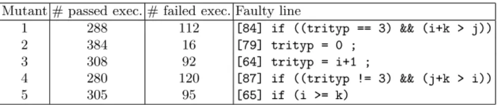
Mutant # passed exec. # failed exec. Faulty line
1 288 112 [84] if ((trityp == 3) && (i+k > j)) 2 384 16 [79] trityp = 0 ;
3 308 92 [64] trityp = i+1 ;
4 280 120 [87] if ((trityp != 3) && (j+k > i)) 5 305 95 [65] if (i >= k)
Table 1.Mutants of the Trityp program.
FAIL in conclusion. Note that the general association rule framework allows for several attributes in the premise.
Formal Concept Analysis (FCA) [GW99] has already been used for several software engineering tasks: to understand the complex structure of programs, in order to “refactor” class hierarchies for example [Sne05]; to design the class hierarchy of object-oriented software from specifications [GV05,AFHN06]; to find causal dependencies[Pfa06]. Tilley et al. [TCBE05] presented a survey on applications of FCA for software engineering activities : e.g. architectural design, software maintenance. FCA finds interesting clusters, called concepts, in data sets. The input of FCA is a formal context, i.e. a binary relation describing elements of a set of objects by subsets of properties (attributes). A formal concept is defined by a pair (extent, intent), where extent is the maximal set of objects that have in their description all attributes of intent, and intent is the maximal set of attributes common to the description of all objects of extent. The concepts of the context can be represented by a lattice where each concept is labelled by its intent and extent.
The main contribution of this article is to show that applying two data mining techniques, association rules and FCA, produces better results than existing fault localization techniques. This is discussed in detail Section 6. Another contribu-tion is to propose to build upon the intuicontribu-tion of existing methods: the difference or correlation between execution traces contains significant clues about the fault. We combine the expressiveness of association rules to search for possible causes of failure, and the power of FCA to explore the results of this analysis. The kind of association rules that we use allows some limitations of other methods to be alleviated. The goal of our method is no longer to highlight the faulty line but to produce an explanation of the failure thanks to the lattice.
In the sequel, Section 2 describes the running example used to illustrate the method. Section 3 presents the two contexts used by the method. Section 4 shows how to interpret the rule lattice in terms of fault localization. Section 5 discusses the statistical indicators. Section 6 presents the main contribution, the benefits of our method compared to other methods. Section 7 discusses further work.
2
Running Example
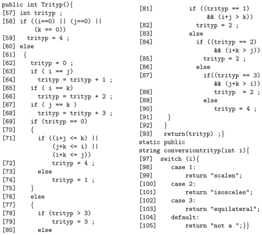
Throughout this article, we use the Trityp program given in Figure 1 to illustrate our method. It classifies sets of three segment lengths into four categories:
sca-public int Trityp(){ [57] int trityp ; [58] if ((i==0) || (j==0) || (k == 0)) [59] trityp = 4 ; [60] else [61] { [62] trityp = 0 ; [63] if ( i == j) [64] trityp = trityp + 1 ; [65] if ( i == k) [66] trityp = trityp + 2 ; [67] if ( j == k ) [68] trityp = trityp + 3 ; [69] if (trityp == 0) [70] { [71] if ((i+j <= k) || (j+k <= i) || (i+k <= j)) [72] trityp = 4 ; [73] else [74] trityp = 1 ; [75] } [76] else [77] { [78] if (trityp > 3) [79] trityp = 3 ; [80] else [81] if ((trityp == 1) && (i+j > k)) [82] trityp = 2 ; [83] else [84] if ((trityp == 2) && (i+k > j)) [85] trityp = 2 ; [86] else [87] if((trityp == 3) && (j+k > i)) [88] trityp = 2 ; [89] else [90] trityp = 4 ; [91] } [92] } [93] return(trityp) ;} static public
string conversiontrityp(int i){ [97] switch (i){ [98] case 1: [99] return "scalen"; [100] case 2: [101] return "isosceles"; [102] case 3: [103] return "equilateral"; [104] default: [105] return "not a ";}}
Fig. 1.Source code of the Trityp program.
lene, isosceles, equilateral, not a triangle. The program contains one class with 130 lines of code. It is a classical benchmark for test generation methods. Such a benchmark aims at evaluating the ability of a test generation method to detect errors by causing failure. To this purpose slight variants, mutants, of the bench-mark programs are created. The mutants can be found on the web1, and we use
them for evaluating our localization method. For the Trityp program, 400 test cases have been generated with the Uniform Selection of Feasible Paths method of Petit and Gotlieb [PG07]. Thanks to that method, all feasible execution paths are uniformly covered.
Table 1 presents the five mutants of the Trityp program that are used in this article. The first mutant is used to explain in details the method. For mutant 1, one fault has been introduced at Line 84. The condition (trityp == 2) is re-placed by (trityp == 3). That fault implies a failure in two cases. The first case is when trityp is equal to 2. That case is not taken into account as a particular
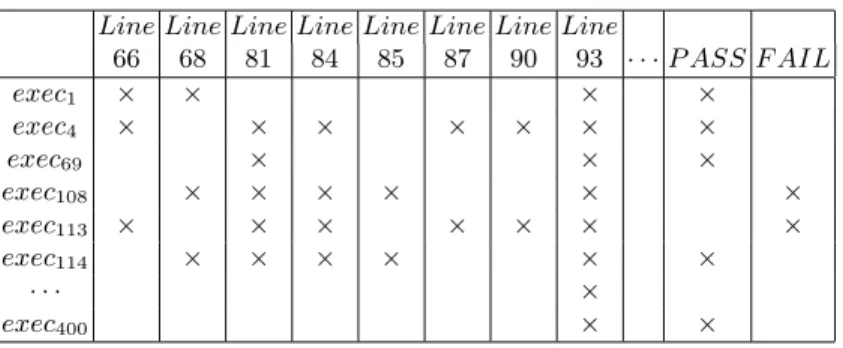
Line Line Line Line Line Line Line Line 66 68 81 84 85 87 90 93 · · · P ASS F AIL exec1 × × × × exec4 × × × × × × × exec69 × × × exec108 × × × × × × exec113 × × × × × × × exec114 × × × × × × · · · × exec400 × ×
Table 2.Example of the trace context for mutant 1 of the Trityp program.
case and thus treated as a default case, at Lines 89 and 90. The second case is when trityp is equal to 3. That case should lead to the test Line 87, but due to the fault it is first tested at line 84. Indeed, if the condition (i+k>j) holds, trityp is assigned to 2. However, (i+k>j) does not always entail (j+k>i), which is the real condition to test when trityp is equal to 3. Therefore, trityp is assigned to 2 whereas 4 is expected.
The fault of mutants 2 and 3 are on assignments. The fault of mutants 4 and 5 are on conditions.
3
Two Formal Contexts for Fault Localization
This section presents the information on which the localization process is based. Firstly, a context is built from execution traces, the trace context. Secondly, particular association rules are used to crosscheck the trace context. Thirdly, a second context is introduced in order to reason on the numerous rules, the rule context. How to interpret the rule lattice, associated to the rule context, is presented in Section 4.
The Trace Context. In order to reason about program executions we use traces of these executions. There are many types of trace information and discussing them is outside the scope of this article (see for example [HRS+00]). Let us only
assume that each trace contains at least the executed lines and the verdict of the execution, P ASS if the execution produces the expected results and F AIL otherwise. This is a common assumption in fault localization research. This forms the trace context. The objects of the trace context are the execution traces. The attributes are all the lines of the program and the two verdicts. Each trace is described by the executed lines and the verdict of the execution.
Table 2 gives a part of the resulting trace context for mutant 1. For instance, during the first execution, the program executes lines 66, 68, . . . and passes2.
Line Line Line Line Line Line Line Line Line Line Line Line 81 84 87 90 105 66 78 112 113 · · · 17 58 93 r1 × × × × × × × × × × × × r2 × × × × × × × × × × · · · r8 × × × × × × × r9 × × × × × ×
Table 3. Example of the rule context for mutant 1 of the Trityp program with minlif t= 1.25 and minsup = 1.
Association Rules. In order to understand the causes of the failed executions, we use a data mining algorithm [CFRD07] which searches for association rules. In addition, to reduce the number of association rules, we focus on association rules based on closed itemsets [PBTL99]. Namely, we search for association rules where 1) the premises are the intents of concepts whose extent mostly contains failed execution traces and few passed execution traces (according to the statistical indicators) and 2) the conclusion is the attribute F AIL (Definition 1). This corresponds to the selection of the concepts that are in relation with the concept labelled by F AIL. Note that those concepts can be in relation with the concept labelled by P ASS, too.
Definition 1 (association rules for fault localization). The computed as-sociation rules for fault localization have the form: L → F AIL where L is a set of executed lines such that L ∪ {F AIL} is the intent of a concept in the trace context and L ∩ {F AIL} = ∅.
Only the association rules that satisfy the minimum thresholds of the se-lected statistical indicators are generated. We have chosen the support and lift indicators. The support indicates the frequency at which the rule appears. In our application, it measures how frequently the lines that form the premise of a given rule are executed among the lines in a failure. The lift indicates if the occurrence of the premise increases the probability to observe the conclusion. Relevant rules are thus filtered with respect to a minimum support, minsup, and a minimum lift, minlif t. The threshold minsup can be very low, for in-stance to cope with failures that are difficult to detect (for details see Section 5). The threshold minlif t is always greater or equal to 1 because otherwise the lift indicates that the premises decrease the probability to observe the conclusion. The Rule Context. The computation of association rules generates a lot of rules, and especially rules with large premises. Understanding the links that exist between the rules, for example if a rule is more specific than another, is difficult to do by hand. The computed association rules, however, correspond to concepts of the trace context. They are partially ordered according to their premises; indeed L1 → F AIL is more specific than L2 → F AIL when L1and
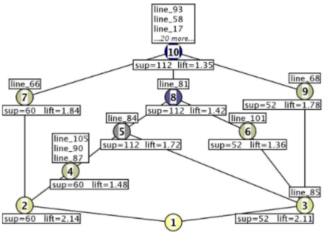
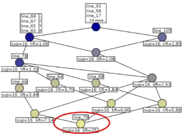
Fig. 2.Rule lattice for mutant 1 associated to the rule context of Table 3
rules, we propose to build a new context, the rule context. The objects are the association rules; the attributes are lines. Each association rules is described by the lines of its premise.
Table 3 shows a part of the rule context for mutant 1 of the Trityp program with the support threshold, minsup, equal to 1 object and the lift threshold minlif tequal to 1.25. The premise of rule1 contains : line 81, line 84, line 87,
line 90, . . .3In addition, line 78, line 112, line 113, . . ., line 17, line 58, line 93 are
present in all rules which means that they are executed by all failed executions.
4
A Rule Lattice for Fault Localization
The rule lattice is the concept lattice associated with the rule context. It allows association rules to be structured in a way that highlights the partial ordering which exists between them. Figure 2 displays the rule lattice associated with the rule context of Table 34. The remaining of this section presents a description of
the rule lattice and then gives an interpretation of it. 4.1 Description of the Rule Lattice
The rule lattice has the property that each concept can be labelled at most by one object. Indeed, two different rules cannot have the same premise. If, in the trace context, several executions have exactly the same description they are abstracted in a single rule in the rule context.
The rule lattice is presented in a reduced labelling. In that representation each attribute and each object is written only once. Namely, each concept is labelled by the attributes and the objects that are specific to it. It is the most widespread
3
Complete rule context: http://www.irisa.fr/LIS/cellier/icfca08/rules context.rl
representation. As a consequence, the premise of a rule r can be computed by collecting the attributes labelling all the concepts above the concept that is labelled by r [GW99]. For example, on Figure 2 the premise of the rule which labels Concept 3 is line 85, line 84, line 68, line 101, line 81, line 93, line 58, line 17, plus the other 20 attributes (lines) that label the top concept.
In the rule lattice, the more specific rules are close to the bottom. When the support threshold for searching for association rules is one object and the lift threshold is close to 1, each most specific rule represents a single execution path in the program that leads to a failure. For example, on Figure 2 there are two very specific rules, the two concepts closest to the bottom: Concept 2 and Concept 3. The rule which labels Concept 2 contains in its premise the lines 66, 105, 90, 87, 84, 81 and the label of the top concept. It corresponds to the failure case when trityp is equal to 2 (see Section 2). The rule which labels Concept 3 contains in its premise the lines 85, 84, 68, 101, 81 and the label of the top concept. It corresponds to the failure case when trityp is equal to 3 (see Section 2). By looking at the support value of each rule, we note that three rules relate to 60 failed executions (Concepts 2, 4, 7), in fact failed executions when trityp is equal to 2; three rules relate to 52 failed executions (Concepts 3, 6, 9), in fact failed executions when trityp is equal to 3; and three rules relate to 112 failed executions (Concepts 5, 8, 10), namely all failed executions. 4.2 Interpretation for Fault Localization
Navigating in the rule lattice bottom up first displays rules that are in general too specific to explain the error. It then displays rules that are more general and maybe more informative, and finally displays the top of the lattice which is la-belled by the attributes (line numbers) that are common to all failed executions. The bottom concept of the rule lattice in Figure 2 has no attribute in its labelling. During the debugging session two paths are proposed to follow. The leftmost path from the bottom concept, Concept 2, corresponds to the case where variable trityp is equal to 3 and condition (i+k>j) holds whereas the condition (j+k>i) does not hold. It leads to two concepts. The first concept is Concept 7 labelled by line 66, it is the statement which initializes trityp to 2. The second concept is Concept 4 labelled by three line numbers: 105, 90, 87. These lines correspond to the case when the variable trityp is equal to 2 and tritypis assigned to 4 when 2 is expected, i.e. the triangle is labelled as not a triangle instead of isosceles. Those two concepts are too specific but by looking at the rule of the concept upwards, the faulty line is localized. Concept 5 covers the greatest number of failed executions (support=112) and has the greatest lift among rules which have support equal to 112. The same reasoning can be done with the rightmost concept, Concept 3. It also leads to line 85. It corresponds to the then branch of the faulty conditional, i.e. the line where variable trityp is assigned to 2 when 4 is expected. The rule of that concept is too specific to understand the fault, it covers 52 failed executions. Following this path, three paths open upwards: two concepts whose rules have the same support as the rule of the concept that is labelled by line 85, Concept 6, 9; and a concept which
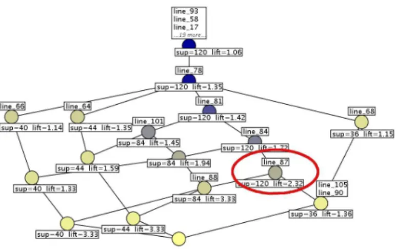
Fig. 3.Rule lattice from program Trityp with mutant 2 (faulty line 79) with minlift=1 and minsup=1.
Fig. 4. Rule lattice from program Trityp with mu-tant 3 (faulty line 64) with minlift=1 and minsup=1.
is labelled by line 84, the faulty line, Concept 5, whose rule covers the most number of failed executions (support=112).
This example shows that the rule lattice gives relevant clues for exploring the program. The faulty line is not highlighted immediately but exploring the lattice bottom up guides the user in its task to understand the fault.
4.3 More examples
One failed execution path. Figure 3 gives the rule lattice for mutant 2 when association rules are computed with minlif t=1 and minsup=1. Figure 4 gives the rule lattice for mutant 3 when association rules are computed with minlif t=1 and minsup=1. On those two examples the fault is a bad assignment. Only one execution path leads to a failure. We see in those cases that the faulty lines are immediatly highlighted in the label of the bottom concept. For example, in Figure 3 we see the faulty line 79 at the bottom. We remark that the dependencies between lines appear in the labelling. Indeed, in Figure 4 we see that the bottom concept is labelled not only by the faulty line 64 but also by line 79 and line 103. It is explained by two facts. Firstly, the execution of line 64 in a faulty way always implies the execution of line 79 and 103. Secondly, few executions that imply lines 64, 79 and 103 together pass. Note that all association rules of these examples have the same support. They cover all failed execution traces. Several failed execution paths. The execution of mutant 1 and 4 can fail with different execution paths. Mutant 1 was detailed in the previous section. Figure 5 gives the rule lattice for mutant 4 when association rules are computed with
Fig. 5.Rule lattice from program Trityp with mutant 4 (faulty line 87) with minlift=1 and minsup=1.
minlif t= 1 and minsup = 1. The fault of mutant 4 is at line 87. In the rule lattice of Figure 5, line 87 labels the concept which is labelled by a rule with the greatest support. In addition, among rules with the greatest support, this one has the greatest lift. In other words, line 87 is one of the common lines of all failed executions and with the least relation with passed executions.
Borderline case. Figure 6 gives the rule lattice for mutant 5 when association rules are computed with minlif t=1 and minsup=1. In the rule lattice, two failed execution paths are highlighted. One covers 33 of the failed executions. The other covers 62 of the failed executions. Looking at the common lines of those two execution paths, we find line 66. The associated rule of line 66 has the greatest lift among rules with support equal to 95. But the faulty line is 65. Line 65 labels the top concept of the rule lattice. The faulty line is thus not highlighted. It is due to the fact that line 65 is an if-statement executed by all executions. The number of failed executions that execute line 65 is thus very low with respect to the number of passed executions that execute line 65. However, line 66 is the then branch of the condition of line 65. The method does not highlight the faulty line but gives clues to find it.
5
Statistical Indicators
In order to compute and evaluate the relevance of association rules, several statistical indicators have been proposed, for example support, confidence, and lift [BMUT97]. The choice of statistical indicators and their thresholds is an
im-Fig. 6.Rule lattice from program Trityp with mutant 5 (faulty line 65) with min-lift=1 and minsup=1.
Fig. 7. Lattice from the rule context of mutant 1 with minlift=1.5 and min-sup=1.
portant part of the computation of association rules. Depending on the selected thresholds, the rule lattice may significantly vary and so does its interpretation. Typically, the support is the first filtering criterion for the extraction of as-sociation rules. It measures the frequency of a rule. For the fault localization problem, the value of minsup indicates the minimum number of failed execu-tions that should be covered by a concept of the trace context to be selected. Choosing a very high threshold, only the most frequent execution paths are rep-resented in the set of association rules. Choosing a very low threshold, minsup equals to one object, all execution paths that are stressed by the test cases are represented in the set of association rules. In our experiments, we choose minsup equals to one object. It is equivalent to search for all rules that cover at least one failed execution. The threshold can be greater in order to select less rules, but some failed execution paths would be lost, although in fault localization rare paths might be more relevant than common ones.
The other well-known indicator that we use is lift. In our approach, the lift indicates how the execution of a set of lines improves the probability to have a failed execution. The lift threshold can be seen as a resolution5 cursor. On
the one hand, if the threshold is high, few rules are computed, therefore few concepts appear in the lattice. It implies that the label of each concept contains a lot of lines, but each concept is very relevant. On the other hand, selecting a low threshold implies that more rules are computed. Those rules are less relevant and the number of concepts in the lattice increases. The number of attributes per label is thus reduced. For example, let us consider mutant 1 of program Trityp. Figure 2, already described in Section 4, shows the result lattice when the lift threshold is equal to 1.25. Figure 7 shows the result lattice when the lift threshold is equal to 1.5. Concept D of Figure 7 merges Concepts 5 and 8 of Figure 2. Concepts D and 5 actually correspond to the same rule. Concept 8 correspond to a more general rule with a lower lift. The same applies to Concepts C and 3, 6.
In addition, the concepts of the rule lattice have two properties thanks to the statistical indicators related to the trace lattice. Property 1 states that the support of rules that label the concepts of the rule lattice decreases when explor-ing the lattice top down. In the followexplor-ing, label(c)=r means that rule r labels concept c of the rule lattice. The extent of a set of attributes, X, is written ext(X), and kY k denotes the cardinal of set Y.
Property 1. Let c1 and c2 be two concepts of the rule lattice such that
label(c1)=r1 and label(c2)=r2. If c2< c1 then sup(r2) ≤ sup(r1).
Proof. The fact that c2 < c1 implies that the intent of c2 contains the
in-tent of c1. The intent of concept c1 (resp. c2) is the premise, p1 (resp. p2),
of rule r1 (resp. r2), thus p1 ⊂ p2. Conversely ext(p2) ⊂ ext(p1). As the
defini-tion of the support of a rule r = p → F AIL is sup(r) = kext(p) ∩ ext(F AIL)k, sup(r2) ≤ sup(r1) holds.
Property 2 is about the lift value. If two ordered concepts in the rule lattice are labelled by rules with the same support value, the lift value of the rule which labels the more specific concept is greater. That is why the rule lattice is explored bottom up (see Section 4.2).
Property 2. If c2< c1 and sup(r2) = sup(r1) then lif t(r2) > lif t(r1).
Proof. In the previous proof we have seen that c2 < c1 implies that ext(p2)
⊂ ext(p1). The definition of the lift of a rule r = p → F AIL is lif t(r) = sup(r)
kext(p)kkext(F AIL)k∗ kOk. As sup(r2) = sup(r1), and kext(p2)k < kext(p1)k,
lif t(r2) > lif t(r1) holds.
6
Benefits of Using Association Rules and FCA
The contexts and lattice structures introduced in the previous sections allow programmers to see all the differences between execution traces as well as all the differences between association rules. There exists other methods which compute differences between execution traces. Section 6.1 shows that the information about trace differences provided by our first context (and the corresponding lattice) is already more relevant than the information provided by four other methods proposed by Renieris and Reiss [RR03], as well as Zeller et al. [CZ05]. Section 6.2 shows that explicitly using association rules with several lines in the premise alleviate many of the limitations of Jones et al.’s method mentioned in the introduction [JHS02]. Section 6.3 shows that reasoning on the partial ordering given by the proposed rule lattice is more relevant than reasoning on total order rankings [JHS02,LNZ+05,LYF+05].
6.1 The Trace Context Structures Execution Traces
The first context that we have introduced, the trace context, contains the whole information about execution traces (see Section 3). In particular, the associated
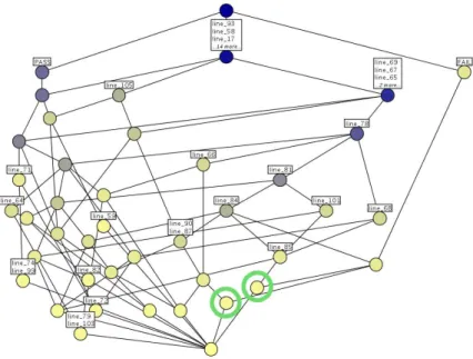
Fig. 8.Lattice from the trace context of mutant 1 of the Trityp program.
lattice, the trace lattice, allows programmers to see in one pass all differences between traces. Figure 8 shows the trace lattice of mutant 1.
There exists several fault localization methods based on the differences of execution traces. They all assume a single failed execution and several passed executions. We rephrase them in terms of search in a lattice to highlight their advantages, their hidden hypothesis and limitations.
The union model, proposed by Renieris and Reiss [RR03], aims at finding features that are specific to the failed execution. The method is based on trace differences between the failed execution f and a set of passed executions S: f − Ss∈Ss. The underlying intuition is that the failure is caused by lines that are executed only in the failed execution. Formalized in FCA terms, the concept of interest is the one whose label contains F AIL, and the computed information is the lines contained in the label. For example, in Figure 8 this corresponds to the upper concept on the right-hand side which contains no line in its label, namely the information provided by the union model is empty. The trace lattice presented in the figure is slightly different from the lattice that would be computed for the union model, because it represents more than one failed execution. Nevertheless, the union model often computes an empty information, namely each time the faulty line belongs to failed and passed execution traces. For example, a fault in a condition has a very slight chance to be localized. Our approach is based on the same intuition. However, as illustrated by Figures 8 and 2, the lattices that we propose do not lose information and help to navigate
in order to localize the faults, even when the faulty line belongs to failed and passed execution traces.
The union model helps localize bug when executing the faulty statement always implies an error, for example the bad assignment of a variable that is the result of the program. In that case, our lattice does also help, the faulty statement label the same concept as F AIL.
The intersection model [RR03] is the complementary of the previous model. It computes the features whose absence is discriminant of the failed execution: T
s∈Ss − f . Replacing F AIL by P ASS in the above discussion is relevant to
discuss the intersection model and leads to the same conclusions.
The nearest neighbor approach [RR03] computes the Ulam’s distance metrics between the failed execution trace and a set of passed execution traces. The computed trace difference involves the failed execution trace, f , and only one passed execution trace, the nearest one, p: f − p. That difference is meant to be the part of the code to explore. The approach can be formalized in FCA. Given a concept Cf whose intent contains F AIL, the nearest neighbor method
search for a concept Cp whose intent contains P ASS, such that the intent of Cp
shares as many lines as possible with the intent of Cf. On Figure 8 for example,
the two circled concepts are “near”, their share all their line attributes except the attributes F AIL and P ASS, therefore f = p and f − p = ∅. The rightmost concept fails whereas the leftmost one passes. As for the previous methods, it is a good approach when the execution of the faulty statement always involves an error. But as we see on the example, when the faulty statement can lead to both a passed and a failed execution, the method is not sufficient. In addition, we remark that there are possibly many concepts of interest, namely all the nearest neighbors of the concept which is labelled by F AIL. With a lattice that kind of behavior can be observed directly.
Note that in the trace lattice, the executions that execute the same lines are clustered in the label of a single concept. Executions that are near share a large part of their executed lines and label concepts that are neighbors in the lattice. There is therefore no reason to restrict the comparison to a single pass execution. Furthermore, all the nearest neighbors are naturally in the lattice.
Delta debugging, proposed by Zeller et al. [CZ05], reasons on the values of variables during executions rather than on executed lines. The trace information, and therefore the trace context, contains different types of attributes. Note that our approach does not depend on the type of attributes and would apply on traces containing other attributes than executed lines.
Delta debugging computes in a memory graph the differences between the failed execution trace and a single passed execution trace. By injecting the values of variables of the failed execution into variables of the passed execution, the method tries to determine a small set of suspicious variables. One of the purpose of that method is to find a passed execution relatively similar to the failed execution. It has the same drawbacks as the nearest neighbor method.
6.2 Association Rules Select a Part of the Trace Context
As it was presented in the introduction, Jones et al. [JHS02] compute association rules with only one line in the premises. Denmat et al. show that the method has limitations, because it assumes that an error has a single faulty statement origin, and lines are independent. In addition, they demonstrate that the ad hoc indicator which is used by Jones et al. is close to the lift indicator.
By using association rules with more expressive premises than the Jones et al. method (namely with several lines), the limitations mentioned above are alleviated. Firstly, the fault can be not only a single line, but the execution of several lines together. Secondly, the dependency between lines is taken into account. Indeed, dependent lines are clustered or ordered together.
The part of the trace context which is important to search for localizing a fault is the set of concepts that are around the concept labelled by F AIL; i.e. those that have a non-empty intersection with the concept labelled F AIL. Computing association rules with F AIL as a conclusion computes exactly those concepts, modulo the minsup and minlif t filtering. In other words the focus is done on the part of the lattice around the concept labelled by F AIL. For example, in the trace lattice of the Trityp program presented in Figure 8, the rule lattice when minlif t is very low (yet still attractive, i.e. minlif t>1), is drawn in bold lines.
6.3 The Rule Lattice Structures Association Rules
Jones et al.’s method presents the result of their analysis to the user as a coloring of the source code. A red-green gradient indicates the correlation with failure. Lines that are highly correlated with failure are colored in red, whereas lines that are highly not correlated are colored in green. Red lines typically represents more than 10% of the lines of the program, whithout identified links between them. Some other statistical methods [LNZ+05,LYF+05] also try to rank lines
in a total ordering. It can be seen as ordering the concepts of the rule lattice by the lift value of the rule in their label. From the concept ordering the lines in the label of those concepts can be ordered.
For example, on the rule lattice of Figure 2, the obtained ranking would be: line 85, line 66, line 68, line 84, . . . No link would be established between the execution of line 85 and line 68 for example.
The user who has to localize a fault in a program has a background knowledge about the program, and can use it to explore the rule lattice. The reading of the lattice gives a context of the fault and not just a sequence of independent lines to be examined, and reduces the number of lines to be examined at each step (concept) by structuring them.
7
Further work
The process proposed in this article for fault localization is already usable at the end of the debug session. When the programmer has a rough idea of the location
of the faults and that only a small part of the execution has to be traced, the current techniques to visualize lattices can be directly used.
However, we conjecture that the technique, with some extensions, can be used to analyze large executions. At present, the information is presented in terms of lines whereas it is not always the most relevant information granularity. For example, given a basic block (i.e. a sequence of instructions with neither branch-ing nor conditional), all its lines always appear in the same label. Displaybranch-ing the location of the basic block would be more relevant. This will help keeping concept labels to a readable size. We are currently working on the presentation of the results to reduce their size and to give more semantics to them so that they are more tractable for users.
Another further work is the computation of the concepts of the rule context directly from the trace context. Indeed, the concepts of the rule lattice belong to the trace lattice. However, gathering the two computations, association rules from the trace context and concepts from the rule context, is not a trivial task due to the statistical indicators which are not monotonous, for example the lift.
8
Conclusion
In this article we have proposed a new application of FCA: namely, fault localiza-tion. The process combines association rules and formal concept lattices to give a relevant way to navigate into the source code of faulty programs. Compared to existing methods, using a trace lattice has three advantages. Firstly, thanks to the capabilities of FCA to crosscheck data, our approach computes in one pass more information about execution differences than all the cited approaches together. In particular, the information computed by two methods, the union model and the intersection model, can be directly found in the trace lattice. Secondly, the lattice structure gives a better reasoning basis than any particular distance metrics to find similar execution traces. Indeed, all differences between the sets of executed lines of passed and failed executions are represented in the trace lattice. A given distance between two executions can be computed by dedi-cated reasoning on specific attributes. Thirdly, our approach treats several failed executions together, whereas the presented methods can analyze only one failed execution.
Moreover, the generality of the FCA framework makes it possible to handle traces that contain other information than lines numbers. In summary, cast-ing the fault localization problem in the FCA framework helps analyze existcast-ing approaches, as well as alleviate their limitations.
References
[AFHN06] G. Ar´evalo, J.R. Falleri, M. Huchard, and C. Nebut. Building abstractions in class models: Formal concept analysis in a model-driven approach. In Int. Conf. on MOdel Driven Engineering Languages and Systems, volume LNCS 4199, pages 513–527. Springer, 2006.
[AIS93] R. Agrawal, T. Imielinski, and A. N. Swami. Mining association rules be-tween sets of items in large databases. In P. Buneman and S. Jajodia, editors, Int. Conf. on Management of Data. ACM Press, 1993.
[AS94] R. Agrawal and R. Srikant. Fast algorithms for mining association rules. In J. B. Bocca, M. Jarke, and C. Zaniolo, editors, Int. Conf. Very Large Data Bases, pages 487–499. Morgan Kaufmann, 12–15 1994.
[BMUT97] S. Brin, R. Motwani, J. D. Ullman, and S. Tsur. Dynamic itemset counting and implication rules for market basket data. In J. Peckham, editor, Proc. Int. Conf. on Management of Data, pages 255–264. ACM Press, 1997. [CFRD07] P. Cellier, S. Ferr´e, O. Ridoux, and M. Ducass´e. A parameterized algorithm
for exploring concept lattices. In S. Kuznetsov and S. Schmidt, editors, Int. Conf. on Formal Concept Analysis, volume 4390. Springer-Verlag, 2007. [CZ05] H. Cleve and A. Zeller. Locating causes of program failures. In Int. Conf.
on Software Engineering, pages 342–351. ACM Press, 2005.
[DDR05] T. Denmat, M. Ducass´e, and O. Ridoux. Data mining and cross-checking of execution traces: a re-interpretation of jones, harrold and stasko test information. In Int. Conf. on Automated Software Engineering. ACM, 2005. [GV05] R. Godin and P. Valtchev. Formal concept analysis-based class hierarchy design in object-oriented software development. In Formal Concept Analy-sis, volume LNCS 3626, pages 304–323. Springer, 2005.
[GW99] B. Ganter and R. Wille. Formal Concept Analysis: Mathematical Founda-tions. Springer-Verlag, 1999.
[HRS+
00] M.J. Harrold, G. Rothermel, K. Sayre, R. Wu, and L. Yi. An empirical investigation of the relationship between spectra differences and regression faults. Softw. Test., Verif. Reliab., 10(3):171–194, 2000.
[JHS02] J. A. Jones, M.J. Harrold, and J. T. Stasko. Visualization of test information to assist fault localization. In Int. Conf. on Software Engineering, pages 467–477. ACM, 2002.
[LNZ+
05] B. Liblit, M. Naik, A. X. Zheng, A. Aiken, and M. I. Jordan. Scalable statistical bug isolation. In Conf. on Programming Language Design and Implementation, pages 15–26. ACM Press, 2005.
[LYF+05] C. Liu, X. Yan, L. Fei, J. Han, and S. P. Midkiff. Sober: statistical
model-based bug localization. In European Software Engineering Conf. held jointly with Int. Symp. on Foundations of Software Engineering. ACM Press, 2005. [PBTL99] N. Pasquier, Y. Bastide, R. Taouil, and L. Lakhal. Discovering frequent closed itemsets for association rules. In Int. Conf. on Database Theory, pages 398–416. Springer-Verlag, 1999.
[Pfa06] John L. Pfaltz. Using concept lattices to uncover causal dependencies in software. In Rokia Missaoui and J¨urg Schmid, editors, Formal Concept Analysis, volume 3874, pages 233–247. Springer, 2006.
[PG07] M. Petit and A. Gotlieb. Uniform selection of feasible paths as a stochastic constraint problem. In Int. Conf. on Quality Software, IEEE, October 2007. [RR03] M. Renieris and S. P. Reiss. Fault localization with nearest neighbor queries.
In Int. Conf. on Automated Software Engineering. IEEE, 2003.
[Sne05] G. Snelting. Concept lattices in software analysis. In Formal Concept Analysis, volume LNCS 3626, pages 272–287. Springer, 2005.
[TCBE05] T. Tilley, R. Cole, P. Becker, and P. Eklund. A survey of formal concept analysis support for software engineering activities. In Formal Concept Analysis, volume LNCS 3626. Springer Berlin / Heidelberg, 2005.