Can regional aerial images from orthophoto surveys produce high quality photogrammetric Canopy Height Model? A single tree approach in Western Europe

Contents lists available atScienceDirect

Int J Appl Earth Obs Geoinformation

Can regional aerial images from orthophoto surveys produce high quality

photogrammetric Canopy Height Model? A single tree approach in Western

Europe

Adrien Michez

*

, Leo Huylenbroeck

, Corentin Bolyn

, Nicolas Latte

, Sébastien Bauwens

,

Philippe Lejeune

a_{University Rennes 2 LETG (CNRS UMR 6554), Place du Recteur Henri Le Moal, 35043 Rennes cedex, France}

b_{University of Liège (ULiege), Gembloux Agro‐Bio Tech, TERRA Teaching and Research Centre (Forest is Life). 2, Passage des Déportés, 5030 Gembloux, Belgium}

A R T I C L E I N F O Keywords:

Photogrammetry Structure from motion Tree height

Large frame aerial imagery

A B S T R A C T

Forest monitoring tools are needed to promote effective and data driven forest management and forest policies. Remote sensing techniques can increase the speed and the cost-efficiency of the forest monitoring as well as large scale mapping of forest attribute (wall-to-wall approach). Digital Aerial Photogrammetry (DAP) is a common cost-effective alternative to airborne laser scanning (ALS) which can be based on aerial photos routinely ac-quired for general base maps. DAP based on such pre-existing dataset can be a cost effective source of large scale 3D data. In the context of forest characterization, when a quality Digital Terrain Model (DTM) is available, DAP can produce photogrammetric Canopy Height Model (pCHM) which describes the tree canopy height. While this potential seems pretty obvious, few studies have investigated the quality of regional pCHM based on aerial stereo images acquired by standard official aerial surveys. Our study proposes to evaluate the quality of pCHM in-dividual tree height estimates based on raw images acquired following such protocol using a reference filed-measured tree height database. To further ensure the replicability of the approach, the pCHM tree height esti-mates benchmarking only relied on public forest inventory (FI) information and the photogrammetric protocol was based on low-cost and widely used photogrammetric software. Moreover, our study investigates the re-lationship between the pCHM tree height estimates based on the neighboring forest parameter provided by the FI program.

Our results highlight the good agreement of tree height estimates provided by pCHM using DAP with both field measured and ALS tree height data. In terms of tree height modeling, our pCHM approach reached similar results than the same modeling strategy applied to ALS tree height estimates. Our study also identified some of the drivers of the pCHM tree height estimate error and found forest parameters like tree size (diameter at breast height) and tree type (evergreenness/deciduousness) as well as the terrain topography (slope) to be of higher importance than image survey parameters like the variation of the overlap or the sunlight condition in our dataset. In combination with the pCHM tree height estimate, the terrain slope, the Diameter at Breast Height (DBH) and the evergreenness factor were used tofit a multivariate model predicting the field measured tree height. This model presented better performance than the model linking the pCHM estimates to thefield tree height estimates in terms of r² (0.90 VS 0.87) and root mean square error (RMSE, 1.78 VS 2.01 m). Such aspects are poorly addressed in literature and further research should focus on how pCHM approaches could integrate them to improve forest characterization using DAP and pCHM. Our promising results can be used to encourage the use of regional aerial orthophoto surveys archive to produce large scale quality tree height data at very low additional costs, notably in the context of updating national forest inventory programs.

1. Introduction

Forests cover almost a third of global land area (Keenan et al.,

2015). They provide numerous ecosystem services and are of major importance in public policies worldwide. Monitoring tools, like forest inventories (FI), are regularly set up on national scale in order to

https://doi.org/10.1016/j.jag.2020.102190

Received 10 April 2020; Received in revised form 26 June 2020; Accepted 30 June 2020

⁎_{Corresponding author at: University Rennes 2 LETG (CNRS UMR 6554), Place du Recteur Henri Le Moal, 35043 Rennes cedex, France.} E-mail address:adrien.michez@ulg.ac.be(A. Michez).

0303-2434/ © 2020 The Authors. Published by Elsevier B.V. This is an open access article under the CC BY license (http://creativecommons.org/licenses/BY/4.0/).

promote knowledge-based forest management and policies. On such scale, a complete censing of all trees is prohibitively expensive and subsequently, FI must rely on sample-based approach. In this context, remote sensing techniques can increase the speed and the cost-effi-ciency of thefield operation while increasing the precision and time-liness of estimates (McRoberts and Tomppo, 2007). Remote sensing can also facilitate the construction of‘wall-to-wall’ maps of forest attributes covering entire countries.

Since the late 90′s, airborne LiDAR point clouds (or Airborne Laser Scanning, ALS) have become the state-of-art remote sensing technique to characterize the 3D structure of forest (Michez et al., 2016). ALS forest characterization approaches have been in the focus of research for two decades and are now an important component of operational large-scale FI (Næsset, 2014). As ALS surveys remain expensive, there is a need for alternative technology like Digital Aerial Photogrammetry (DAP). Aerial photography is the traditional source of information for forest characterization which has been completed by satellite imagery since the 80′s and by 3D point clouds since the late 90′s. The devel-opment of DAP renewed the interest for the use of aerial imagery in forest monitoring which has tended to fade in the late 1990s with the advent of ALS. In the context of forest characterization, when a quality Digital Terrain Model (DTM) is available, DAP can produce photo-grammetric Canopy Height Model (pCHM) which describes the tree canopy height.Leberl et al. (2010)identified 4 main innovations which eased the implementation of DAP: cost-free increase of overlap between digitally sensed images, an improved radiometry, the development of multi-view matching algorithm and the ability to run the process on Graphics Processing Unit (GPU). These innovations have made DAP workflows very practical and automated, potentially reaching sub-pixel 3D total accuracy. DAP is a cost-effective alternative to ALS, reducing the cost of the survey to one half to one third (Leberl et al., 2010;White et al., 2013) while it presents similarities with ALS in terms of data structure (i.e. point clouds). Nevertheless, the most important differ-ence from ALS is that DAP is limited to characterizing the outer canopy envelope while ALS provides precious information about the sub ca-nopy layers. DAP can be processed from aerial photos routinely ac-quired for general base maps updates as highlighted by Ginzler and Hobi (2015). As such systematic surveys (ALS and aerial photos) are more and more carried out in many European and North-American countries, DAP could be used to produce 3D data on a national scale at little or no additional cost.

DAP and associated pCHM are subject to inaccuracies with specific spatio-temporal patterns which can thus induce additional intra-varia-bility among large-scale surveys. They can be related with the weather condition and the sun position during the survey (Rahlf et al., 2017), the flight plan and the overlap between images (Zimmermann and Hoffmann, 2017), the terrain complexity as well as the characteristics of the studied forest itself (Goodbody et al., 2019). For example, DAP globally fails to reconstruct the canopy of deciduous forest under leaf-off conditions (Huang et al., 2019) but highly heterogeneous forest structure can also challenge the DAP 3D reconstruction, notably in re-lation with thefine-tuning of the reconstruction parameters (Ginzler and Hobi, 2015). Numerous studies (seeGoodbody et al. (2019)for a complete review on the subject) have used DAP to describe forest structure. Most of these studies are using an area based approach (ABA) to characterize forest structure (timber volume, dominant height, basal area, etc.) of boreal forests (mainly from Canada and Northern Europe). In the context of area based forest inventory,Goodbody et al. (2019) found that“attribute predictions generated using DAP data in an ABA have been found to be of comparable accuracy to that of ALS data across a range of forest environments, although inventory attribute predictions made using ALS data are consistently more accurate”. From a practical point of view, DAP and pCHM can thus be used to timely update regional forest 3D structure as aerial images are generally acquired on a regular basis by national or regional mapping agencies. This interest is reinforced as countrywide ALS surveys providing accurate DTMs are occurring more

and more frequently throughout the world. Another major interest of using DAP approaches based on stereo-images acquired during regular national campaigns is to value potentially very dense time series which can cover time period which may cover periods prior to the acquisition of ALS data.

While the potential of using pCHM build with aerial images reg-ularly acquired by national or regional mapping agencies seems pretty obvious, few studies have investigated the quality of such regional/ countrywide pCHM, especially on the single tree scale. Evaluating the 3D accuracy of DAP derived from such regional/national aerial survey is nevertheless an essential topic as such surveys are generally not de-signed to produced high density 3D point clouds but only orthophoto-mosaics which typically require less overlap. In this context,Ginzler and Hobi (2015)re-used national aerial surveys to produce country-wide (41,285 km²) photogrammetric Digital Surface Model (DSM) and pCHM in Switzerland. They assessed the accuracy of the DSM with topographicfield observations as well as the quality of the individual tree height estimates based onfield measurements (3109 trees). While they achieved very good results in terms of 3D accuracy of the DSM (sub-metric accuracies), their results in terms of individual tree height estimates were of lower accuracy than those commonly found with ALS CHM (r² = 0.69). On smaller spatial extent, Zimmermann and Hoffmann (2017) andHirschmugl et al. (2007) achieved better tree height estimates thanGinzler and Hobi (2015) but on a smaller re-ference trees set (respectively 51 and 356 trees) even if the lack of harmonized accuracy metrics hampers real accuracy benchmarking. None of the pre-cited studies investigated the relationship between pCHM error at single tree level and the forest characteristics around the considered trees (e.g., stem density, volume, basal area, canopy roughness).

In this context, we propose to evaluate the accuracy of individual tree height estimates provided by pCHM build using aerial images ac-quired in the specific context of countrywide orthophoto survey pro-tocols. To further ensure the replicability of the approach, the pCHM tree height estimates benchmarking only relied on public FI informa-tion and the photogrammetric protocol was based on low-cost and widely used photogrammetric software. Moreover, our study in-vestigates the relationship between the pCHM tree height estimates based on the neighboring forest parameter provided by the FI program in an European temperate forest context.

2. Material and methods 2.1. Study site

The study site covers the southern region of Belgium, Wallonia (16,902 km²), representing ca. 55 % of Belgium’s area. Wallonia pre-sents contrasted landscapes, with forest occupying one third of the study area (5546 km²). Broad-leaved forests are more frequent than needle-leaved forest (ca. 57 % VS 43 %). They are largely dominated by beech (Fagus sylvatica) and oaks (Quercus robur and Q. petraea) but other species such as birch (Betula pendula), maple (Acer pseudopla-tanus), ash (Fraxinus excelsior), and hornbeam (Carpinus betulus) are also regularly found. Needle-leaved forests are largely composed of spruce (Picea abies) and Douglasfir (Pseudotsuga menziesii) and to a lesser extent, larches (Larix sp.) and pines (Pinus sylvestris and P. nigra). The evergreen stands are mostly managed as even-aged stands and harvested by the means of clear-cuts (Alderweireld et al., 2015). 2.2. Aerial surveys

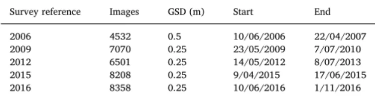
The regional orthophoto surveys in the study area are achieved by private operators on a regular basis, notably for the sake of controls related to European Union common agricultural policy. They were in-itially acquired on a triennial basis and since 2015, on an annual basis. The timetable of the regional surveys is driven by the objectives stated

above and typically ranges from April to October (Table 1). Such timetable can indeed lead to the acquisition of aerial images of decid-uous forest in leaf-off condition. Since the 2009 survey, the targeted Ground Sampling Distance (GSD) is 0.25 m in order to allow the pho-tointerpretation offine landscape features. The entire time series was acquired using Vexcel UltraCam Imaging Sensors ( https://www.vexcel-imaging.com/) based onflight plan using 60 % along-track and 30 % across-track overlaps. Such large frame sensors present low lens dis-tortion and provide a multispectral imagery covering the Red, Blue, Green and Near-Infrared spectral ranges.

We also used a regional LiDAR survey performed from 12 December 2012 to 09 March 2014. This LiDAR survey was used as a Digital Terrain Model (1 m GSD) to compute the pCHMs (photo. DSMs - ALS DTM) as well an ALS CHM (1 m GSD, ALS DSM - ALS DTM) to bench-mark the 5 pCHMs in terms of single tree height estimates.

2.3. Regional digital surface model 2.3.1. Photogrammetric reconstruction

We used Agisoft Metashape 1.5.4 in network mode for all the photogrammetric reconstruction steps synthetized inFig. 1. Agisoft is one of the most used photogrammetric packages using a multiview matching strategy (Smith et al., 2016). It also allows to handle large

images (200 Mpx and more) generated by large frame sensors like the UltraCam in an easy to set up network processing interface. We choose this software for its relatively user friendly GUI as well as its rather low cost (ca. 549 $ for educational license and 3500 $ for commercial li-cense) compared to other state-of-art photogrammetric package like Trimble Inpho or Imagine Photogrammetry (LPS). These characteristics will ease the reproducibility of the methodology.

We set up a processing network of 3–5 (depending on the resources available) computers equipped with GPU processing (NVidia GTX) and 64 Go RAM. The very same photogrammetric protocol was applied to process the raw images of the different regional orthophoto coverages. Based on the GNSS positions (metric coordinates system“Lambert 72”, EPSG: 31370) and the camera calibration information delivered by the service provider, we realized the tie point extraction in full resolution using the“High” accuracy parameter, “Key points limit” and “Tie point limit” set to 40,000 and 4000 respectively. To avoid overfitting, we followed the recommendations ofJames et al. (2017)and used a rather conservative lens calibration strategy. The following lens calibration parameters remained fixed: b1b2 (affinity and skew transformation coefficients), k4 and p3/p4 (additional tangential and radial distortion coefficients). This lens calibration strategy was pursuit during the entire photogrammetric processing. Thisfirst alignment process resulted in a first 3D reconstruction (sparse point cloud) based on an initial bundle block adjustment (BA) as highlighted inFig. 1-1.

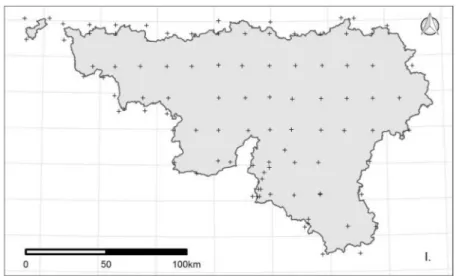
Based on this initial result, ground control points (GCP) were easily located on raw images thanks to the pre-positionning performed by the software. Two types of GCP were used to ensure and evaluate the quality of the photogrammetric reconstruction. A first set of GCP is based on a set of GCP network installed by the service provider who produced the orthophoto coverage for the 2012 survey. This network is made of 89 black and white circular marks (0.6 m radius) on the ground which can be easily located on the aerial images. All these points were accurately georeferenced on the ground using precision GNSS (Fig. 3-I). As this network was not available for the entire time series (2006 and 2009 surveys), we used a dense network (1088 units,Fig. 3-II) of re-ference ground marked points provided by the National Geographic Institute which consists of various particular points which can be seen on aerial images and have precisely been georeferenced on the ground with precision GNSS (pedestrian crossing, change in road color, …). The total GCP network represents an important reference dataset cov-ering the entire study area (Fig. 3-I and -II).

The accuracy assessment process is based on a cross-validation using repeated k-fold technique (k = 5, repetition = 50) implemented in Agisoft Metashape through python scripting. For each of the 50 itera-tions, the GCP dataset is randomly divided intofive folds of GCP and five BA processes are successively run (Fig. 2). Each BA process is run based on a set of GCP from one fold as checkpoint (not used in the process, i.e. test set), the other GCP (associated to the 4 other folds) being used as control points (to constrain the BA process, i.e. training set). The XYZ errors associated with the GCP from the test fold are saved and another BA is run, using GCP from one other fold as check-points. Once all the GCP’s from the k folds have been successively used as checkpoints (and thus as independent test set), the entire process is repeated over 50 times to ensure the robustness of the cross-validation. Indeed, all the GCP of the network are used to assess the 3D accuracy of the 3D reconstruction with 50 different neighboring conditions. As the accuracy of the 3D model is subsequently evaluated 50 times for each GCP, the XYZ error values were aggregated by mean. The quality of the photogrammetric DSMs wasfinally assessed through box-and-whisker plots as they allow to investigating the accuracy (i.e. mean/median error) and the precision (i.e. the deviation of error) as promoted in the guidelines proposed by James et al. (2019). The evenly spatial dis-tribution and the high density of the GCP network (1 GCP / 15 km²) allow avoiding the sampling of a test set of checkpoints within the GCP network and subsequently testing the entire network of ground control points. Once the accuracy assessment has been completed, all the GCP Table 1

Essential aerial survey parameters of regional orthophoto coverage.

Survey reference Images GSD (m) Start End

2006 4532 0.5 10/06/2006 22/04/2007

2009 7070 0.25 23/05/2009 7/07/2010

2012 6501 0.25 14/05/2012 8/07/2013

2015 8208 0.25 9/04/2015 17/06/2015

2016 8358 0.25 10/06/2016 1/11/2016

Fig. 1. Main steps of the photogrammetric workflow implemented in Agisoft Metashape. Data/Input are represented in solid white box, processes are in grey boxes and results are bolded, italicized and numbered from (1) to (4).

were used to run thefinal BA process (Figs. 1,2) with the GCP accuracy set to 0.01 m in the Agisoft interface.

The dense matching process was run using aggregated images (ag-gregation factor of 2, half resolution) as a compromise between spatial resolution and computing time. The “Aggressive” depth filtering strategy was selected to limit the noise in the dense cloud. Thefinal output is a DSM (“Interpolation” enabled) which results in 5 regional DSM in raster format (Figs. 1–4, 1 m GSD for the 2006 and 0.5 m for the other).

2.4. Regional photo Canopy Height Model (pCHM) 2.4.1. pCHM Processing

The regional photogrammetric DSMs were combined with a re-gional ALS Digital Terrain Model (photogrammetric DSM - ALS DTM) resampled according to the resolution of the DSMs. As the ALS survey occurred from 12 December 2012 to 09 March 2014 (see 2.2 section), we considered the topography as unchanged during the entire study period. As our study is dedicated to trees located inside forest land-scapes, this assumption is reasonable considering the low erosion rate in forested landscapes as well as the infrequency in the study area of catastrophic events (e.g. landslide or earthquakes).

2.4.2. Accuracy assessment of tree height estimates from pCHM

A selection offield reference plots from the regional FI program was performed using temporal and spatial criteria. The FI plots collect various parameters such as tree height, diameter at breast height (DBH), tree species, health condition, etc. The measurements of tree height were performed with a vertex ultrasound instrument. Measured trees are spatially located using azimuth and distance relative to the plot center which is georeferenced with off-the-shelf GNSS receivers. In terms of absolute positioning accuracy, a study conducted in a similar context in France (Monnet and Mermin, 2014) shows that such GNSS gives a plot positioning accuracy of 9 m ( ± 8.7 m). Thefield sampling is designed to cover the study area on a yearly basis. The ongoing in-ventory (second cycle) is a single-phase, non-stratified inventory using a systematic sampling design based on plots located at the intersections

of a 1,000 m (east-west) × 500 m (north-south) grid with 11,000 sampling plots located in the forest. Each year 10 % of all plots are assessed. They are selected on a systematic basis to be evenly dis-tributed throughout the region. Sampling plots is composed of con-centric circular plots with radius from 4.5 m to 18 m depending of the DBH class of the trees (Alderweireld et al., 2016). More information about the Walloon FI protocol can be found online (http://iprfw.spw. wallonie.be).

For every aerial survey, we selectedfield plots which were mea-sured in the same vegetative year (considering the growing cycle from April to October) in order to minimize errors linked to tree growth and tree removal. The relative position of the individual trees was converted to absolute ones based on the GNSS XY position of the plot center. As the plot centers are located using low-quality GNSS receivers, reloca-tion of thefield plot was mandatory and performed in QGIS 3.0 soft-ware (QGIS Delopment Team, 2020) by a trained operator. Using re-ference GIS layers (orthophoto based on photo. DSM and pCHM time series), the operator looked for the best XY shift and applied it to the entire trees of the FI plot. As the tree XY positions are relative to the stem position (at breast height) and not to tree tops, we used the method developed byEysn et al. (2015)to refine the individual trees location. This processing step also allows identifying trees from the upper canopy envelope as this information is not recorded during the field measurements of the FI. We performedFI trees XY position and height matching with local maxima detected in the associated pCHM by the tree_detection() function (lmf algorithm, adaptive moving windows based on tree height) of the lidR R package (Roussel and Auty, 2019). This results in a database of 1850 reference individual trees (Table 2) from 489 FI plots presenting an evenly spatial distribution in the study area. To avoid 3D reconstruction issues linked to (partial) leaf-off conditions, FI plots were selected only when they were in leaf-on condition during the associated aerial survey. In even-aged forests (mainly spruce and Douglasfir), the field survey of the tree height is limited to few individuals in order to compute the dominant height. As the evergreen forests are mainly managed as even-aged stands, they occur in a rather low proportion in the reference tree database as compared to deciduous trees. We performed the same matching be-tweenfield measured tree heights from FI plots and tree height esti-mates extracted from the ALS CHM. This database was composed of 1579 trees from 260 FI plots (1144 deciduous, 435 evergreen). The Fig. 3-III represents the FI plots network used in this study.

In order to test the reliability of tree height information provided by pCHM, we performed linear modelling between field measured tree height (from the reference tree database) and tree height estimates from local maxima of the 5 different pCHM’s. We applied a similar method with ALS reference dataset to benchmark tree estimates provided by the pCHM with a reference tree height remote sensing data source. 2.4.3. Drivers of the pCHM tree height estimates error

To investigate the robustness of the pCHM tree height estimates, we compared the impact of various parameters suspected to have an im-pact on the 3D reconstruction uncertainties or the tree height estimate itself (seeTable 3). Some parameters are assessed at the scale of the individual trees, others at the forest inventory plot scale. The mean solar angle of the aerial images is a good proxy for the light conditions during the surveys. Lower values can be associated to more important cast shadowing and higher reconstruction uncertainties. The time dif-ference between the aerial images could also highlight artificial het-erogeneity among aerial images which can hamper the photogram-metric 3D reconstruction. The number of overlapping images used for the photogrammetric reconstruction is in theory positively linked to the quality of the 3D reconstruction. As the 60 % along-tracks and 30 % across-track overlap scheme induces varying image overlap conditions, the number of images used to reconstruct the forest canopy of the FI plot is an interesting parameter. The uncertainties of the 3D photo-grammetric reconstruction of tree canopy can also be linked to the Fig. 2. K-fold process applied to assess the 3D accuracy associated with the GCP

set. GCP from the light grey folds are used as control points (training set), GCP from dark greyed fold are use as checkpoints (test set). This process was re-peated 50 times with error being aggregated by mean.

Fig. 3. Field reference data used in the different accuracy assessments of the study: I. black and white circular marks GCP (89), II. GCP from reference marked points provided by the National Geographic Institute (1088), III. forest inventory plots (610) used to complete an individual tree height reference database.

characteristic of the tree itself as well as its environment. The forest species and evergreenness were investigated as well as forest structure. Forest structure was here considered in terms of stem densities, canopy roughness and basal area within the FI plot. The relative DBH allows addressing the size of the considered tree in relation with the size of the biggest trees in the FI plot (i.e. proxy of the social status). Lastly, the terrain slope and altitude is also investigated as they can have a sig-nificant impact on the 3D reconstruction but also on the accuracy of the ALS DTM itself.

To evaluate the significance of the linear relationship between the selected parameters and the tree height absolute differences (abs(field tree height - pCHM tree height)), we used one-way analysis of variance, (ANOVA) for qualitative factors, and linear regressions for quantitative factors.

We ran a best subset regression approach to build a multivariate

linear model with the variables previously highlighted using the re-gsubsets tools from the leaps package in R (Miller, 2017). We used best subsets regression tofit all potential models of pCHM tree height esti-mate absolute error in order to highlight the best combination of pre-dictors (using bayesian information criterion, BIC)

Finally, we ran a second best subsets regression to test the potential of the highlighted parameters fromTable 3to improve the tree height estimates with pCHM’s data (using BIC).

3. Results

3.1. Accuracy assessment

The cross-validation process of the photogrammetric reconstruction highlights very low mean X, Y and Z error values associated with the 3D model of the aerial surveys (Fig. 4-I., II., III.). The XYZ error (Fig. 4-IV.) which is the root mean square of the X, Y and Z error is quite higher (ca. 0.7 m) but remains acceptable for all the surveys. It is worth mentioning that such low error values are associated to the 3D reconstruction of simple surfaces located in a homogeneous topography (mostly roads). The 3D reconstruction uncertainties are expected to be higher when the algorithms have to deal with complex surfaces like tree canopies.

The accuracy assessment of the tree height models highlights that the pCHM tree height estimates agreed well with thefield tree height estimates (Fig. 5). The r² values ranges from 0.84 to 0.88 with root mean square error (RMSE) values ranging from 1.91 to 2.08 m. A global modelfitted regardless the aerial survey (not plotted inFig. 5) on the pCHM and the FI tree height estimates reached similar performance with r² value of 0.87 and a RMSE of 2.01 m. The quality of the pCHM Fig. 4. Boxplot of the X, Y, Z and XYZ error resulting from the cross validation process. The XYZ error is the root mean square error of the 3 error components.

Table 2

Reference tree dataset used to assess the accuracy of tree height estimates based on Pchm.

Reference year (aerial survey) Reference tree

Total Evergreen Deciduous

2006 95 23 72 2009 380 63 317 2012 510 185 325 2015 246 152 94 2016 619 174 445 Total 1850 597 1253

tree height linear models is in line with the quality reached by the ALS CHM using the same approach (r² = 0.86; RMSE = 1.96 m). The Table 4gathers the results of the same modelling approach considering the deciduous and the evergreen species separately. Compared to de-ciduous species, the r² of the modelsfitted with evergreen species are higher (from 0.83 to 0.95) and the associated RMSE present lower values (from 1.4 to 1.7 m).

Our results also highlight a clear underestimation of the tree height by pCHM. The same trend is observed to a lesser extent for tree height based on ALS CHM. The mean tree height estimate error (FI tree height - pCHM tree height) ranges from 1.66 to 2.25 m for the pCHM estimates and 0.54 m for the ALS CHM. The mean tree height estimate error is higher for the evergreen species as it ranges from 2.5 to 3 m while it ranges from 0.92 to 2.02 m for deciduous species. The same trend can be observed in the ALS models but again with lower mean error values (< 1 m).

3.2. Drivers of the pCHM tree height estimates error

Among the 13 potential parameters listed inTable 3, our analysis highlighted 8 variables which present a significant statistical link with the absolute error of the pCHM height estimates (Table 5). Except the basal area and the number of trees in the FI plots, all the forest para-meters were selected as well as the topographic parapara-meters (slope and altitude). In terms of correlation, the slope is the only parameter which presents a negative correlation coefficient with the pCHM absolute error.

The reference year of the aerial survey is the only image parameter which was highlighted by our analysis. As the number of levels in the factor is rather low for this variable, we ran a Tukey Honest Significant Differences implemented in the TukeyHSD function in the R basic package. This test highlighted that only the observations from the aerial surveys 2015 and 2016 were significantly different (p-value = 0.011). Within the set of variables which were proved to have a significant statistical relationship with the pCHM tree height absolute error, we removed the reference year and the tree species factorial variables before running the best subset regression process. This choice was made in order to ease the interpretation (the Speciestreefactor presents 29

le-vels in our dataset) and the replication of thefitted pCHM error model. Indeed, the aerial survey reference gathers a bunch of environmental parameters at the time of theflight survey (lights conditions, phenology …) with a rather low interest for understanding the drivers of the pCHM tree height estimates error.

The best subsets regression model selected following the BIC a

model with 2 variables: the DBH and the evergreenness factor to predict pCHM tree height estimate error. This model presents a rather low r² score (0.10) and a RMSE of 1.3 m.

Finally, we used the same initial set of variables used tofit the pCHM tree height estimate error model to evaluate their potential in-come in terms of accuracy improvement of a global model linking the tree height estimates provided with pCHM data (all pCHM used) and the FI tree height estimates. The best subsets regression model selected (using BIC) a model with 4 variables to predict thefield measured tree height: the pCHM tree height, the DBH, the evergreenness factor and the terrain slope. This model is significantly different (ANOVA test, p-value < 0.001) of the linear model linking pCHM tree height andfield measured tree height. It presents a slightly higher r² score (0.90 VS 0.87) and a smaller RMSE (1.78 VS 2.01 m). Therefore, the use of these variables in a multiple linear model improved the tree height estimate based on pCHM.

4. Discussion

4.1. Accuracy of tree height estimates with pCHM

The good agreement between the pCHM andfield tree height esti-mates was clearly highlighted by thefitted linear models. They reached similar performance than ALS tree height estimates model. Globally, pCHM and ALS CHM underestimate thefield measured tree height es-timate (seeTable 4). This was commonly found in literature by various authors likeHeurich et al. (2004). Nevertheless, the ALS tree height estimate remains more accurate with mean signed error (field height -CHM height) being submetric (0.54 m for evergreen and deciduous species) while pCHM mean signed error being more than three times higher (1.85 m for all pCHM, evergreen and deciduous species).

While the mean difference between pCHM and field tree height estimates is more important for evergreen species than for deciduous ones, the performance of the modelfitted with evergreen tree species is better with r² values above 0.9 and model RMSE below 2 m. On one hand, the larger difference between pCHM and field tree height esti-mates for evergreen species can be associated to their higher mean height in the study area. On the other hand, the better model perfor-mance is also probably related to their simpler canopy structure. These results are in line with a lot of studies having compared the single tree height modeling with CHM (pCHM or ALS CHM) asGinzler and Hobi (2015)for a pCHM case study.

It is worth noting that the 2006 survey presents similar results but with slightly lower model performance and higher mean error values. Table 3

Parameters and associated explanatory variables used to assess the robustness of tree height from pCHM. The relative diameter is the ratio of the DBH of tree (DBHtree) and the mean DBH of the 100 biggest trees / acre (dominant DBH, DBHdominant) for the FI plot.

Parameter Symbol Explanatory variable Rationale Scale Type of parameter

Sun angle during aerial image survey

Sunangle Mean sun azimuth of aerial images

overlapping (angular degree)

Low solar angle induces cast shadow FI plot Image survey

Overlapping images OverlapIm. Number of images overlapping Higher overlaps improves 3D reconstruction quality FI plot Image survey

Time difference Timedif Max time difference between the survey of

the aerial images (day)

Noise induced by varying phenological states FI plot Image survey

Aerial survey Refaerial Reference year of the associated pCHM Test differences among aerial surveys FI plot Image survey

Basal area Basalarea Basal area (m²/Ha) Forest structure is linked to 3D reconstruction

uncertainty

FI plot Forest

Stem density Stemdens Number of stem by hectare FI plot Forest

Canopy roughness Canopyrough. Variation Coefficient of associated pCHM

(%)

FI plot Forest

Stem diameter at breast height

DBH DBH (cm) Impact of tree size or species characteristics Tree Forest

Relative diameter DBHrel DBHtree

DBHdominant

Trees (understory or with lower leaf amount) are unlikely to be reconstructed in pCHM

Tree / FI plot

Forest

Tree species Speciestree Tree species Tree Forest

Evergreenness Evergreen Deciduousness/Evergreenness Tree Forest

Altitude Altitude Mean ALS DTM altitude Impact of ecological/geographical context FI plot Topo.

These results are probably directly linked to the lower spatial resolution of the pCHM (1 m GSD) even if our study design does not permit to further proof it.

Our results are in line with those obtained with pCHM approaches at a smaller study area extents byZimmermann and Hoffmann (2017)or Hirschmugl et al. (2007)even if the lack of harmonized accuracy me-trics hampers real accuracy benchmarking. The most similar case

studies found in literature is fromGinzler and Hobi (2015)whofitted with pCHM a tree height estimate model based on 3109field measured trees with r² of 0.68. Our slightly better results in terms of accuracy/ performance can be linked to the geographical context (mountainous complex landscapes VS lowlands / low mountain landscapes) and the tree top position extraction algorithm (fixed buffer around ground GNSS position VS matched position with local maxima) or even the Fig. 5. Biplots of tree height estimates from pCHM’s and ALS CHM in comparison with FI tree height estimates. Deciduous and evergreen trees are marked using “+ “and “.” symbols respectively. The mean error (err.) is computed from the difference between the reference tree height (from FI) and the tree height estimates (provided by pCHM or ALS CHM).

image matching strategy (stereo matching VS multiview matching). 4.2. Drivers of the pCHM tree height estimates error

Our results in Table 5 highlight the significant impact of all the forest parameters except the basal area and the number of trees in the FI plots. This draws attention on a subject poorly addressed in literature: the relationship between forest structure and DAP products quality at the single tree scale. If the impact of leaf abundance is well addressed in literature (seeHuang et al. (2019)for a recent case study), our results in Table 5draw attention on parameters which should be addressed by researchers: the canopy roughness, the tree size (both absolute and relative to its neighbors), the tree species, the deciduousness/ever-greenness as well as the topography (slope and altitude). In our results, all of the parameters except the slope are positively correlated with the absolute pCHM tree height estimate error. These results could be syn-thetized as the bigger the tree is, the bigger the error of its pCHM height estimate is. The positive correlation between the canopy roughness (assessed here through the pCHM coefficient of variation in the FI plot) can be interpreted by the lower ability of DAP to model high slope variation, especially when considering the rather low overlap of our aerial images dataset (60 % along-track, 30 % across-track) as sug-gested byHirschmugl et al. (2007). The altitude is generally considered as a very good proxy of the ecological gradient in various studies in the study area (Brogna et al., 2018;Dufrene and Legendre, 1991;Georges et al., 2019). Beside the link with an ecological gradient, the positive correlation with the absolute pCHM height estimate error can partially be linked to the tendency of evergreen stands to be located in higher altitude while having a higher height. The negative correlation between

the absolute pCHM height estimate error and the terrain slope is quite counterintuitive as CHMs tend to overestimate the actual tree height in steep slope areas (Khosravipour et al., 2015). This overestimation could thus partially counter the general trend to underestimation by pCHM previously highlighted. Subsequently, the surprisingly negative corre-lation is interpreted as a compensation effect.

Among the variables related to the image acquisition, only the re-ference of the aerial survey was highlighted by our analysis. The ab-sence of impact of the sun light condition during the survey can be related to the rather strict conditions asked to the service provider. Our analysis focused on tree tops from the upper canopy layer, the sun light condition (and associated cast shadows) as well as the images overlap are expected to be of higher importance for studies dealing with canopy gaps for example (Hirschmugl et al., 2007) or when working on lower canopy attributes.

Among the parameters underlined in thisfirst analysis, the best subsets regression highlighted the DBH and the evergreenness factor as the best predictors of the absolute pCHM tree height estimate error. This result highlights some interesting potential drivers of the pCHM tree height estimate error but it also highlights that a significant part of its variability was not addressed with these set of parameters. Nevertheless, the use of the same initial set of variables used tofit a model predicting thefield measured tree height produced interesting results. The use of these additional variables allows to significantly improving the tree heightfield measurement model (ANOVA test, p-value < 0.001) in terms of r² and RMSE.

In our study, we considered thefield measured tree height as the reference information for the benchmarking of the tree height estimate with the pCHM. Nevertheless, tree height estimates from the ground are both subject to instrumental and measurement errors. As the field height data were collected using ultrasound equipment which tends to have low instrumental errors (if properly maintained), the most im-portant potential errors are suspected to occur in the measurement step itself.Rondeux (1999)highlighted that tree height measurement errors can be considered as random. They are linked to the shape of the tree and its position, the equipment set-up or even thefield operator him-self. More recently, Wang et al. (2019) highlighted that field mea-surements tend to overestimate the height of tall trees but also that this trend was more related to non-dominant individuals trees (co-domi-nant, intermediate, suppressed). Our study design did not allow the evaluation of thefield measurement error among pCHM tree height estimate error. Nevertheless, the values of the slope parameter in the different fitted models was close to 1 for the linear models inFig. 5. This result highlights that the differences between field and pCHM tree height measurements tend to remain relatively constant across the tree height range in our datasets.

5. Conclusions

Our results allow highlighting the good agreement of tree height estimates provided by pCHM using DAP with bothfield measured and ALS tree height data. In terms of tree height modeling, our pCHM ap-proach reached similar results than the same modeling strategy applied to ALS tree height estimates. Our results highlight the interest of re-processing stereo-images acquired during regular national campaigns for orthophotomosaics layers production in order to produce regional pCHM. We tested it at a regional scale (ca. 17,000 km²) using 5 dif-ferent aerial surveys and a large single tree and FI plots dataset (ca. 3000 trees from 600 FI plots). Our approach presents a great potential as it relies on publically and regularly acquired datasets (aerial images and FI data) and could be thus easily replicated in other countries to build dense time series of pCHM. These time series can cover time periods prior the ALS survey when the hypothesis of constancy of to-pography under forest cover can be realized.

Our study also identified some of the drivers of the pCHM tree height estimate error and found forest parameters and the terrain slope Table 4

Tree height estimates with pCHM and ALS CHM compared to tree estimates from FI.

Aerial survey Evergreen Deciduous

r² RMSE (residuals) Mean error (y-x, m) r² RMSE (residuals) Mean error (y-x, m) 2006 0.83 1.68 3 0.83 2.17 2.02 2009 0.92 1.67 2.92 0.87 1.92 1.68 2012 0.91 1.72 2.52 0.83 2.03 1.4 ALS CHM 0.92 1.6 0.6 0.82 2.07 0.52 2015 0.93 1.43 3.05 0.88 1.92 0.92 2016 0.95 1.51 2.76 0.86 2.08 1.23 All photo surveys 0.93 1.59 2.78 0.87 2.01 1.85 Table 5

Parameters and associated explanatory variables used to assess the robustness of tree height from pCHM. For linear model, AH0 (acceptation of null hy-pothesis) stands for no relationship among the variables and for ANOVA models, AH0 implies equality of means between the groups.

Symbol Model Results DAP

Sunangle Linear regression AH0 (p = 0.65)

Overlap_Im. Linear regression AH0 (p = 0.12)

Timedif Linear regression AH0 (p = 0.38)

Ref_aerial ANOVA RH0 (p = 0.004)

Basalarea Linear regression AH0 (p = 0.11)

Stemdens Linear regression AH0 (p = 0.55)

Canopyrough. Linear regression RH0 (p = 0.020; r = 0.05)

DBHtrunk Linear regression RH0 (p < 0.001; r = 0.09)

DBHrel Linear regression RH0 (p < 0.001 ; 0.13)

Speciestree ANOVA RH0 (p < 0.001)

Evergreen ANOVA RH0 (p < 0.001)

Altitude Linear regression RH0 (p < 0.001; r = 0.11)

to be of higher importance than image survey parameters like the variation of the overlap or the sunlight condition in our dataset. In combination with the pCHM tree height estimate; the terrain slope, the DBH and the evergreenness factor were used tofit a multivariate model predicting thefield measured tree height. This model presented better performance than the model linking the pCHM estimates to thefield tree height estimates in terms of r² (0.90 VS 0.87) and RMSE (1.78 VS 2.01 m). As the integration of these environmental parameters is rather straightforward, these results could be further used to improve plot scale forest attributes prediction based on DAP and pCHM. Such aspects are poorly addressed in literature and further research should focus on how pCHM approaches could integrate them to improve forest char-acterization using DAP and pCHM.

Our promising results can be used to encourage the use of regional aerial orthophoto surveys archive to produce large scale quality tree height data at very low additional costs, notably in the context of up-dating national forest inventory programs.

CRediT authorship contribution statement

Adrien Michez: Conceptualization, Methodology, Investigation, Formal analysis, Writing - original draft, Writing - review & editing.Leo Huylenbroeck: Conceptualization, Methodology, Writing - original draft, Writing - review & editing.Corentin Bolyn: Conceptualization, Methodology, Writing - original draft, Writing - review & editing. Nicolas Latte: Conceptualization, Methodology, Writing - original draft, Writing - review & editing. Sébastien Bauwens: Conceptualization, Methodology, Writing - original draft, Writing - re-view & editing. Philippe Lejeune: Conceptualization, Methodology, Writing - original draft, Writing - review & editing.

Declaration of Competing Interest

The authors declare that they have no known competingfinancial interests or personal relationships that could have appeared to in flu-ence the work reported in this paper.

Acknowledgments

Authors thank the Belgian National Geographic institute for having shared their reference point database. Authors would also like to thank Alain Monseur, Coralie Mengal and Thibault Delinte for their technical support.

Authors express thanks to the Public Service of Wallonia has shared all the dataset and associated expertise from the aerial images (Geomatic Directorate: C. Schenke, N. Stephenne and JC Jasselette) to the forest information from the Forest Inventory program (Forest Resources Department).

Finally, authors would like to thanks the funding agencies who provided support to our research: the Stereo program (grants SR/00/ 347 and SR/12/383) from the Belgian Scientific Policy Department (BELSPO) and the Forest Resources Department of the public service of Wallonia (accord cadre de recherche et de vulgarization forestière 2014-2019).

References

Alderweireld, M., Burnay, F., Pitchugin, M., Lecomte, H., 2015. Inventaire Forestier Wallon-Résultats 1994-2012. SPW.

Alderweireld, M., Rondeux, J., Latte, N., Hébert, J., Lecomte, H., 2016. National Forest Inventories. Springer, Belgium (Wallonia), pp. 159–179.

Brogna, D., Dufrêne, M., Michez, A., Latli, A., Jacobs, S., Vincke, C., Dendoncker, N., 2018. Forest cover correlates with good biological water quality. Insights from a regional study (Wallonia, Belgium). J. Environ. Manage. 211, 9–21.

Dufrene, M., Legendre, P., 1991. Geographic structure and potential ecological factors in Belgium. J. Biogeogr. 257–266.

Eysn, L., Hollaus, M., Lindberg, E., Berger, F., Monnet, J.-M., Dalponte, M., Kobal, M., Pellegrini, M., Lingua, E., Mongus, D., et al., 2015. A benchmark of lidar-based single tree detection methods using heterogeneous forest data from the alpine space. Forests 6, 1721–1747.

Georges, B., Brostaux, Y., Claessens, H., Degré, A., Huylenbroeck, L., Lejeune, P., Piégay, H., Michez, A., 2019. Can water level stations be used for thermal assessment in aquatic ecosystem? River Res. Appl.

Ginzler, C., Hobi, M., 2015. Countrywide stereo-image matching for updating digital surface models in the framework of the Swiss National Forest Inventory. Remote Sens. 7, 4343–4370.

Goodbody, T.R., Coops, N.C., White, J.C., 2019. Digital aerial photogrammetry for up-dating area-based forest inventories: a review of opportunities, challenges, and future directions. Curr. For. Rep. 5, 55–75.

Heurich, M., Persson, A.A., Holmgren, J., Kennel, E., 2004. Detecting and measuring individual trees with laser scanning in mixed mountain forest of central Europe using an algorithm developed for Swedish boreal forest conditions. Int. Arch. Photogramm. Remote Sens. Spat. Inf. Sci. 36, W2.

Hirschmugl, M., Ofner, M., Raggam, J., Schardt, M., 2007. Single tree detection in very high resolution remote sensing data. Remote Sens. Environ. 110, 533–544. Huang, H., He, S., Chen, C., 2019. Leaf abundance affects tree height estimation derived

from UAV images. Forests 10.https://doi.org/10.3390/f10100931.

James, M.R., Robson, S., d’Oleire-Oltmanns, S., Niethammer, U., 2017. Optimising UAV topographic surveys processed with structure-from-motion: Ground control quality, quantity and bundle adjustment. Geomorphology 280, 51–66.

James, M.R., Chandler, J.H., Eltner, A., Fraser, C., Miller, P.E., Mills, J.P., Noble, T., Robson, S., Lane, S.N., 2019. Guidelines on the use of structure-from-motion pho-togrammetry in geomorphic research. Earth Surf. Process. Landf.

Keenan, R.J., Reams, G.A., Achard, F., de Freitas, J.V., Grainger, A., Lindquist, E., 2015. Dynamics of global forest area: results from the FAO global forest resources assess-ment 2015. For. Ecol. Manag. 352, 9–20.

Khosravipour, A., Skidmore, A.K., Wang, T., Isenburg, M., Khoshelham, K., 2015. Effect of slope on treetop detection using a LiDAR Canopy Height Model. ISPRS J. Photogramm. Remote Sens. 104, 44–52.

Leberl, F., Irschara, A., Pock, T., Meixner, P., Gruber, M., Scholz, S., Wiechert, A., 2010. Point clouds. Photogramm. Eng. Remote Sens. 76, 1123–1134.

McRoberts, R.E., Tomppo, E.O., 2007. Remote sensing support for national forest in-ventories. Remote Sens. Environ. 110, 412–419.

Michez, A., Bauwens, S., Bonnet, S., Lejeune, P., 2016. Characterization of forests with lidar technology. Land Surface Remote Sensing in Agriculture and Forest. Elsevier, pp. 331–362.

Miller, T.L., 2017. leaps: Regression Subset Selection. based on F. code by A...

Monnet, J.-M., Mermin, É., 2014. Cross-correlation of diameter measures for the co-re-gistration of forest inventory plots with airborne laser scanning data. Forests 5, 2307–2326.

Næsset, E., 2014. Area-based inventory in Norway–from innovation to an operational reality. Forestry Applications of Airborne Laser Scanning. Springer, pp. 215–240.

QGIS Delopment Team, 2020. QGIS Geographic Information System. Open Source Geospatial Found. Proj.QGIS Geographic Information System. Open Source Geospatial Found. Proj.

Rahlf, J., Breidenbach, J., Solberg, S., Næsset, E., Astrup, R., 2017. Digital aerial photo-grammetry can efficiently support large-area forest inventories in Norway. For. Int. J. For. Res. 90, 710–718.

Rondeux, J., 1999. La Mesure Des Arbres Et Des Peuplements Forestiers. Les presses agronomiques de Gembloux.

Roussel, J.-R., Auty, D., 2019. lidR: Airborne LiDAR Data Manipulation and Visualization for Forestry Applications.

Smith, M., Carrivick, J., Quincey, D., 2016. Structure from motion photogrammetry in physical geography. Prog. Phys. Geogr. 40, 247–275.

Wang, Y., Lehtomäki, M., Liang, X., Pyörälä, J., Kukko, A., Jaakkola, A., Liu, J., Feng, Z., Chen, R., Hyyppä, J., 2019. Isfield-measured tree height as reliable as believed–A comparison study of tree height estimates fromfield measurement, airborne laser scanning and terrestrial laser scanning in a boreal forest. ISPRS J. Photogramm. Remote Sens. 147, 132–145.

White, J.C., Wulder, M.A., Vastaranta, M., Coops, N.C., Pitt, D., Woods, M., 2013. The utility of image-based point clouds for forest inventory: a comparison with airborne laser scanning. Forests 4, 518–536.https://doi.org/10.3390/f4030518.

Zimmermann, S., Hoffmann, K., 2017. Accuracy assessment of normalized digital surface models from aerial images regarding tree height determination in Saxony, Germany. PFG–J. Photogramm. Remote Sens. Geoinf. Sci. 85, 257–263.