Inférence pour des processus affines basée sur des observations à temps discret

INFÉRENCE POUR DES PROCESSUS AFFINES

BASÉE SUR DES OBSERVATIONS

À

TEMPS DISCRET

MÉMOIRE

PRÉSENTÉ

COMME EXIGENCE PARTIELLE

DE LA MAîTRISE EN MATHÉMATIQUES

PAR

MARYAMLOLO

Service des bibliothèques

Averiissement

La diffusion de ce mémoire se fait dans le respect des droits de son auteur, qui a signé le formulaire Autorisation de reproduire et de diffuser un travail de recherche

de cycles supérieurs (SDU-522 - Rév.01-2006). Cette autorisation stipule que

«conformément

à

l'article 11 du Règlement nOS des études de cycles supérieurs, [l'auteur] concède

à

l'Université du Québec

à

Montréal une licence non exclusive d'utilisation et de publication de la totalité ou d'une partie importante de [son] travail de recherche pour des fins pédagogiques et non commerciales. Plus précisément, [l'auteur] autorise l'Université du Québec

à

Montréal

à

reproduire, diffuser, prêter, distribuer ou vendre des copies de [son] travail de recherche

à

des fins non commerciales sur quelque support que ce soit, y compris l'Internet. Cette licence et cette autorisation n'entrainent pas une renonciation de [la] part [de l'auteur]

à

[ses] droits moraux ni

à

[ses] droits de propriété intellectuelle. Sauf entente contraire, [l'auteur] conserve la liberté de diffuser et de commercialiser ou non ce travail dont [il] possède un exemplaire.»

1 am heartily thankful to my supervisor, René Ferland, whose encouragement, guid­ ance and support enabled me to develop an understanding of the subject.

Myparents, Parvin and Ahmad, and my sister, Shaghayegh have been a constant source of support, and this thesis would certainly not existed without their supports and 1 thank ,them, Lastly, 1 offer my regards and blessings to ail of those who supported me in any re­

LIST OF TABLES .. v LIST OF FIGURES. vi RÉSUMÉ . . . x ABSTRACT .. xi INTRODUCTION CHAPTER 1

STOCHASTIC DIFFERENTlAL EQUATIONS 3

1.1 ODE as a modeling tool . 3

1.2 Brownian motion and Wiener integrals 4

1.3 Linear stochastic differential equation 6

1.4 Nonlinear stochastic differential equations . 9

1.5 Systems ofSDEs . 10

1.6 Affine models and zero-coupon formulas. 11

1.6.1 Single-factor models 12

1.6.2 Multi-factor models 13

CHAPTER II

MAXIMUM LIKELIHOOD ESTIMATION 15

2.1 General principles .. . . . . 15

2.2 MLE for the Vasicek process . 17

2.3 MLE for the square root process 21

2.4 Numerical examples 23 CHAPTER III ZERO-COUPON DATA 34 3.1 Zero-coupon priees. 34 3.2 Single-factor models 36 3.3 Multi-factor models 37

3.4 Maximum likelihood estimation 39

3.5 Numerical analysis 40

CHAPTER N

KALMAN FILTERING 50

4.1 Introduction ta Kalman Altering 50

4.2 The state-space formulation .. 54

4.2.1 Vasicek model . 54

4.2.2 The

cm

model 57

4.3 The Kalman Alter implementation .. 59

4.4 Maximum likelihood estimation 61

4.5 Numerical analysis .. 62

CONCLUSION. 71

APPENDIX A

SIMULATION RESULTS FOR MAXIMUM LIKELIHOOD METHOD 72

APPENDIX B

SIMULATION RESULTS FOR INDIRECT MAXIMUM LIKELIHOOD METHOD . . . . .. S4 APPENDIX C

SIMULATION RESULTS USING KALMAN FILTERING .. . . .. 96 APPENDIX D

MATLAB CODE FOR SIMULATION AND ESTIMATION IDS

D.l Code for Chapter II .. IDS

D.l.l Vasicek Madel . lOS

D.1.2

cm

Madel . . . III

D.2 Code for Chapter III . 113

D.2.1 Vasicek Madel . . . 113

D.2.2

cm

Madel . . . 115

D.3 Code for Chapter N . 117

D.3.1 Vasicek Madel .. 117

D.3.2

cm

Madel . 120

2.1 A simulation analysis of the MLEs with n = 100 observations . . . .. 31 2.2 A simulation analysis of the MLEs with n =500 observations 32 2.3 A simulation analysis of the MLEs with n = 1000 observations. 33

3.1 A simulation analysis of the MLEs for zero-coupon data witl.1 n = 100 observa­ tions. . . . .. 47 3.2 A simulation analysis of the MLEs for zero-coupon data with n = 500 observa­

tions , 48

3.3 A simulation analysis of the MLEs for zero-coupon data with n = 1000 obser­ vations . . . .. 49

4.1 A simulation analysis using Kalman filter for n = 100 observations . . . .. 68 4.2 A simulation analysis using Kalman filter for n = 500 observations 69 4.3 A simulation analysis using Kalman filter for n = 1000 observations . . . .. 70

2.1 Generated samp!e paths for the Vasicek process , , . . . . . , , , , , , . , " 25 2.2 Generated samp!e paths for Cox-Ingersoll-Ross process . . . . .. 26 2.3 Empirical distribution of K for the Vasicek mode! with parameters

<Pl . . . . ..

27 2.4 Empirical distribution of K for the

cm

mode! with parameters

<Pl

,

28 2.5 Empirical distribution of

ê

for the

cm

model with parameters <P2 ,. 29 2.6 Empirical distribution of Ô' for the

cm

mode! with parameters <P2 ' . . . " 30

3.1 Generated priees for the Vasicek mode! . 41

3.2 Generated prices for the Cox-Ingersoll-Ross mode! , . . . .. 42 3.3 Empirical distribution of K with zero-coupon data for the Vasicek mode! with

parameters <P2 . . . . . . . . , . . . , . , , .. 43 3.4 Empirical distribution of Ô' with zero-coupon data for the Vasicek mode! with

parameters <P2 . . . . , , . . . , , . . . , . .. 44

3.5 Empirical distribution of K with zero-coupon data for the

cm

mode! with pa­

rameters <P2 , .. , , , , . . . 45

3,6 Empirica! distribution of

ê

with zero-coupon data for the

cm

mode! with pa­

rameters

<Pl

" . . . . ..

46

4,1 Empirical distribution of Ô' for zero-co~pon data and Ka!man fi!tering (Vasicek

• •

4.2 Empirical distribution of Ct for zero-coupon data and Kalman filtering (Vasicek

mode! with parameter r.!J2). . • • . . . • . • . . . • . . . • . . . 65 4.3 Empirica! distribution of

ê

for zero-coupon data and Kalman fi!tering (CIR

mode! with parameter

r.!JIl. .

: . . .

66 4.4 Empirica! distribution of f( for zero-coupon data and Kalman filtering (CIR

mode! with parameter 4>2). . : . . . 67

A.l Empirical distribution ofMLE Kfor Vasicek's mode!.

· ....

·

..

• 1 72

A2 Empirical distribution of MLE Kfor Vasicek's mode!.

_{· .}

_{· .}

_·

_.

_{· .}

73

A.3 Empirical distribution ofMLE

ê

forVasicek's mode!. .. · .. · . . . 74

A.4 Empirica! distribution of MLE

ê

for Vasicek's mode!.

· ....

·

..

_{· . · .}

75

A.5 Empirical distribution of MLE {j for Vasicek's modeI.

· .. · ..

.

.... 76

A.6 Empirical distribution ofMLE {j forVasicek's mode!.

_{· .}

·

_.

·

...

· . · .

77

A.7 Empirical distribution ofMLE Kfor the CIR mode!.

.. ·

..

·

...

·

.

·

.

78

A.8 Empirical distribution ofMLE Kfor the CIR modeI.

_{· .}

_·

_{. · .}

79 A9 Empirical distribution of MLE

ê

forthe CIR mode!.

· .

· .

80

AIO Empirical distribution ofMLE

ê

for the CIR mode!. 81

AlI Empirica! distribution of MLE {j for the CIR mode!. . . .. 82

A.12 Empirical distribution ofMLE {j for the CIR mode!. . . .. 83

B.l Empirica! distribution of MLE K for Vasicek's mode! (zero-coupon data). 84

B.2 Empirical distribution of MLE K for Vasicek's mode! (zero-coupon data). 85

BA Empirical distribution of MLE

ê

for Vasicek's model (zero-coupon data), 87 B.S Empirical distribution of MLE {j for Vasicek's model (zero-coupon data). 88 B.6 Empirical distribution of MLE {j for Vasicek's model (zero-coupon data). 89 B.7 Empirical distribution ofMLE Kfor the

cm

model (zero-coupon data). 90 B.8 Empirical distribution ofMLE Kfor the

cm

model (zero-coupon data). 91 B.9 Empirical distribution ofMLE

ê

forthe

cm

model (zero-coupon data). 92 B.IO Empirical distribution ofMLE

ê

for the

cm

model (zero-coupon data). 93

B.n

Empirical distribution ofMLE {j for the

cm

model (zero-coupon data). . 94

B.12 Empirical distribution ofMLE {j for the

cm

model (zero-coupon data). . 95

C.l Empirical distri bu tion of Quasi -MLE K for Vasicek's mode!.

_{· .}

· ...

96 C.2 Empirical distribution of Quasi-MLE K for Vasicek's mode!.

·

....

· ..

97

C.3 Empirical distribution of Quasi-MLE

ê

for Vasicek's mode!.

...

· .

98

CA

Empirical distribution ofQuasi-MLE

ê

forVasicek's mode!.

...

· .

99

c's

Empirical distribution of Quasi- MLE {j for Vasicek's mode!.

· ..

.

. ·

.

100

C.6 Empirical distribution of Quasi-MLE {j forVasicek's mode!.

·

....

·

.

101 C.7 Empirical distribution of Quasi-MLE K for the

cm

mode!.

...

· ...

· .

102 C.8 Empirical distribution of Quasi-MLE K for the

cm

mode!.

....

· ..

103

C.9 Empirical distribution of Quasi-MLE

ê

for the

cm

mode!. ·

.. .

.

104 C.lO Empirical distribution of Quasi-MLE

ê

for the

cm

mode!.

..

_{· .}

_{· . ·}

_.

105 C.ll Empirical distribution of Quasi- MLE {j for the

cm

mode!. . 106

Dans ce mémoire, on étudie la distribution empirique des estimateurs de vraisem­ blance maximale pour des processus affines, basés sur des observations à temps discret. On examine d'abord le cas où le processus est directement observable. Ensuite, on regarde ce qu'il advient lorsque seule une transformation affine du processus est observable, une situa­ tion typique dans les applications financières. Deux approches sont alors considérées: maxi­ misation de la vraisemblance exacte ou maximisation d'une quasi-vraisemblance obtenue du filtre de Kalman.

Mots-clés: estimation devraisemblance maximale, processus affines, obligation à l'escompte, quasi-vraisemblance, filtre de Kalman.

In this dissertation, we study the empirical dis tribu tion of the maximum likelihood es­ timator for affine pro cesses, based on discrete sam pie data. We first study the case where the pro cess is directly observable. Then we look at what happens if only an affine transforma­ tion of the data is observable. a typical situation in financial applications. Two approaches are considered: maximisation of the exact Iikelihood or maximisation of a quasi-Iikelihood computed via Kalman filteril)g.

Keywords: maximum Iikelihood estimation, affine processes, zero-coupon bond, quasi-Iike­ Iihood, Kalman's filter.

This dissertation is concerned with the parameter estimation of affine processes used to describe the term structure of interest rates. Many methods have been proposed for this purpose, most of them being essentially variations of maximum likelihood estimation. Our presentation is divided into two parts. The first part provides an overview of concepts re­ quired to understand the term structure literature used in finance, whieh uses stochastic differential equations (SDEs) to show the dynamies of a zero-coupon bond. This develop­ ment begins with a single-factor model and then generalizes to higher dimensions. Further, we study the relation between state variables and bond priees. Since the term structure of interest rates is never observed in continuous time, we consider an estimation method based on discrete-time data. The second part discusses and compares different approaches to find an accurate method that can beused to estimate the unknown parameter set at each of these term-structure models. We conduct an empirieal study for each of these methods.

The first chapter includes an introduction to the theory and implementation of the class of affine term structure models. A variety of models exist, including those suggested by Duffie and Kan (1996), Vasieek (1977), Cox, Ingersoll and Ross (l985a), Longstaff and Schwartz (1992a) and Chen (1995). This dissertation focuses on the theoretical formulation of the Vasicek and

cm

single and multi-factor affine models.

In the second chapter we present maximum likelihood estimation for stochastic dif­ ferential equations based on a direct observation of the process itself. For the SDEs consid­ ered here, this is rather straightforward. For nonlinear SDEs the problem is more difficult and will not be addressed here. However, for a more detaiIed discussion of these issues, one can look at Pederson (1995), Cox, Ingersoll and Ross (1985b), Lo (1988) and Gourieroux and Jasiak (2001).

In the third chapter we consider maximum likelihood estimation for the term struc­ ture models introduced in Chapter l, and we study the empirical performance of the sug­ gested estimator on two examples. The study begins with the single factor models and then generalizes these concepts into a multi-dimensional setting. Empirical papers that explore this issue in detail include Cox, lngersoll and Ross (1985b), Geyer and Pichler (1999) and Bolder (2001).

The final chapter summarizes the material on the state-space models and introduces another technique to estimate unknown parameters, a technique called Kalman filtering. We then apply Kalman filtering to the simulated data of the previous chapter and compare the results.

STOCHASTIC DIFFERENTIAL EQUATIONS

1.1 ODE

as

a modeling tool

Differential equations consist of an unknown function of one or several variables whieh re­ lates to the values of the function itself and of its derivatives of various order. Many laws in Physies, Chemistry, Engineering and Economies can be expressed in the simplest way by differential equations. For example, let X( t) represent one coordinate of the position of a particle in space; then X' (t) and X" (t) represent the velocity and the acceleration of the par­ ticle at time t. Let m denote the mass of the particle and let F(t) denote the force acting on the particle at time t. By Newton's law,

F(t) = mX"(t). (1.1.1)

Usually, F(t) consist of three types of forces:

a) a frietional force -

f

X' (t), b) a restoring force -kX(t),

c) an external force ç(t), whieh is independent of the motion.

Therefore, we may write F( t) with respect to these types of forces as

By combining (1.1.1) and (1.1.2) we obtain the differential'equation

mX"(t)

+

f

X' (t)

+

kX(t)

=

ç(t).

Ifthe differential equation con tains functions of only one independent variable, and one or more of its derivatives with respect to that variable, we caB it an ordinary differential equa­ tion (ODE); thus, the above example is an ODE.

ODEs frequently appear in the natunil and physical models but in reality some pa­ rameters may not be deterministic and we should consider them as random variables. For example, if we suppose that the external force is due to sorne random effect, then in the abcive case we can think of ç(t) as a collection ofrandom variables which change by time t.

1.2 Brownian motion and Wiener integrals

So far, we found that for modeling a natural event we can use an ordinary differential equation which has a random process component. Now the question is, how can we model this random process?

To answer this question let us introduce Brownian motion. Particles suspended in a fIuid exhibit a random motion, called Brownian motion. Many mathematical models for this physical process have been proposed. The model usually used for such motion is caJled the

Wiener process. A Wiener process, wi th paramet~r (J'2, is a collection

1

W (t), t ?: Olof random variables which satisfies the following properties:

il

W(O)

=

0,

ii) W(t) - W(s) has a normal distribution with mean 0 and variance (J'2(t - s) for s < t,

iii) for tl < t2 < ... < tn , the variables

iv) the function t>-+ W(t) is continuous.

Froin the properties of the Wiener process, we can immediately conciude that the mean of the random variable W(t) is 0 and its variance is (J2 t. Also a Wiener process has the prop­

erty that any finite linear combination of random variables W(t), tE [0,00), is normally dis­ tributed. A stochastic process having this property is called a Gaussian process.

In the equation (l.I), if the external force is due to molecular bombardment, then physical reasoning leads to the cO:r:lciusion that this external force should be the derivativeof

the Brownian motion, so that

çU)

=

W'(t); then we can rewrite thé equation as,

mX"U) + fX'U) + kX(t) = W'(t). (1.2.3) In (1.2.3) we are interested to, find the solution X(t). But in order to do so, or even merely prove existence results, we have to calculate

f

W' (t) dt, or at least give a meaning to il. Al­ though the function t>-+ W(t) is continuous, it is almost surely not differentiable (in a prob­ abilistic sense), so in general the integral

does nat exist in the usual sense, where a and b are finite numbers and

f

is a continuously differentiable function on the ciosed interval [a, bl. But we are able to give meaning to this integral. One way af doing so is to define it as

. lb

(WU+E)-W(t))

hm fU) dt,

ô-O a E

provided the indicated limit exists. Ta see that this limit actually exists and ta evaluate it explicitly, we observe that

lb

(WU+E) W(t))

lb

d

(1

rH

)

a fU) E dt= a fU) dt ;

JI

W(s)ds dt.

Integrating by parts the right hand side of this equation, we conclu de that

(WU+E)-WU)) + ô ] b

l

b fU) dt =

[

_fU)

7:

Il

l l W(s) d s a a E (1.2.4)

Ja

r

b J'(t)

(1

7:

Jl

rH

W(s) ds

)

dt.

Since a Wiener pro cess has continuaus sample paths, it follows that the right hand side of (1.2.4) converges to

blb

j(t)w(t)la - a j'(t)W(t) dt. Thus, we are led to define

lb

j(t) dW(t)

as the limit ofright side of 0.2.4) as ë --> 0, that is, by the formula

lb

j(t) dW(t) = j(b)W(b) - j(a)W(a) -

lb

j'(t)W(t) dt. (1.2.5) The "formai" derivative of a Wiener process is called white noise. Since a Wiener process is a Gaussian process, it follows fromO.2.S) that

lb

j(t)dW(t) is normally distributed with me an zero and variance

(1.2.6)

We will see later that white noise is widely used in sciences and finance.

1.3 Linear stochastic differential equation

A stochastic process is a collection of random variables indexed by sorne parameters, usually time. A stochastic differential equation, or SDE for short, is a differential equation in which one or more of the terms is a stochastic process. For instance, an n th order linear stachastic differential equation taking the form

0.3.7) where ClQ, ... ,an are real constants with ao f: 0, and W' (t) is white noise with parameter 0'2. However, we will only consider first arder equations and focus on them. We first define pre­ cisely what is meant by a solution ta such a differential equation. Consider the differential equation 0.3.7) where n = l,

In order to solve (1.3.8) we proceed through a series of reversible steps. We first divide both side of 0.3.8) byao and integrate from to to t:

allt W(to) W(t)

X(t) + - X(s) ds = X(to) - - -+ - - ,

ao to ao ao

Multiplying both sides by e- at , where a = -al / ào, we have

. at I t ( W(t )) e-at e- at X(t) - ae- X(s) ds = X(to) - _ _0_ e- at + --W(t), ~ ~ ~ which we rewri te as at d ( l t at ) ( W(t)) e­ -d e- X(s) ds = X(to) - _ _0_ e- at + --W(t). t ~ ~ ~

i

Integrating both sides of this equation from to to t, we conclude that

t aU to

i

t as

( W(to)) (e - )-1) _at e­

X(s) ds = X(to) - - - + e --W(s)ds.

to ao a to ao

By differentiatingwe see that,

X(t) = (X(to)- W(to))ea(t-to)+ W(t)

+~ [t

eaU-s)W(s)ds.

ao ao ao )to

= X(to)e aU - to )+

~

r

eaU - s)dW(s), ao )to

which we can rewrite as

X(t) 1 It

X(t) = _ _0 eaU - to )+ - eaU - s) dW(s) dt.

a ~ to

This process is a Gaussian process and we can easily compute its mean and variance:

Var(X(t))

We illustrated above the techniques for handling equation (1.3.8). Further, we will consider a stochastic differential equation which is used for interest rate modeling in finance. Tt is written as

or equivalently (in differential notation)

dX(t)

=

Ker -

X(t)) +adW(t).

It represents the behavior of a short term interest rate X(t) moving randomly around a long

term target

r.

Equation (1.3.9) is also easy to solve; First we multiply by the integrating factor

e1U _{which gives}

or, equivalently,

Integrating from ü to t, we get

eKIX(t)-eKOX(ü) =

11

d(eKUX(u))

=

11

rd(e KI ) +a

11

eKUdW(u)

=

r[

eKUr +a

t

eKU dW(u)

o Jo

=

r(eKI-l)+a

11

eKUdW(u) or

X(t)

=

r

+ e- KI (xo -?) +a

11

e-K(t-s) dW(s). (1.3.10)

o .

In the next chapter, we will study the problem of estimating the parameters of equa­ tion (1.3.9) using the trajectory of past values of the process. For this purpose, we shall need to know the conditional distribution of X(t), given X(s)

=

X, for s < t. We have

(1.3.11)

From the integral properties we have

(1.3.12)

We can rewrite equation (1.3.11) as follow:

(1.3.14) and by substituting equation (1.3.14) in (1.3.13) we get

KS

if

_e

X(t) =

y

+ e-Kt(xo -

n

+ e-K(t-s) (X(S) -

r-

e-KS(xo -

n

+ ae- KU dW(U))

r

+ e-K(t-S) (X(s) -

n

+ ae-Kt l t eKU dW(u).

So given X(s)

=

x, we have

X(t) =

r

+ e-K(t-S)(x -

r)

+ a l t e-K(t-u) dW(u).

Therefore, conditionally on X(s) = x, the variable X(t) is normally distributed with me an

/lX(t) =

r

+ e-K(t-s) (x - r)

and since white noise is normally distributed,

1.4 Nonlinear stochastic differential equations

In the previous section we studied how to solve a stochastic differential equation, when the random process component is linear. But in many cases this component may not be linear. Consider the following nonlinear stochastic differential equation

dX(t) = art, X(t))dt+ b(t,X(t))dW(t), (1.4.15) with X_o= Xo a specified initial value, and a( t, x), b( t, x) possibly nonlinear in x.

In that case we can not, in general, find an explicit formula for the solution, like the one in the previous section. So we typically need to use numerical methods to determine solutions approximately. Even then, we should first know that the equation actually does have a solution, a unique one preferably, for a given initial value. We can show the existence of this solution by an existence and uniqueness theorem.

Theorem 1 Suppose that:

1. Thefunetions a(t, x) and b(t,x) are measurable with respect to tE: [a, Tl andx E: SR.

2. There exists a constant K > a such that for all t E: [a, Tl and all x, y E: 1)1,

a) laU, x) - a(t, y)1 + Ib(t, x) - bU, y)l:s Klx - yi, b) laU, x)1 2 ₊

Ib(t, x)1 2 _:sK2_{(l + IxI}2 ).

3. X_o is independent ofW(t), t> 0, and E [X~] <00.

Gard (1988), Kloeden and Platen (1995) have described and developed this theorem with more details. Then there is a solution X(t) of (1.4.15) defined on [a,

Tl

which is continuous with probability l, and such that

sup E[X2 (t)] <00

IE(O.TI

Furthermore, a solution with these properties is path-wise unique, that is, ifX and Y are two such solutions, then

Pr{ sup IX(t)-Y(t)I=O}=l.

CEIO,TI

Thus, if the drift aU, x) and the diffusion coefficient bU, x) of an equation satisfy the

Lipschitz condition 2-a) and the growth condition 2-b), then we can conclude that the SDE has a unique solution.

1.5 Systems of SDEs

In many applications, we need to simultaneously solve severa] SDEs, with possibly

linked drift and diffusion coefficients. It is what we caU a system of SDEs. To give a precise

definitioh, consider an m-dimensional Wiener process W

=

{W" t ~ al with components

2

w/,

W_c, ..• , W,m, which are independent scalar Wiener processes with respect to a common filtration. Then we take a d-dimensional vector function a: [a, Tl x I)1d and a d x m-matrix function b : [0, Tl x I)1d --+ I)1d xm to form a d-dimensional veetor stochastic differential equa­ tion:

By this definition, the gerieral form of a d-dimensionallinear stochastic differential equation is

m

dX(t) = (A(t)X(t) + a(t))dt+ '[(Bi (t)X(t) + bi(t))dWi(t), i=!

are d-dimensional vector functions.

The existence and uniqueness of the X( t), the solu tion of the vector stochastic differ­ ential equation can be obtained as in the previous section by using the existence and unique­ ness theorems. see Ikeda and Watanabe (1981) for more details.

1.6 Affine models and zero-coupon formulas

A zero-coupon bond is a bond that pays one unit of account to the holder at matu­ rity date, T and, before this date, no payrnent is made to the holder. The relation between the zero-coupon interest rate and their time to maturity is called term structure. Interest rate term structure modeling is one of the most important problems in financialliterature. Duffie and Kan (1996) introduced the class of affine term structure models, extending Va­ sicek (1977) and Cox, Ingersoll and Ross (1985a) models. These models are formulated by assuming that the future dynamics of the term structure of interest rates depend on sorne observed and unobserved factors, called state variables. Affine term-structure models are constructed by assuming that the bond yields are linear functions of the underlying state­ variables. Although interest rates change randomly over time, most popular models are based on the concept that it is possible to divide the changes into two parts using a stochastic differential equation. The first part in this modeling is a non-random deterministic corn po­ nent, termed drift; the second part is the random or noise part, termed diffusion.

Affine models are a class of SDEs for which the drift coefficient and the square of the diffusion coefficient are affine functions of x. They are very popular in financial engineering because they lead to closed-form formulas for default-risk free bonds. As a result, affine modeling has become the dominant framework to study the term structure of interest rates since 1980s.

In the chapters to come, we will study how to estimate the coefficients of an affine model for the short rate, using discrete-time observations either of the rate itself, or of fi­ nancial asset priees derived from the mode!. Specifically, we will consider default-risk free bonds that make a single payment at a pre-specified future date, and which are called zero­ coupon bonds. Zero coupon bonds are particularly important because they represent the basic discoùnt rates in ail financial claims that make payments through time. Two special case of affine models, Vasicek and

cm

will be considered in detai!.

1.6.1 Single-factor models

The Vasicek (1977) model is a one factor partial equilibrium model which assumes that the short rate evolves as an ornstein-uhlenbeck pro cess:

dre =

KW -

re)d t + (JdWe

where K,

e

> 0, while (J > 0 is the unconditional instantaneous volatility of the process, the

noise in the diffusion part is a Wiener pro cess. The conditional and unconditional distribu­ tions of interest rate changes are Gaussian in this mode!.

In the single-factor

cm

term structure mode!, the short rate evolves as dr e= K(e - re)dt + (Jj"T;dWe

r

where K,

e

> 0 and (J > 0 have the same interpretation in the Vasicek case, but the short rate

is no longer Gaussian. The parameter restriction 2Ke ~ (J2 is imposed in order to ensure that the short rate process does not get trapped at zero. The rate re has a condition al non-central chi-square distribution.

Independent of any specifie model for the short rate, it is always possible to express the price of a zero coupon bond with time to maturity T, at time tas follow,

Pe(r) =

E

_e

[e-

J;

rsdS]

where r = T - t and

Et

denotes the expected value at time t under the so-called "risk-neutral measure", The latter is obtained from the underlying model measure by ad ding a risk pre­ mium to the drift coefficient of the short rate. The main feature of an affine model for re

is the fact that an explicit expression for the priee Pt(r) is available. For the Vasicek (1977) model, one has

Pt(r) = eA(r)-B(r)r, where 1 B(r) = -(1-e-xr ), K y(B(r)-r) (l2B2(r) A(r) = 2 - • K 4K and

A similar formula holds for the

cm

model with 2(eYT - 1) B(r) = • (y +K + À)(eYT _{-1) +2y} (Y+X+À)T lZX! 2ye-z- a A(r)

=

ln , ( _{(y +} K + À)(eYT -1) +2y and

The use of a single-state variable or factor, might not be enough to explain the random future movement of the term structure of interest rates. This inadequacy cornes from the fact that the dynamics of the term structure of interest rates are too complicated to be summarized bya single source ofuncertainty. Because of that, in the next section we present multi-factor term structure models.

1.6.2 Multi-factor models

Now we generalize the single-fàctor models to higher dimensions. The basic format is similar to the one-factor case, though we need to consider the covariance structure between the diffusion terms. In these models, we typically assume that short rate is a linear combina­ tion of n correlated state variables, or' factors, whieh we will denote YI, Y2 •... Yn, since there is a relation between the short rate and the factors:

n

r= [Yi

Then the stochastic differential equations by using Vasicek model is

where Wi (t) is a standard scalar Wiener process. For the

cm

model there are sorne restric­ tions, because the analytic solution exists onlywhen the underlying Brownian motions driv­ ing each state variable are independent. Hence, although the model ensures that the interest rates can not be negative, the desire for tractability implies that we give up the correlation between state variables. The multi-factor

cm

model is

where Wl , ...• Wn are independent standard scalar Wiener processes. For bath models, the

priee Pe(r) is given by

P,Cr) 0 exp { A(r)

+

t~

B;(r) Yi

(t).l

MAXIMUM LIKELIHOOO ESTIMATION

2.1 General principles

In this section we consider one of the methods, commonly used, to estimate unknown pa­ rameters in stochastic differential equations. Maximum Likelihood Estimation (MLE) is a classical popular method to find the value of one or more parameters for a probability dis­ tribution from a given data set.

Suppose we have sampie data

and sorne of probabilistic model for the data, and we want to estima te the parameters of a mode\. Consider a family of probability distributions,

De,

parameterized by an unknown parameter

e

(which could be a vector), associated witheither a known probability density function (continuous distribution) or a known probability mass function (discrete distribu­ tion), denoted fe. We draw a sample XI,X2"",Xn of n values from this distribution, and then, by using fe we compute the probability density fe(xI,x2""'xn ) associated with our

observed data.

As a function of

e

with XI, X2, .•. , X _n fixed, the likelihood function is

Lte). The maximum likelihood estimator of

e

should be

ê

=

argmaxe L(e)

In many situations one may assume that the given data .are inde pendent identicaHy dis­ tributed (i.i.d.), which simplifies the problem because the likelihood can then be written as a product of n univariate probability densities:

n

LW)

=

D

le (Xi), (2.1.1)

i=1

and since maximization is unaffected by monotone transformations, one can take the loga­ rithm of this expression ta turn it into a sum:

n

Ete) = 10gL(8) = [log le(Xi). (2.1.2)

;=1

In this work we are interested in estimating the parameters of a SDE based on the observation of the solution at a finite set of times. Hence the sam pie X_{a, ... ,}Xn is in fact of. the form X(ta), ... , X(t_{n )} with ta < tl < ... < t_{n ,} where X is this solution of the SDE. In that case LW) is not given bya product like (2.1.1). However. using conditioning, one can write

LW) = le (xo, . .. , xn )

n

= le (xa) Dle(Xi 1 xa, .... Xi-I)·

i=l

Moreover, for almost all SDEs used in practice (and the ones considered in this work), the solution X is Markovian which means that

As we consider only SDEs with fixed initial conditions, we may assume that ta = 0 and Xa is given. Hence, only the product of the conditional densities is used for estimation and we end up with a log-likelihood E(8) quite similar ta (2.1.2):

n

E(e)

=

[log le (Xi 1 Xi-IL (2.1.3) i=1

where the marginal densities are replaced with transition (or conditional) densities.

Unfortunately, for typical nonlinear SDEs, the exact formula of the transition density is unknown. As a result, several approaches towards approximating the transition density have been proposed by using various numerical procedures to estimate the likelihood func­ tion. For example, Pederson (1995) suggests a simulation-based approach when one splits the time interval into short pie ces, and integrates unobserved variables out of a joint Euler density. At the end of the procedure the maximum likelihood estimate can be found nu­ merically by using various optimization algorithms. In this work we shall consider only two special cases of the so-called affine pro cesses, and for these, the analytical expression of the transition density is available.

2.2 MLE for the Vasicek procesS

Consider the following differential equation

dX(t) = KX(t))dt+(}dW(t),

(2.2.4) { _x(O)

= Xa,

which is actually the Vasicek equation, described in the previous Chapter, with f = O. We use the maximum likelihood 'principle to estimate the unknown parameters (K and (}2). Based

on the method given in Chapter l, we can see that, if X(s) = x is given then X(t) is normally distributed with E[X(t)]

=

e-K(c-s) x and (}2 Var[X(t)] = - (1-e-2K (c-S)). 2K

Hence the transition density in the Vasicek model is Gaussian:

1 { (Y-E[X(t)])2}

!K,(J"2 (y 1 x) = y!2nVar[X(t)] exp - 2Var[X(t)] .

Ifxa, XI, x2"'" X _n is a sample of X(t) at equally spaced times 0 = ta < tl < t2 < ... < t_n then its

where D.

=

tj+] - tj' j

=

0, ... , n -1. Taking the logarithm from both sides of the above equa­ tion, we have

.( 2 ) n ( K ) ~K(xi-e-X6xi_Il2

f K,(J' ;XQ,X],".,Xn = -log 2 2 6 - L 2 2 6 2 TW (1-e- X) i=] (J' (1-e- x )

In order to maximize this log likelihood with respect to K and (J'2 we differentiate it with

respect to K and (J'2: àf(K,(J'2;xQ,x]"",xn) = 0, àK (2.2.5) àf (K, (J'2; xQ, X], ... , x n) { = 0, à(J'2

and by solving the above system of equations we get the MLEs:

~

1 1

[2::7=]

XiXi-] ] K = - - og D. 2::~_] _{/ -}

X? ]

_{/ ­} and

,n (

-x6 )2 ~2 2K Li=] Xi - e Xi-] (J' = ---'.---'---;::--:---­ n(l-e-2x6 )

Further, let us consider the full Vasicek mode!. The dynamics of the process is de­ scribed by the stochastic differential equation

dr(t) = KW - r(t))dt+ adW(t) , (2.2.6) ' - v - ' ~

drift diffusion

where W(t) is the standard Brownian motion and

r

= 8; tE [0,

Tl.

To solve this equation we can start from a simple equation without noise, that is, we take out only the drift term and denote it by

y(t) = KW - r(t)) (2.2.7) The above equation is equation (2.2.6) with (J' = O. This equation is an ordinary differential

equation and is linear in y(t); therefore, its general solution is y(t) = Ce-xt +8

where C is an arbitrary constant. In order to solve the main equation (2.2.6), let us first introduce Itô's formula, which we are going to use in our next step. The formula states that if x(t) is an Itô diffusion pro cess satisfying

where z(t) is a Wiener process, then, for any twice continuously differentiable function C, the process yU)

=

C(x(t), t) is again an Itô process and it solves the SDE:

ac ac 1 a2C ) ac .

,dC(x(t),t)= -a +-a a(x(t),t)+--2b(x(t),t)2 dt+-b(xU),t)dz(t),

( t x 2 ax ax

In the Vasicek case, we can solve the SDE explicitly by using a change of variable, that is, we change y(t) to f(rU), t) where

This gives a function that depends on the stochastic pro cess r(t). To apply Itô's formula, we need ta compute the partial derivatives, with respect ta t, rand r2,

af(r, t) = KeKI (K(8 - r)), (2.2.8) at af(r, t) = _KeKI , _(2.2.9) ar a2f(r, t) 2 = 0 (2.2.10) ar

It is obvious that because of the factor eKI we still have y(t) in derivatives. Now by Itô's for· mula wehave

'f (af(r

u),

t) af(r(t), t) 1 a2f(rU), t)

2)

af(r(t), t)

d (r(t),t)= + y(t)+- 2 (J dt+(J dW(t)

at ar 2 ar ar

or, equivalently,

= rI af(r(s),s) ds+

t

af(r(s),s) y(s)ds+

t

af(r(s),s) (JdW(s) f(r(t), t) - f(r(O),O)

Jo as Jo ar Jo ar

=

il

Ke KS y(s) ds -

fal

Ke KS y(s) ds -

fal

KeKS(J dW(s) =

-il

KeKS(JdW(s).

Replacing f(r(t), t) by its value gives

(2.2.11)

Hence,

_KeKf r(t) = -K8eKf

+

Ke - Kr(O) -

if

KeKScr dW(s)

and the solution for r(t) is

i

Kf

r(t) = e-Kfr(O) +8 (1-e- ) +cr

if

e-K(f-S) dW(s).

We have a recursive expression for

r

(t) in terms of its previous value. Now if we subdivide the interval [0, T] iota n subintervals and let ti

=

i ~ for i

=

0, ... , n, we can denote each time-step as ~ t

=

ti - ti-I; i

=

l, ... , n. Therefore, for r(til, ... , r(tn), where

°

=

ta < tl < t2 < ... < _{t n}

=

T we can wTite

We can define

ri

e(ti) = cr

Jf

e-K(rj-U) dW(u)

fj-l

so the recursive expression for r(ti) can be WTitten as follows,

(2.2.12)

where e(ti) is in fact a Gaussian random variable. According to the properties of the Wiener process given in Chapter l, we can conclude that

E[e(ti) 1 e(ti-il] =

°

and the variance is calculated as fol1ows,

~n other words, we have the first two moments of the Gaussian transition density of rUd given rUi-l), specifically:

Var (rUd 1 rUi-!l)

thus,

rUi) 1 rUi-l)

~

N (8[1-e-KLH ] +e-K

8.f

rfi-j' ; :

(1-

e-2K

8.f)) .

If P (rUi) 1 rUi-!l;

cp)

denotes the density function of the previous normal distribution, and

cp

=

(K, 8, (J2) is the set ofunknown parameters, then the (condition al) IikeIihood function is

n

L(cp;

rUa),,,·, rUn)) =

TI

p (rUi) rUi-l);CP) .1

i=l

By taking logarithms of both sides of the above equation,

n

e(cp;

rUa), ... ,rUn))

=

'Llogp(rUi) 1 rUi-l);CP) (2.2.13)

i=l

and the maximum likelihood of estimator

cp

is

Instead of trying to write dowrJ the explicit formula of

$,

maximization can be performed numericaIly. We use the fminsearch function in MATLAB. We impIe ment this method in

section 2.4.

2.3 MLE for the square root

process

The SDE described earlier in section 1.6.1 of Chapter 1 was introduced by Cox, Ingersoll and

Ross (1985aJ to represent the dynamics of the short-rate interest rate:

drU) = Kte - rU))d t +(J IT(tïd WU) (2.3.14)

with r(O) = ra. The drift is an affine function of rU) as for the Vasicek process. However, the diffusion coefficient is the sq~are root of

r

(t) and for this reason the CIR model is often called the square root process. Unlike (2.2.6), the equation (2.3.14) can not be solved explicitly

using Itô's formula. We have to find anather way ta get the transition density. The Laplace transform J(lt,; rUi-l), <jJ) of the transition density is useful for that purpose:

This is because, for the

cm

process, the logarithm of

1

i~ an affine function of rUi-l) (hence the name of the class of processes to which it belongs). Let

2 a

L = -(1-e-K1H )

4x

where l'1t

=

ti - ti-l; then the condition al Laplace transform of XUi)

=

rUi)1L is given by E [e-ÀX(I) 1 rU'

)j

= 1 ex { _ _À_ 4rUi-!lx }

1-1 28 P 2,1+1 2( KD.l_l)

(U + 1) ;;;2" a e

(se~ Lamberton and Lapeyre (1991), page 121, for a praoO. ft follows that the conditional distribution of xU;)

=

rU;)/ L, given rUi-!l, is a non-central X2 distribution with parameters

4Ke v=-2 '

a ô _ 4xrUi-l)

- a 2(eKD.l -1) •

where v denotes the degrees of freedom and Ô the non-centrality parameter. The non-central X2(v, Ô) distribution has the following density function:

1 (HO)

(X) (~-

t)

fT"

f(x) =

ze--

2-

li

l~_dvôx),

where

la

is a modified Bessel function of the first kind given by 2

r

la(x)

=

(~)a

[

(X 4 .

2 j=-1 j!f(a + j + 1)

This result is valid when v and Ô are positive or, equivalently, if K,

e

> O. The SDE (2.3.14) has

a unique positive solution when 2xe ~ ai but the rather complicated form of the transition density rnakes it impossible to find explicit formulas for the MLEs of the parameters x,

e,

and a2

. One can still compute the log-likelihood function numerically. The (conditional)

log-likelihood for the interest rate with n + 1 observations is

n

f(<jJ;r(tO),rU1),,,.,rUn)) =

L

logp(rUi),rUi-1);<jJ)

i=-l

and the MLE

cp

is

The first two moments of the non-central X2 distribution are

f.11 = (3

(1-

e-K/H) + eK/H r(ti-d 2

(3a2 _KLlt ) 2 a

f.12 = -

(1-

e- + - (e-K/H - e-2KLlt) r(ti-l)·

.2x x

Bali and Toraus (1996) showed that, over small time intervals, the transition density can be reasonably appraximated by a normal density. Therefore, we can use the first two moments of the non-central X2 distribution and assume, alternatively, that

(2.3.15) with 2 (3a2 _KLlt )2 a (e-KLlt ) [(td - N ₍0, - (1-e- + - - e-2K/H) r(ti-I) . 2x x

We shall use this approximation in Chapter IV

2.4 Numerical examples

In this section we apply our estimation techniques for the Vasicek and

cm

processes. To this end we generate different sets of data using (i) Vasicek and (ii)

cm

model with different pa­ rameters and examine these data to see how effectiveis the maximum likelihoo technique in estimating the parameters.

First, we consider the Vasicek model, starting fram an arbitrary set of parameters for each sample path where x', (3 >

a

and a is the un condition al instantaneous volatility of the process. That is CPi = (x i, (3i,ai), then we will have, ri (tl),'''' ri (tn) (in our case i = 1,2), where

,

n denotes the number of observations. In our case we use weekly observations (i'. = 1/52) and the simulation is repeated N = 1000times for each set ofparameters. Since we use Gaus­ sian density to praduce the white noises of the model, sometimes ri(tj) may become nega­ tive. In such cases the program simulates new data.! However, this occms rarely so we can

keep the LLd. assumption of our data. The percentage occurrence in Vasicek models were, 13.09 (for <Pl) and 0.34 (for <P2). For the generated data used in

cm

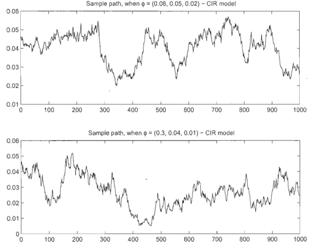
models, these percentages were 0 in both cases. Figure 2.1 shows, for each set ofparameters, the first simulated sample path of the Vasicek model, with n = 1000 observations.

A similar procedure is performed to generate two sets of trajectories for the

cm

pro­ cesses. Moreover, in the

cm

case we should also apply the condition 2Ke ~ 0-2 . Figure 2.2

shows, for each set of parameters, the first simulated sample path of the

cm

model, with n = 1000 observations.

The tables and figures in the next pages summarize the results of the simulation exer­ cise for the Vasicek and

cm

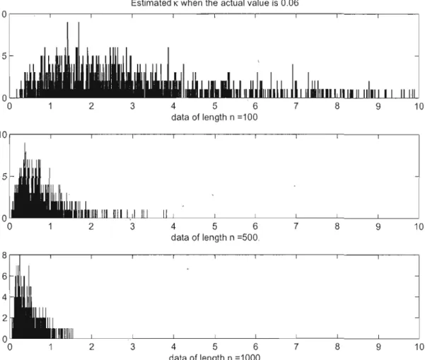
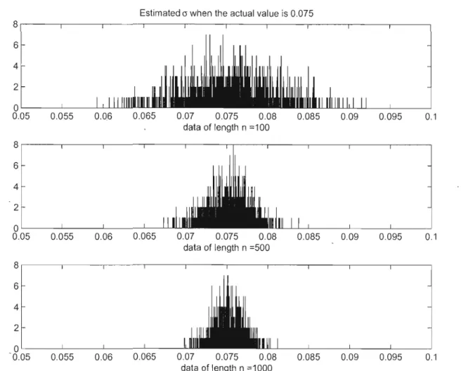
model using the maximum likelihood method. The plots for al! the results are outlined in Appendix A. The convergence of the estimated parameters to the true values as ri increases shows that the results are asymptotically unbiased.

Tables 2.1, 2.2, and 2.3 summarize the results of the simulation implementation with different numbers of observations. These tables include the true values, mean estimates over

N = 1000 simulations and the assodated standard deviations of the estimates. The mean provides the information about any bias in the estimation technique, while the standard deviation is useful in assessing the accuracy of the technique. Also we should mention that we observed outliers in results, especially when the number of observations was small. We used a box-and-whisker method to identify these outliers and ignore them afterwards in the computations.

Overall, based on the results, we might conclude that maximum likelihoodmethod is not a very successful method for determining the parameters. In the two next chapters we will study two different techniques.

Sample path, when <p = (0.06, 0.05, 0.02) - Vasicek model

0.2 r - - - - . , - - - - . . , - - - , - - - , - - - , . - - - , - - - , - - - , - - - - . - - - ,

0

0 100 200 300 400 500 600 700 800 900 1000

Sampie path, when <p = (0.3. 0.04, 0.01) - Vasicek model 0.06 0.05 0.04 0.03 0.02 0.01 0 100 200 300 400 500 600 700 800 900 1000

Sample path, when 4> = (0.06, 0.05, 0.02) - CIR model 0.06 ,---.,.---,---,----,---,---,---,,---,---.,.---, 0.05 0.04 0.03 0.02 0.01 '---_ _-L.-_ _--'----_ _---"---_ _----'---_ _---'-_ _---'- '---'--_-'---_ _--'---_---.J

o

100 200 300 400 500 600 700 800 900 1000

Sample path, when 4>

=

(0.3,0.04,0.01) - CIR model

0.06,---,----,---,---r---,---,--,---.---.,.----,---, 0.05 0.04 0.02 0.01 O'---L.---'---"---'---'---'----L---L.---'---.J

o

100 200 300 400 500 600 700 800 900 1000

Estimaled K when Ihe actual value is 0.06 10 r - - , - - - , - - - , - - - , - - - , , - - - , . - - - - , - - - , - - - - , . - - - , - - - , 5 2 3 4 5 6 7 8 9 10 dala of length n =100 10 r - - - - , - - - , - - - - , - - - , , - - - - , . - - - - , - - - , - - - , - - - , - - - , 4 5 6 7 8 9 10 data of lenglh n =500. 8 r - - r - - , . - - - , - - - r - - - , - - - , - - - , - - - . - - - - , - - - - , . - - - , 2 3 4 5 6 7 8 9 10 data of length n =1000

Estimated K when the actual value is 0.25 30 ,---,---,---,.---,-~-_,.---.___--___._--___r---...__--_, 20 10 2 3 4 5 6 7 8 9 10 data of length n =100 1 0 , - - - , - - - , - - - , - - - - , - - - r - - - r - - - r - - - , - - - , - - - , 5 2 3 4 5 6 7 8 9 10 data of length n =500 8 - - - , , . . . - - - , . . . - - - , - - - , - - - , , - - - . - - - , - - - r - - - , - - - , - - - , 2 3 4 5 6 7 8 9 10 data of length n =1000

5

o

'---'---_'---'JIJ

o

0.01 0.02 0.03 0.04 0.05 0.06 0.07 0.08 0.09 0.1

data of I.ength n =1000

Estimated (J when the actual value is 0.075 8 r - - - , . . - - - . - - - , - - - - r - - - . , - - - . - - - , - - - - , - - - , . . - - - , 6 4 2 O'--_ _...J..-_ _L-'---L.L..Luuu... 0.05 0.055 0.06 0.065 0.07 0.075 0.08 0.085 009 0.095 0.1 data of length n ::: 100 8 , - - - , - - - , - - - , - - - , , - - - T T - - - , - - - , - - - , - - - , - - - , 6 4 2 O'----..J...---'---'---...L.J...J... 0.05 0.055 0.06 0.065 0.07 0.075 0.08 0.085 0.09 0095 0.1 data of length n :::500 8 , - - - , . . - - - . - - - , - - - - , - - - - , - - - , - - - , - - - , , - - - , - - - , 6 4 2 -8.05 0.055 0.06 0.065 0.07 0.075 0.08 0.085 0.09 0.095 0.1 data of length n :::1000

Table 2.1 A simulation analysis of the MLEs with

n

=

100 observations

Vasicek

cm

Parameters Actual' Mean Standard Actual Mean Standard values estimates deviations values estima tes deviations

KI 0.060 3.182 2.337 0.250 3.126 2.360 K2 0.300 3.409 2.492 0.450 3.299 2.414

8

1 0.050 0.052 0.020 0.050 0.047 0.019

8

2 0.040 0.044 0.009 0.030 0.036 0.016 al 0.020 0,020 0.000 0.050 0.050 0.004 a2 0.010 0.010 0.000 0.075 0.075 0.005

Table 2.2 A simulation analysis of the MLEs with ft = 500 observations

Vasicek

cm

Parameters Actual Mean Standard Actual Mean Standard values estimates deviations values estimates deviations

KI 0.060 0.746 0.537 0.250 0.803 0.544 KZ 0.300 0.860 0.540 0.450 0.933 0.508

el

0.050 0.077 0.029 0.050 0.049 0.023

e

z 0.040 0.040 0.008 0.030 0.029 0.009 (JI 0.020 0.019 0.000 0.050 0.050 0.001 (Jz 0.010 0.010 0.000 0.075 0.075 0.002

Table 2.3 A simulation analysis of the MLEswith n

=

1000 observations

Vasicek

cm

Parameters Actual Mean Standard Actual Mean Standard values estimat~s deviations values estimates deviations

KI 0.060 4.271 0.271 0.250 0.516 0.287 K2 0.300 0.055 0.282 0.450 0.676 0.296 81 0.050 0.082 0.027 0.050 0.048 0.016 82 0.040 0.041 0.006 0.030 0.028 0.006 (JI 0.020 0.020 0.000 0.050 0.050 0.001 (J2 0.01'0 0.010 0.000 0.075 0.075 0.002

ZERO-COUPON DATA

3.1 Zero-coupon prices

Very often in finance we need to estima te the unknown parameter sets of state variables, when the random variates specified in the model are not directly observable. For example in the financial markets we can only see the priees of interest rate instruments, while we would need to know the interest rates (short rates in discrete time) for performing the estimation.

A different approach for the estimation Of the SDE-type models has been introduced in the financialliterature, by finding a function whieh de fines the relation between the ob­ servable data and the non-observable values, and then fitting this function to observable values (bond priees for example) at a specific period oftime.

In the literature, as discussed in Chapter II, the term structure of the interest rates, is assumed ta follow a diffusion process; Vasieek and CIR pro cesses are examples of this kind. However, these rates are not observable, butwe can use the affine term structure to relate the observable prices to unobserved state variables. In other words, we are interested in a model that is numerically and empirieally tractable, but sometimes the random variables of the model are not directly observable. For example, in our case the generated r(t) of the previous chapter doesn't exist in reality and can not be considered an instantaneous interest rate. However, the available data (such as bond prices) are often the result of sorne transformation ofthese unobservable rates.

In this Chapter, we develop a maximum likelihood rriethod for dealing "vith parameter estimation of zero-coupon interest rates which is an example of a problem of this type. The first step is to establish sorne relation between interest rates and the observable priees of the bonds, We denote the value (or priee) of a risk-free-zero-coupon bond as the function

P(t, Tl where t refers to the current time, while the T represents the coupon's maturity date; therefore it is obvious that ti < T for i = l"." n where n is the number of periods left to the maturity date. The zero-coupon bond pays one unit of account to the holder at maturity date T (ti = T, i = n), in other word PtT, T) = 1.

Cox, Ingersoll and Ross (l985b) suggest the fqllovving relation between the priee of the zero coupon and the continuous associated data, spot rate of interest, which is denoted by

z(t, T): P(t, T) = exp(-(T - t)z(T, t)) that is, logP(t, Tl z(t, Tl = - . T-t

Thus, z(t, T) can be regarded as a risk-free rate of interest in a fixed period of time T - t. The short rate is the spot interest rate "vith instantaneous maturity, Le.

r (t) = Hm z(t, Tl.

T-l

and from the above equation we have

. {logp(t, T) } r(t) = lim z(t, T) = hm ~--='----T~l T-l T- t = _ [àIOgp(t, T)] àT T=l = [ l àP(t, Tl ] Ptt, T) àT T=l = àP(ti t) àT

The affine term structure model is a key proeedure for calculating the zero-coupon rate from a given time to maturity, ptt, T), by having only the value of the instantaneous rate

on interest, r(t). We consider a class of models, called exponential affine, where the priees {P( t, T), tE: [0, Tl} are of the following general form:

pu, T) = eA(t,T)-'B(t,T)r(l) _(3.1.1)

with deterministic functions AU, T) and B(t, T). Since PtT, T) = 1, we should have the fol­ lowing boundary conditions:

A(T, T)

=

0, B(T, T)

=

o.

In the next sections we will describe the single-factor development of the above affine term structure model, and th en generalize it to higher dimensions (multi-factor models).

3.2 Single-factor models

Vasicek (1977) assumes that r(t) follows the SDE (Z.2.6), and uses this process and the as­ sumption of a constant market priee risk, A, to derive a bond pricing modellike (3.1.1) for

T - T - t, where, BU, T) = B(T) =

.!.

(1-

e-

KT ), x y(B(T)-T) (J2B 2(T) AU, T)

=

A(.)

=

x2 - 4x ' (3.2.Z) with

Let us denote

cp

= (x, e, (J) the vector of unknown parameters, T

=

T - t, the time to maturity (T

=

T - t is usually considered as a weekly, monthly or yearly point of observation).

Manyauthors use the Vasicek model in their pricing models, although there are many others who prefer to work with the model suggested by Cox, Ingersoll and Ross (1985b). The exponential affine formula (3.1.1) is still valid with A and B given by

Z(eYT - 1) B(~=

,

(y + x + A)(eYT - 1) +Zy AlT Zye (Y+<2+ ) 2;f A(T) = ln , (3.2.3) (

_(1.

_{+ x +} A)(eYT - 1) +Zy

and

The complete calculation for finding A and B in the single factor model for both Vasicek and

cm

processes is done in Bolder (2001).

3.3 Muiti-factor modeis

In these models one assumes that the short rate is in fact a linear combination of N corre­

lated state variable (factors) which we denote by YI, Y2,"" YN. Therefore, we have the follow­ ing equation,

N r(t)

=

LYi(t),

i=1

and the associated price function is,

p(t, Tl = p{t,T; YI, .. ·, YN)

= ,

exp { A(t, T)

-~

B;(t, T)Yi(t) } .

According to Bolder (2001), we have the following solution for the Vasicek model with:

and

By comparing the above equation with the single-factor case (3.2.2), we realize that, in addi­ tion to replacing the right-hand side in (3.2.2) with a sum of N terms, we also have an extra covariance term.

However, in the

cm

multi-factor model, things get more difficult and the analytical so­ lution exists only when the Ricatti equation arising from the partial differential equation (the

so-called term structure equationl can be reduced to independent one-dimensional equa­ tions, which implies that the underlying Browriian motions, Wj, ... ,WN are independent. In a similar way, the solution to the N-factor

cm

partial differential equation has the form

pu, Tl = PU, T; YI, ... ,Yn)

exp {

~

AiU, Tl - BiU, T)YiU) } (3.3.5) where

and the Brownian motions are independent. Again, the function AiU, T) and BiU, T) are of the same form as in the one-dimensional case, since we assume that the state variables are not correlated (in Chapter l, we also assumed that Wj , .•. ,W_n were independent); this gives

2(eYiT - 1)

Bi (T) = - - - ­

(Yi +Ki +

;U(e

YiT _{-1) +2Yi'}

(3.3.6)

where

Y· 1

=

V(K'

I i i ' +/1..)2 +20'2

In both cases the boundary conditions for i

=

l, ... ,N, are defined as

According to Bolder (2001), the previous derivation of continuous-time affine term structure models exists also for the discrete-time classes.

The theoretical development required to represent the bond priees as an affine func­ tion of the underlying state variables of the two specifie Vasicek and

cm

models is completed and we can introduce techniques to estimate the unknown parameters of the affine term­ structure models. In this Chapter we will only describe the maximum likelihood approach, and leave the Kalman flUer methodology for the next Chapter.

3.4 Maximum likelihood estimation

We view equation (3.1.1), as a transform function which relates short rates to zero-coupon priees:

rU) 0-+ pet, T)

=

eAlt.T)-B(I,T)r(t).

For 0 = ta < tl < ... < tn and a fixed set of parameters, we can then derive an inverse relation:

(3.4.7)

To obtain the log-likelihood function for the transformed data, we employ the following clas­ sic theorem.

Theorem 2 If the transformation from X to Y is on an element-by-element basis, i.e., Yi =

Ti(xi;cf»for all

i,

then

where

The proof of this theorern can be found in Duan (1994). In our specifie case. T(X, cf» rep­

resents the pricing function (3.1.1) and T-l will be the equation (3.4.7). Therefore, we can calcula te the log-likelihood function for the priees bond.

n A A ~l làP(Xi(cf>);cf>) 1

{(PU}, T),,,,, PUn,T); cf»

=

drUIl."., rUn); cf» - L. og ..

i=l àx ,

n

= ((fUI), ".,fUn); cf» -

L

10gIBUi,T)I (3.4.8)

i=l

where {(fUll,,,,, _{f(tn); cf» is in fact the calculated log-likelihood function for the Vasicek (or}

cm

model) in the previous chapter. The minimization of minus the log-likelihood function (3.4.8) can be achieved by the fminsearch function in MATLAB.

3.5

Numerical

analysis

In this section, to illustrate our method, we apply the preceding theoretieal discussion to the previous Chapter generated data, and apply equation 3.1.1 to collect the observable priees related to these instantaneous unobservable short rates (in reality).

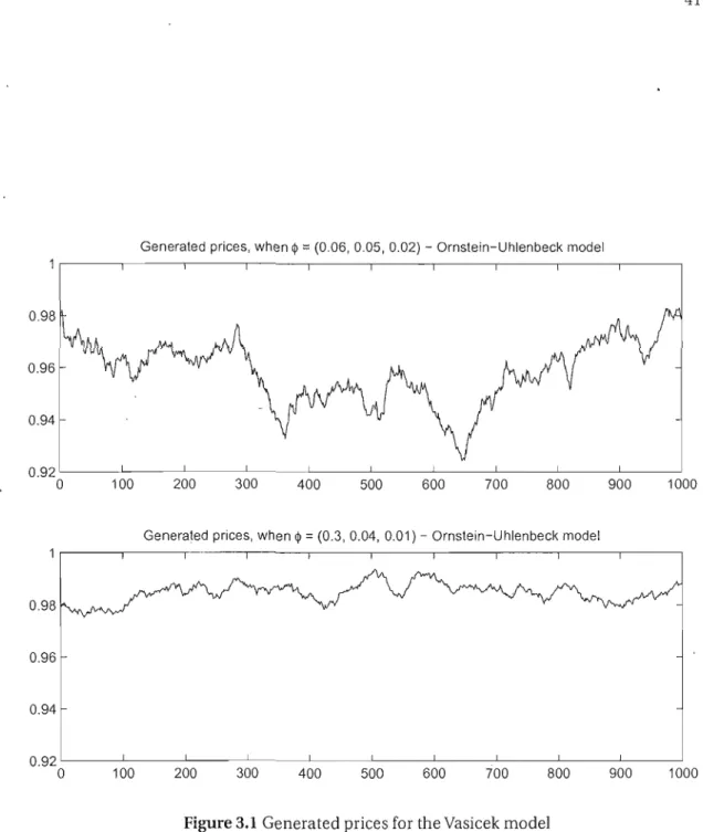
In particular, we compute these values by using weekly observations (6

=

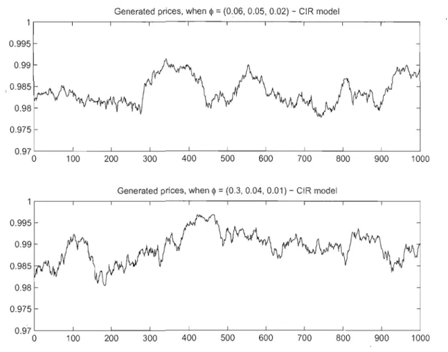
1/52) over a 20-year time horizon. The generated priees illustration for a lO-year zero-coupon bond (r

=

0.5) using Vasieek and

cm

models with the assumption of a constant risk premium

It = 1 are shown in figures 3.1 and 3.2 respectively.

Then we assume that the only data we have is the set of observed prices and use the inverse equation (3.4.7) to achieve estimation of short rates. By computing To, ... , Tn from

Po, ... ,Pn starting with an initial value <Po and applying the maximum likelihood method to

the log-likelihood function of priees (3.4.8), we can estima te the parameters of our mode!, the vector <Ji = (K,

e,

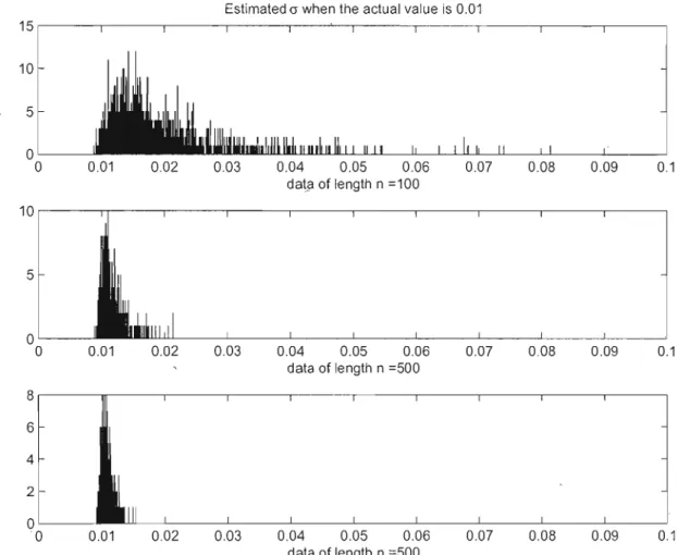
al The tables and figures in the following pages summarize the results

qf the simulation exercise for the Vasicek and

cm

models using the maximum likelihood method with zero-coupon prices. The plots of all the results are outlined in Appendix B.

The convergence of the estimators to the true values n increases shows that the results are asymptotieally unbiased. Tables 3.1, 3.2, and 3.3, summarize the results of the simula­ tion implementation with different numbers of observations. The estimators in the indirect method tend to the real values but the convergence is slow. Since in this method we are not directly getting the maximum likelihood estimates of the short rates, we were expecting to get these results.

Generaled priees, when q> = (0.06. 0.05, 0.02) - Ornslein-Uhlenbeek model 0.98 0.96 0.94 0.92 '---_ _-'----_ _--L-_ _---'---_ _---'--_ _----'-_ _---.1. '---_ _-'---_ _-'----_ _

o

100 200 300 400 500 600 700 800 900 1000

Generaled priees, when q> = (0.3, 0.04, 0.01) - Ornslein-Uhlenbeek model

0.98

0.96

0.94

0.92 '---_ _--L..-_ _- ' -_ _----'- L -_ _--'----_ _---'--_ _---,-' - ' - - -_ _--'----_ _---.J

o

100 200 300 400 500 600 700 800 900 1000

Generated priees, when Ql

=

(0.06, 0.05, 0.02) - CIR model 0.995 099 0.975 0.97 0 100 200 300 400 500 600 700 800 900 1000

Generated priees, when Ql = (0.3,0.04,0.01) ­ CIR model

0.995 0.99 0.985 0.98 0.975 0.97 0 100 200 300 400 500 600 700 800 900 1000

5

Estimated K when the actual value is 0.3