Quantitative WD-XRF calibration for small ceramic samples and their source material

Open Archive TOULOUSE Archive Ouverte (OATAO)

OATAO is an open access repository that collects the work of Toulouse researchers and

makes it freely available over the web where possible.

This is an author-deposited version published in :

http://oatao.univ-toulouse.fr/

Eprints ID : 11501

To link to this article : doi:10.1002/gea.20353

URL :

http://dx.doi.org/10.1002/gea.20353

To cite this version : De Vleeschouwer, François and Renson, Virginie

and Claeys, Philippe and Nys, Karin and Bindler, Richard Quantitative

WD-XRF calibration for small ceramic samples and their source

material. (2011) Geoarchaeology, vol. 26 (n° 3). pp. 440-450. ISSN

0883-6353

Any correspondance concerning this service should be sent to the repository

administrator:

staff-oatao@listes-diff.inp-toulouse.fr

Quantitative WD-XRF Calibration for

Small Ceramic Samples and Their

Source Material

François De Vleeschouwer,

_{* Virginie Renson,}

Philippe Claeys,

_{Karin Nys,}

_{and Richard Bindler}

1_{Department of Ecology and Environmental Sciences, Umeå University, SE-901}

87 Umeå, Sweden

2_{EcoLab UMR 5245 CNRS-UPS-INPT, Avenue de l’Agrobipole BP 32607,}

Auzeville tolosane, 31326, Castanet-Tolosan, France

3_{Earth System Science, Department of Geology, Vrije Universiteit Brussel,}

Pleinlaan 2, 1050 Brussels, Belgium

4_{Mediterranean Archaeological Research Institute, Vrije Universiteit Brussel,}

Pleinlaan 2, 1050 Brussels, Belgium

A wavelength-dispersive X-ray fluorescence (WD-XRF) calibration is developed for small pow-dered samples (300 mg) with the purpose of analyzing ceramic artifacts that might be available only in limited quantity. This is compared to a conventional calibration using a larger sample mass (2 g). The comparison of elemental intensities obtained in both calibrations shows that the decrease in analyzed sample mass results in a linear decrease in measured intensity for the analyzed elements. This indicates that the small- and large-sample calibrations are compara-ble. Moreover, the elemental contents of four ceramic sherds and two potential clay sources fall well within the range of the certified reference materials that are the basis of the calibra-tion curves. The advantage with the analytical method presented here is that it is rapid and requires only a small amount of sample that can easily be re-used for further analyses. This method has great potential in ceramic provenance studies. © 2011 Wiley Periodicals, Inc.

INTRODUCTION

In archaeometry a wide range of chemical techniques has been used to assess the geochemical content of various archaeological objects (e.g., Adan-Bayewitz, Asaro, & Giaque, 1999; Szökefalvi-Nagi et al., 2004; Asaro & Adan-Bayewitz, 2007; Cultrone et al., 2010; Mazar et al., 2010; Renson et al., 2011). Among these objects are ceramic sherds, which, if accurately quantified for their elemental content and analyzed in a multivariate statistical approach, can provide information on the source and trad-ing of ceramics in ancient times. The main problem of analyztrad-ing archaeological objects is that, for conservation reasons, the availability of sample is often limited. In the case of ceramics, the sample often consists of small fragments found on archaeological sites or retrieved from collections. Archaeometrists are therefore in

constant search for analytical techniques that allow elemental quantification on a min-imum amount of material.

X-ray fluorescence (XRF) is an analytical technique that has been widely used in many industrial, environmental, geological, and archaeological investigations (see West et al., 2010, for a recent review of XRF applications). Among the applications, XRF has been widely used in the earth sciences (e.g., Potts, 1987, and references therein; Gardner, 1990; Cheburkin, Frei, & Shotyk, 1997; Zambello & Enzweiller, 2002; West et al., 2010, and references therein) and has been developed to analyze vegetation samples (e.g., Cheburkin & Shotyk, 1996; Margui, Hidalgo, & Queralt, 2005) and liquid matrices (e.g., Cumming & McDonald, 1985; Varga et al., 1995; Oprea et al., 2009). In archaeological studies, XRF has a wide range of applications, and sam-ples can be potentially re-used for further analysis depending on the sample prepa-ration (e.g., Adan-Bayewitz, Asaro, & Giaque, 1999; Hein et al., 2004; Craig et al., 2007; Tripathi & Rajamani, 2007; Cultrone et al., 2010; West et al., 2010, and references therein). The common drawbacks of XRF are the so-called matrix effects, which are principally caused by the composition, grain size, and mineralogy of the sample. A way to minimize these effects is to finely powder the samples and to apply sub-sequent pretreatments such as lithium borate fusion or pelletization using a wax binder (Potts, 1987). However, these processes alter the properties of the samples, which then cannot be re-used for further analyses. Classical XRF on powder, pellets, or fused beads also requires several grams of sample to achieve an accurate ele-mental quantification (e.g., Zambello & Enzweiller, 2002; Cultrone et al., 2010). This limits its application to archaeological artifacts that are available only in sufficiently large quantity. For small samples, direct analysis of powdered material would there-fore be generally preferred. Such an application needs to be carefully developed to provide accurate elemental quantification (Adan-Bayewitz, Asaro, & Giaque, 1999). New generations of wavelength-dispersive XRF (WD-XRF) offer the potential to decrease the quantity of material by carefully developing calibrations on samples as small as a few hundred milligrams. A common WD-XRF setup allows the deter-mination of major and selected trace elements without specific spectrometric design. In this short note we provide the details of a calibration that was purposely devel-oped for quantifying selected elements in small ceramic fragments and their poten-tial raw materials. We present some of the technical aspects of the selection and preparation of the certified reference materials (CRMs) as well as a specific calibra-tion developed to optimize WD-XRF for ceramic matrices and their source materials. This specific calibration for small sample mass (300 mg) is validated by comparing the intensities obtained with a conventional calibration (i.e., using 2-g samples).

METHODOLOGY

Selection of Certified Reference Materials

Thirty-five commercially available CRMs were selected from our laboratory stock. All our CRMs are finely powdered and stored in desiccators. They consist of sedi-mentary and igneous rocks (NIST1d, NIST70a, NIST278, NIST2780, NIST688), river

sediments (NIST8704, STSD3), lake sediments (LKSD1, LKSD4, BIL1, JLK1), estuar-ine sediments (NIST1646a), and marestuar-ine sediments (NIST1944, NIST2702, NIST2703, MAG1, PACS2, MESS3) as well as sands (NIST81a, NIST1413), clays (NIST97b, NIST98b, NIST679), and soils (SO2, SO3, SO4, NIST2711, NIST2586, NCSDC73325, NCSDC73326, JSO1) from sedimentary outcrops, and coal fly ash (JCFA1, NIST1633a, NIST1633b, ZUK1), the latter type being added to extend the range of various trace elements. Rather than exclusively choosing fine sediments, we have included several sediment and rock types to represent mixed matrices (i.e., fine material and tem-per) that may be found in ceramics (Rapp, 2009).

Sample Preparation

All the analyses were carried out directly on CRM powders. Two calibrations were developed: one based on 2 g of each CRM, as commonly done in XRF analyses, and a second based on 300 mg of powder that was specifically developed here. For the first calibration, 2 g of dried and homogenized loose powder was transferred to 40-mm-opening plastic cups with a 2.5-mm transparent mylar film at its base. These samples were placed in 36-mm-opening metallic cup holders for analysis. The chal-lenging part of this study was the development of the second calibration, using 300 mg of powder, which was transferred to a plastic cup with a 10-mm opening, also with a 2.5-mm mylar film at the base. In these small cups the powder was slightly compressed manually to reduce porosity effects. These plastic cups were subsequently loaded in a metallic cup holder with an opening (i.e., analytical) diameter of 8 mm.

XRF Optimization

All the analyses were conducted using a Bruker S8-Tiger WD-XRF analyzer equipped with a Rh anticathode X-ray tube, four analyzing crystals (XS-55, PET, LIF200, LIF220), a flow proportional counter (for light elements), and a scintillation counter (for heavy elements). Analyses were performed under helium atmosphere to avoid powder loss in the analytical chamber, which may occur under vacuum conditions. The main param-eters, used for each calibration and each element, are reported in Table I. Such a WD-XRF setup allows the determination of a wide range of elements, generally from C to U. In this study, the following elements were selected: Na, Mg, Al, Si, P, S, K, Ca, Ti, V, Mn, Fe, Ni, Cu, Zn, Br, Rb, Sr, Ba, and Pb. This selection is based on the certified val-ues available in each CRM, which are matched with the expected detectable concen-trations of our WD-XRF spectrometer. The WD-XRF resolution and sensitivity have been optimized by combining the proper collimators, crystals, and counters for each element (Table I). The peak acquisition time was optimized using the built-in SpectraPlus®

soft-ware interface, which calculates the time necessary to achieve an average selected detection limit. The acquisition time varies, therefore, among elements as well as among concentrations of a given element (i.e., the lower the concentration, the greater the time). To avoid any excessively long acquisition times, a maximum time was set for each element, which varies from 30 to 100 s (Table I). The background measure-ment times have been fixed manually, generally at 10 s, except for a few trace elemeasure-ments

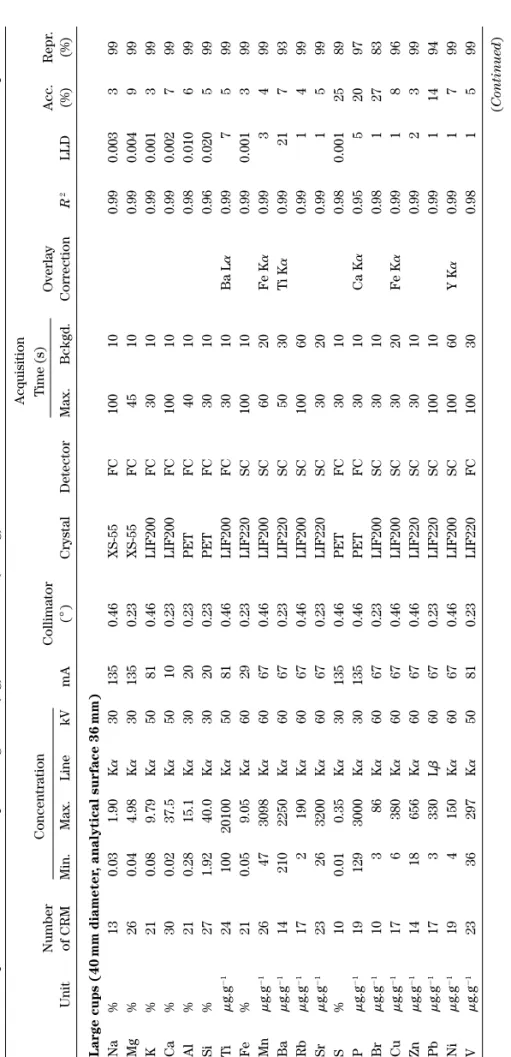
T

able I.

Main parameters used to develop both large mass (2

g) and small mass (300

mg) calibrations. The minimum and maximum CRM concentra

tions are also reported.

Acquisition Number Concentration Collimator T ime (s) Overlay Acc. Repr . Unit of CRM Min. Max. Line kV mA ( ° ) Crystal Detector Max. Bckgd. Correction R 2 LLD (%) (%) Large cups (40 mm diameter , analytical surface 36 mm) Na % 1 3 0.03 1.90 K a 30 135 0.46 XS-55 FC 100 10 0.99 0.003 3 9 9 Mg % 2 6 0.04 4.98 K a 30 135 0.23 XS-55 FC 45 10 0.99 0.004 9 9 9 K % 21 0.08 9.79 K a 50 81 0.46 LIF200 FC 30 10 0.99 0.001 3 9 9 Ca % 3 0 0.02 37.5 K a 50 10 0.23 LIF200 FC 100 10 0.99 0.002 7 9 9 Al % 2 1 0.28 15.1 K a 30 20 0.23 PET FC 40 10 0.98 0.010 6 9 9 Si % 2 7 1.92 40.0 K a 30 20 0.23 PET FC 30 10 0.96 0.020 5 9 9 Ti m g.g ⫺ 1 24 100 20100 K a 50 81 0.46 LIF200 FC 30 10 Ba L a 0.99 7 5 99 Fe % 2 1 0.05 9.05 K a 60 29 0.23 LIF220 SC 100 10 0.99 0.001 3 9 9 Mn m g.g ⫺ 1 26 47 3098 K a 60 67 0.46 LIF200 SC 60 20 Fe K a 0.99 3 4 99 Ba m g.g ⫺ 1 14 210 2250 K a 60 67 0.23 LIF220 SC 50 30 T i K a 0.99 21 7 9 3 Rb m g.g ⫺ 1 17 2 190 K a 60 67 0.46 LIF200 SC 100 60 0.99 1 4 99 Sr m g.g ⫺ 1 23 26 3200 K a 60 67 0.23 LIF220 SC 30 20 0.99 1 5 99 S % 10 0.01 0.35 K a 30 135 0.46 PET FC 30 10 0.98 0.001 25 89 P m g.g ⫺ 1 19 129 3000 K a 30 135 0.46 PET FC 30 10 Ca K a 0.95 5 2 0 9 7 Br m g.g ⫺ 1 10 3 8 6 K a 60 67 0.23 LIF200 SC 30 10 0.98 1 2 7 8 3 Cu m g.g ⫺ 1 17 6 380 K a 60 67 0.46 LIF200 SC 30 20 Fe K a 0.99 1 8 96 Zn m g.g ⫺ 1 14 18 656 K a 60 67 0.46 LIF220 SC 30 10 0.99 2 3 99 Pb m g.g ⫺ 1 17 3 330 L b 60 67 0.23 LIF220 SC 100 10 0.99 1 1 4 9 4 Ni m g.g ⫺ 1 19 4 150 K a 60 67 0.46 LIF200 SC 100 60 Y K a 0.99 1 7 99 V m g.g ⫺ 1 23 36 297 K a 50 81 0.23 LIF220 FC 100 30 0.98 1 5 99 (Continued )

T able I. (Continued ) Acquisition Number Concentration Collimator T ime (s) Overlay Acc. Repr . Unit of CRM Min. Max. Line kV mA ( ° ) Crystal Detector Max. Bckgd. Correction R 2 LLD (%) (%) Small cups (10 mm diameter , analytical surface 8 mm) Na % 1 0 0.01 1.59 K a 30 135 0.46 XS-55 FC 100 30 0.99 0.007 5 9 2 Mg % 2 1 0.04 4.98 K a 30 135 0.23 XS-55 FC 30 20 0.99 0.009 7 9 3 K % 19 0.08 3.45 K a 50 81 0.23 LIF200 FC 30 10 0.99 0.002 3 9 0 Ca % 2 6 0.02 15.0 K a 50 10 0.23 LIF200 FC 100 10 0.99 0.005 7 9 0 Al % 1 0 0.28 6.42 K a 30 20 0.23 PET FC 180 10 0.98 0.010 7 9 1 Si % 2 4 1.92 40.0 K a 30 20 0.23 PET FC 30 10 0.96 0.030 4 9 0 Ti m g.g ⫺ 1 25 100 14300 K a 50 81 0.46 LIF200 FC 100 10 Ba L a 0.99 13 5 9 2 Fe % 2 1 0.05 9.05 K a 50 5 0.23 LIF220 SC 100 10 0.99 0.010 4 9 2 Mn m g.g ⫺ 1 25 47 3098 K a 60 67 0.46 LIF200 SC 100 60 Fe K a 0.99 4 5 92 Ba m g.g ⫺ 1 10 180 1490 K a 60 67 0.23 LIF220 SC 100 60 T i K a 0.99 114 9 9 1 Rb m g.g ⫺ 1 18 2 190 K a 60 67 0.46 LIF200 SC 100 60 0.97 1 1 1 9 3 Sr m g.g ⫺ 1 21 26 1041 K a 60 67 0.23 LIF220 SC 100 60 0.99 2 9 93 S % 19 0.01 1.57 K a 30 135 0.46 PET FC 30 10 0.80 0.002 36 99 P m g.g ⫺ 1 22 129 1279 K a 60 135 0.46 PET FC 30 10 Ca K a 0.72 202 26 88 Br m g.g ⫺ 1 8 3 86 K a 60 67 0.23 LIF200 SC 100 60 0.98 1 2 7 4 7 Cu m g.g ⫺ 1 16 6 310 K a 60 67 0.46 LIF200 SC 100 60 Fe K a 0.99 2 4 78 Zn m g.g ⫺ 1 26 18 414 K a 60 67 0.46 LIF200 SC 100 60 0.97 3 1 0 9 1 Pb m g.g ⫺ 1 9 1 2 330 L b 60 67 0.23 LIF220 SC 100 60 0.99 5 4 88 Ni m g.g ⫺ 1 17 8 150 K a 60 67 0.46 LIF200 SC 300 60 Y K a 0.99 1 8 82 V m g.g ⫺ 1 19 36 297 K a 50 81 0.23 LIF220 FC 150 60 0.99 4 3 90

Kv: kilovolts; mA: milli-amperes; XS-55: W/Si multilayer crystal; LIF200 and 220: lithium fluoride crystals; PET

: pentaerythrit

e crystal; LLD: lower limit of detection. The accuracy (Acc.)

is the median value obtained by comparing the CRMs and the corrected XRF concentrations for each element in each standard. The

reproducibility (Repr

.) is obtained by repeated

meas-urements (

n

⫽

where intensities were expected to be low (see Table I). The overall measurement time is about 40 min per sample (i.e., 36 samples/24 h).

The calibration procedure is achieved in two steps: (1) all the CRMs are scanned at standard conditions to allow for optimization of sensitivity, resolution, and detec-tion limits (see preceding), and then (2) a full analysis of the CRMs selected to give the best fit (i.e., to minimize standard error) of the ultimate calibration line is con-ducted. This necessary selection depends on (a) the available certified values; (b) the behavior of each CRM matrix in both calibrations (2 g loose powder vs. 300 mg pressed powder); and (c) the targeted standard error, which can be decreased by care-fully removing values slightly off the calibration line without changing its slope. This selection process explains why, for a given element, the number of CRMs may vary between both calibrations (Table I). A posteriori corrections are also applied. They are of two types: (1) a software-built matrix correction that takes into account the inter-elemental interferences in the sample (i.e., a fluorescence X-ray originating from an element that causes electronic transitions in elements with lower energies), and (2) overlay corrections that are applied individually for peak overlaps commonly encountered in XRF spectra (see Table I). Finally, a quantitative calibration curve has been developed for each element by using a linear regression between the corrected intensities and the CRM concentrations through the built-in software.

In addition, an in-house standard (STG) is measured daily to check the analytical performance of the XRF. Three additional internal standards (SQ1, SQ3, Ausmon) are used to monitor the long-term (yearly) drift of the device and to correct intensities if necessary. Lower limits of detections (LLD) are calculated as follows:

where S_iis the analytical sensitivity (Cps/concentration), I_bis the background inten-sity (in kilocounts per second, Cps), and T_bis the background measurement time (s). It is also possible to recalculate a corrected concentration for each CRM by plot-ting its corrected intensity on the calibration line. This value was used to monitor the total analytical accuracy for each CRM and each element as follows:

where CCRMis the certified concentration and Ccoris the corrected (i.e., recalculated)

concentration. Finally, reproducibility has been assessed for both calibrations using an external CRM (which is not included in the calibration process) with a similar matrix (NCS-ZC73002, soil). Multiple (n⫽ 10) runs of this CRM provide a repro-ducibility expressed as follows:

reproducibility Average Cn Stdeva Cn

(% )₌ ⫽10⫺ ⫽10 A Average C_n⫽10 ×100 Accuracy C C C CRM COR CRM = ( − ) ×100 2 LLD S I T i b b = 3

where Average and Stdeva represent the mean (n⫽ 10) CRM concentration and standard deviation, respectively. Results, as well as detection limits, accuracies, and reproducibilities are reported in Table I.

RESULTS AND DISCUSSION

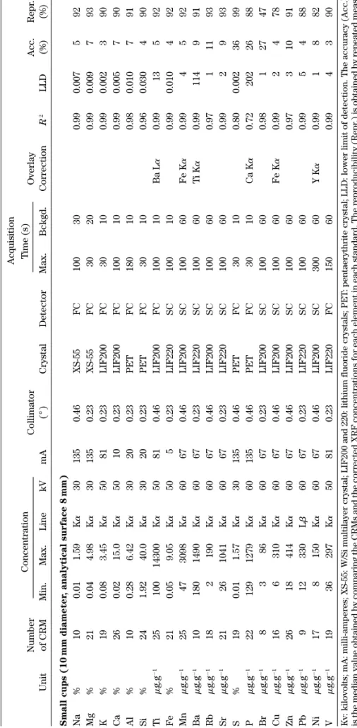
Potassium (K), titanium (Ti), zinc (Zn), and phosphorus (P) were chosen to illus-trate the comparison of the two calibrations and the reliability of the small-sample calibration. Potassium (major constituent) and Ti (minor constituent) were selected because they represent two important lithogenic elements commonly used in prove-nance studies. Zinc illustrates the behavior of heavy metals and phosphorus a cali-bration that displays greater uncertainty. Figure 1 presents biplots of the corrected intensities for both large-cup and small-cup calibrations. Because the number of CRMs for a given element differs between the large-cup and small-cup calibrations, only the intensities of the CRM common to each calibration are plotted together. For most of the studied elements, the CRM intensities plot nicely along a line (R2ⱖ

0.89 for elements in Figure 1), which indicates that decreasing the amount of mate-rial results in a linear decrease in the peak intensities. The intensities generally

0 0 1 2 3 4 5 6 K 7 20 40 60 Corrected intensity (kCps) 2g Calibration 80 100 120 Corrected intensity (kCps) 300mg Calibration 0 0 0.5 1 1.5 2 2.5 3 Ti 3.5 4 4.5 10 20 30 Corrected intensity (kCps) 2g Calibration 40 50 60 70 80 90 Corrected intensity (kCps) 300mg Calibration 0 0 0.1 0.2 0.3 0.4 0.5 0.6 Zn 0.7 20 40 60 Corrected intensity (kCps) 2g Calibration 80 100 120 140 Corrected intensity (kCps) 300mg Calibration 0 0 0.1 0.2 0.3 0.4 P 2 4 6 Corrected intensity (kCps) 2g Calibration 8 10 1 3 5 7 9 11 Corrected intensity (kCps) 300mg Calibration y⫽0.0543x ⫺ 0.0232 R2⫽_0.99 y⫽0.048x ⫹ 0.0085 R2⫽_0.99 y⫽0.0493x ⫹ 0.0168 R2⫽_0.99 y⫽0.0394x ⫺ 0.0182 R2⫽_0.89

Figure 1.Biplot comparison of intensities (kilocounts per second—kCps) obtained using the large and the small calibrations for K, Ti, Zn, and P. Black dots represent the CRMs.

decrease by a factor 15 to 25 from the 2-g to the 300-mg samples. However, both elemental peak and background intensities decrease, allowing for a good peak– background resolution. This is also supported by the low and comparable LLD found in both calibrations: a few tens of mg g⫺1_{and a few mg g}⫺1_{for major and trace elements,}

respectively (Table I). These values are generally below or equal to previously reported data (Cheburkin, Frei, & Shotyk, 1997; Boyle, 2000; Hein et al., 2002; Zambello & Enzweiller, 2002; Cultrone et al., 2010). Similarities between the two calibrations can also be observed for the accuracies, which remain within ⱕ10% for most elements except for S, P, and Br. These accuracy values are slightly below values encountered in the literature (Cheburkin, Frei, & Shotyk, 1997; Boyle, 2000; Zambello & Enzweiller, 2002; Cultrone et al., 2010). Improvements in both LLD and accuracy can be explained by the continuous analytical development of commercially available XRF and the care-ful selection of appropriate CRMs and WD-XRF optimization. Lower detection lim-its and accuracies have been reported by Adan-Bayewitz, Asaro, & Giaque (1999), who have used a specific Ag-cathode XRF setup. While such a configuration results in lower LLD and accuracies, it does not allow the determination of all major elements, which is crucial in provenance studies. Moreover, such a configuration is of limited availability compared to largely commercially available Rh-cathode WD-XRF. Compared to the large-cup calibration, reproducibility values are generally 5–10% lower for the small-cup calibration (Table I). This can be explained by the smaller analytical surface (8-mm vs. 36-mm opening), which results in a lower signal inte-gration. However, these reproducibilities are fully satisfactory, with values mostly above 90%, except for a very few elements (e.g., Cu: 78% and Ni: 82%). One notable exception is Br, which shows rather poor reproducibility (47%). This may be explained by (1) the low concentration encountered in the CRM analyzed for this test (2.8 mg g⫺1_{), (2) the relatively low amount of CRM with certified values for Br (n⫽ 8; see Table I),}

and (3) the low intensities (0–0.15 kilocounts per second) recovered for this ele-ment. Bromine concentrations should therefore not be taken as a fully quantified element using the small-cup calibration, but rather as indicative of large variations, which may be taken into account when using multivariate statistics, where covari-ance is considered rather than absolute values.

The linear relationship between the two calibration intensities also implies that results are independent of the calibration. In other words, the results of samples quantified with one calibration can be compared directly with the results obtained using the other. In the specific context of a provenance study, it is therefore possi-ble to compare source materials where a large amount of material is availapossi-ble, such as soils, rocks, and sediments, with small ceramic sherds (where the amount of material may be limited) using the two different calibrations based on the same CRM, but differing in the amount of material (2 g vs. 300 mg) and analytical surface (36 mm vs. 8 mm). Both major and trace elements display linear behaviors similar to K, Ti, and Zn, with low intercept offsets. Two elements display poor agreement: P and Ba. However, it should be noted that these two elements can be accurately quanti-fied using the large-cup calibration. The comparison between the two calibrations is poor because P and Ba are inaccurately quantified using the small-cup calibra-tion. This can be explained by a narrow CRM concentration range for P and bad

peak–background ratios for P and Ba. Caution is therefore required when using these elements in ceramic provenance studies where their concentrations have been meas-ured with the technique described here. However, in provenance studies where multivariate statistical approaches are often used to identify pottery groups and provenances, the loss of two minor elements out of a total suite of 20 elements will not influence significantly the results of multivariate statistical calculations.

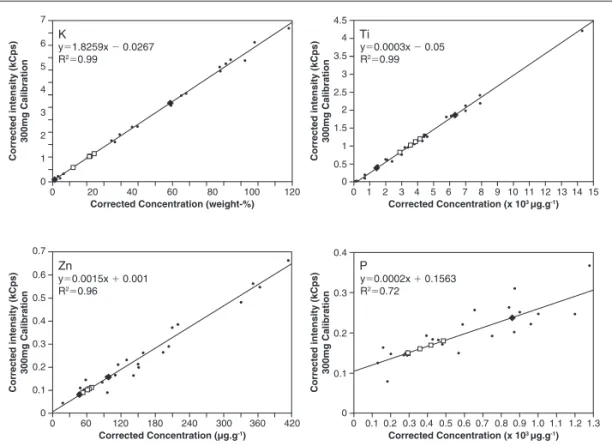
The small-cup calibration curves for K, Ti, Zn, and P are reported in Figure 2. To briefly illustrate the applicability of the small-cup calibration to ceramic artifacts, the elemental concentrations of four Cypriot Late Bronze age ceramic sherds and two potential raw materials have been measured; complete analyses of those samples will be presented in a separate publication. The concentration ranges found in the sherds and sediments are well enclosed within the CRM concentration ranges (Figure 2). As shown by the Zn biplots, trace metal concentrations are found to be relatively low in these sherds and sediments. This is also the case for the Pb concentrations (⬍15mg g⫺1, not shown here), which may potentially limit the applicability of XRF to trace metals in ceramic provenance studies. These considerations regarding elemental chemistry need, however, to be confirmed by the analysis of a wider range of ceramic

0 0 1 2 3 4 5 6 K 7 20 40 60

Corrected Concentration (weight-%)

80 100 120 Corrected intensity (kCps) 300mg Calibration 0 0 0.5 1 1.5 2 2.5 3 Ti 3.5 4 4.5 1 2 3 Corrected Concentration (x 103 _µg.g-1₎ 4 5 6 7 8 9 10 11 12 13 14 15 Corrected intensity (kCps) 300mg Calibration 0 0 0.1 0.2 0.3 0.4 0.5 0.6 Zn 0.7 60 120 180 Corrected Concentration (µg.g-1₎ 240 300 360 420 Corrected intensity (kCps) 300mg Calibration 0 0 0.1 0.2 0.3 0.4 P 0.2 0.4 0.6 Corrected Concentration (x 103 _µg.g-1₎ 0.8 1.0 0.1 0.3 0.5 0.7 0.9 1.1 1.2 1.3 Corrected intensity (kCps) 300mg Calibration y⫽1.8259x ⫺ 0.0267 R2_⫽0.99 y⫽0.0003x ⫺ 0.05 R2_⫽0.99 y⫽0.0015x ⫹ 0.001 R2_⫽0.96 y⫽0.0002x ⫹ 0.1563 R2_⫽0.72

Figure 2.Calibration lines (corrected intensities in kCps vs. CRM concentrations) obtained using the small cups for K, Ti, Zn, and P. Black dots represent the CRM. Open squares represent the pottery sherds. Black diamonds represent two potential raw materials from Cyprus.

artifacts in order to better explore the concentration range of each element using WD-XRF.

One last but major advantage of WD-XRF, besides providing quantitative data on a large amount of elements (here 18 to 20 elements), is that these same powdered samples can be re-used for further analyses such as mineralogy determination by X-ray diffraction, or isotopic analyses. The calibration developed here renders this re-use possible even on very small samples. It should finally be emphasized that while 300 mg of sample powder is sufficient, one should make sure that such a small amount is sufficiently representative of the whole object.

CONCLUSIONS

This study presents a rapid, non-destructive (i.e., the powdered samples can be re-used) WD-XRF protocol developed for small sample masses, down to 300 mg of dry powder. This protocol allows the accurate determination of major (Na, Mg, Al, Si, K, Ca, Fe), minor (Ti, P, S, Mn), and trace (V, Ni, Cu, Zn, Br, Rb, Sr, Ba, Pb) ele-ments. With the exception of three elements (P, Ba, Br), this specific calibration is fully comparable to conventional calibration using larger amounts of sample (2 g). Lower limits of detections and accuracies are comparable to, if not below, those found in the literature using similar XRF designs. Such a small sample calibration developed for pottery sherds may be widely applied in the field of ceramic provenance studies.

The WD-XRF acquisition, setup, and optimization was made possible through a research grant from the Kempe Foundation to R.B., which also provided a post-doc fellowship to F.D.V. Additional support was provided by the Research Foundation Flanders (FWO grants KN137 to K.N. and G.0585.06 to P.C.), the Research Council of the Vrije Universiteit Brussel (grant HOA11 to K.N. and P.C.), and the Swedish Research Council (grant to R.B.). We also thank Dr. Flourentzos, Director of the Department of Antiquities, Cyprus, for granting export permission for the sherds from Hala Sultan Tekke-Vyzakia. The comments of M. Kylander, A. Martinez-Cortizas, as well as two anonymous reviewers and editor G. Huckleberry improved an earlier version of this manuscript.

REFERENCES

Adan-Bayewitz, D., Asaro, F., & Giaque, R.D. (1999). Determining pottery provenance: Application of a new high-precision X-ray fluorescence method and comparison with instrumental neutron activation analy-sis. Archaeometry, 41, 1–24.

Asaro, F., & Adan-Bayewitz, D. (2007). The history of the Lawrence Berkeley National Laboratory instru-mental neutron activation analysis programme for archaeological and geological materials. Archaeometry, 49, 201–214.

Boyle, J.F. (2000). Rapid elemental analysis of sediment samples by isotope source XRF. Journal of Paleolimnology, 23, 213–221.

Cheburkin, A.K., & Shotyk, W. (1996). An energy-dispersive miniprobe multielement analyser (EMMA) for direct analyses of Pb and other trace elements in peats. Fresenius Journal of Analytical Chemistry, 354, 688–691.

Cheburkin, A.K., Frei, R., & Shotyk, W. (1997). An energy-dispersive miniprobe multielement analyser (EMMA) for direct analysis of trace and chemical age dating of single mineral grains. Chemical Geology, 135, 75–87.

Craig, N., Speakman, R.J., Popelka-Filcoff, R.S., Glascock, M.D., Robertson, J.D., Shackley, M.S., & Aldenderfer, M.S. (2007). Comparison of XRF and PXRF for analysis of archaeological obsidian from southern Peru. Journal of Archaeological Science, 34, 2012–2024.

Cultrone, G., Molina, E., Grifa, C., & Sebastián, E. (2010). Iberian ceramic production from Basti (Baza, Spain): First geochemical, mineralogical and textural characterization. Archaeometry, in press. DOI: 10.1111/j.1475-4754.2010.00545.x.

Cumming, G., & McDonald, I.G. (1985). The determination of iron in lubricating oils by X-ray fluores-cence spectrometry. Wear, 103, 57–66.

Gardner, L.R. (1990). Geochemical analysis of silicate rocks and soils by XRF using pressed powders and a two-stage calibration procedure. Chemical Geology, 88, 169–182.

Hein, I., Day, P.M., Cau Ontivreros, M.A., & Kilikoglou, V. (2004). Red clays from central and eastern Crete: Geochemical and mineralogical properties in view of provenance studies on ancient ceramics. Applied Clay Science, 24, 245–255.

Hein, A., Tsolakidou, A., Iliopoulos, I., Mommsen, H., Buxeda i Garrigós, J., Montana, G., & Kilikoglou, V. (2002). Standardisation of elemental analytical technique applied to provenance studies of archaeo-logical ceramics: An interlaboratory calibration study. The Analyst, 127, 542–553.

Marguí, E., Hidalgo, M., & Queralt, I. (2005). Multielemental fast analysis of vegetation samples by wave-length dispersive X-ray fluorescence spectrometry: Possibilities and drawbacks. Spectrochimica Acta Part B, 60, 1363–1372.

Mazar, E., Horowitz, W., Oschima, T., & Goren, Y. (2010). A cuneiform tablet from the Ophel in Jerusalem. Israel Exploration Journal, 60, 4–21.

Oprea, C., Maslov, O.D., Gustova, M.V., Belov, A.G., Szalanski, P.J., & Oprea, I.A. (2009). IGAA and XRF methods used in oil contamination research. Vacuum, 83, S162–S165.

Potts, P.J. (1987). A handbook of silicate rock analysis. Glasgow: Blackie & Son Limited. Rapp, G.R. (2009). Archaeomineralogy, 2nd ed. Heidelberg: Springer.

Renson, V., Coenaerts, J., Nys, K., Mattielli, N., Vanhaecke, F., Fagel, N., & Claeys, P. (2011). Lead isotopic analysis for the identification of Late Bronze Age pottery from Hala Sultan Tekke (Cyprus). Archaeometry, 53, 37–57.

Szökefalvi-Nagy, Z., Demeter, I., Kocsonya, A., & Kovács, I. (2004). Non-destructive XRF analysis of paint-ings. Nuclear Instruments and Methods in Physics Research Section B: Beam Interactions with Materials and Atoms, 226, 53–59.

Tripathi, J.K., & Rajamani, V. (2007). Geochemistry and origin of ferruginous nodules in weathered gran-odioritic gneisses, Mysore Plateau, southern India. Geochimica et Cosmochimica Acta, 71, 1674–1688. Varga, K., Hunyadi, I., Hakl, J., Uzonyi, I., & Bacsû, J. (1995). Gross alpha radioactivity and chemical trace element content of thermal waters measured by SSNTD and XRF methods. Radiation Measurements 25, 577–580.

West, M., Ellis, A.T., Potts, P.J., Streli, C., Vanhoof, C., Wegrzynek, D., & Wobrauschek, P. (2010). Atomic spectrometry update—X-ray fluorescence spectrometry. Journal of Analytical Atomic Spectrometry, 25, 1503–1545.

Zambello, F.R., & Enzweiler, J. (2002). Multi-element analysis of soil and sediments by wavelength-dispersive X-ray fluorescence spectrometry. Journal of Soils and Sediments, 2, 29–36.

GEOARCHAEOLOGY: AN INTERNATIONAL JOURNAL, VOL. 26, NO. 3 450