Any correspondence concerning this service should be sent to the repository administrator:
[email protected]
To link to this article:
DOI:10.1109/TUFFC.2009.1340
http://dx.doi.org/10.1109/TUFFC.2009.1340
This is an author-deposited version published in:
http://oatao.univ-toulouse.fr/
Eprints ID: 8050
To cite this version:
Nadal, Clément and Pigache, François Multimodal electromechanical model of
piezoelectric transformers by Hamilton's principle. (2009) IEEE Transactions on
Ultrasonics, Ferroelectrics and Frequency Control, vol. 56 (n° 11). pp.
2530-2543. ISSN 0885-3010
O
pen
A
rchive
T
oulouse
A
rchive
O
uverte (
OATAO
)
OATAO is an open access repository that collects the work of Toulouse researchers and
makes it freely available over the web where possible.
Abstract—This work deals with a general energetic
ap-proach to establish an accurate electromechanical model of a piezoelectric transformer (PT). Hamilton’s principle is used to obtain the equations of motion for free vibrations. The modal characteristics (mass, stiffness, primary and secondary electro-mechanical conversion factors) are also deduced. Then, to il-lustrate this general electromechanical method, the variational principle is applied to both homogeneous and nonhomogeneous Rosen-type PT models. A comparison of modal parameters, mechanical displacements, and electrical potentials are pre-sented for both models. Finally, the validity of the electro-dynamical model of nonhomogeneous Rosen-type PT is con-firmed by a numerical comparison based on a finite elements method and an experimental identification.
I. Introduction
T
he emergence of piezoelectric transformers coincides with the development in the 1950s of ferroelectric ceramics belonging to the perovskites crystalline family. The first architecture was proposed by rosen [1], who designed a step-up piezoelectric transformer (PT) made in barium titanate (baTio3) rod in 1956. In addition to providing small size and weight, PTs offer outstanding performance in terms of galvanic insulation, voltage ratio, and efficiency. Furthermore, compared with conventional electromagnetic transformers, PTs are free from electro-magnetic interference. They are consequently more suit-able for low-power applications, high efficiency, and small embedded systems.For some years, a wide range of piezoelectric trans-former structures has been developed to ensure various electrical requirements, also considering fixed constraints or environmental conditions. substantial performance im-provements have been reached with the development of new piezoactive materials and manufacturing process.
Typically, PTs provide optimal performances when they are supplied by voltage power supply close to one of their mechanical resonance frequencies. Furthermore, these frequencies depend strongly on dimensions, shape, and mechanical properties of the medium. This implies that vibratory eigenmodes must be clearly defined and
convenient models have to describe the electromechanical behavior. The development of analytical models [2]–[3] is particularly suitable for implementation into optimization algorithms [4] to deduce optimal dimensions.
The present paper relies on the development of a gen-eral analytical method to treat the modeling of any PT for several vibratory modes. With this analytical multimodal approach, the performance can also be predicted for dif-ferent kinds of PT design.
First, the general method based on Hamilton’s principle and matrix formulation is detailed. Then, this method is illustrated by modeling a classical rosen-type transformer with consideration of nonhomogenous electromechanical properties along the displacement axis. The same method is also used for this transformer considering a current ap-proximation of a homogenous elastic medium. as result, both problem formulations are balanced and thus highlight the influence of this assumption in terms of precision.
Finally, the modal parameters (i.e., the modal mass, the modal stiffness, the transformer ratio, the resonant frequency at shorted circuit) will be extracted and com-pared with those that come from a numerical study using a finite elements method and an experimental identifica-tion.
II. General analytical Formulation
Following the example of conventional magnetic trans-formers, the piezoelectric transformers are composed of primary and secondary sections with the difference that the coupling lies in an electromechanical conversion. The transformer is driven by a sinusoidal voltage power supply. The frequency of applied voltage usually coincides with a fundamental mode of vibration to take advantage of the best electrical performances of the PT (efficiency, voltage step-up ratio).
To establish a multimodal model of any piezoelectric transformer, a general analytical formulation is presented in following sections. First, the Hamilton’s principle is de-tailed, governed by matrix formulation. Then, a method-ology to deduce modal shapes is undertaken to get to the electromechanical model.
A. Electromechanical Modeling
To access the electromechanical behavior of the PT, an energy approach based on Hamilton’s principle seems to
Multimodal Electromechanical Model of
Piezoelectric Transformers by
Hamilton’s Principle
clement nadal and Francois PigacheThe authors are with the Universite de Toulouse; InP, UPs; lab-oratoire Plasma et conversion d’Energie (laPlacE); Ecole nation-ale supérieure d´Electrotechnique, d´Electronique, d´Informatique, d´Hydraulique et des Télécommunications (EnsEEIHT), F-31071 Toulouse cedex 7, France, and cnrs; laPlacE; F-31071 Toulouse, France.
be the most appropriate choice. From [5], a generalized form of Hamilton’s principle for electromechanical systems is d d t t t t Ldt Wdt 1 2 1 2 = 0
ò
+ò
, (1)where L is the lagrangian of the system and W is the variational work done by the external forces. In the clas-sical way, the lagrangian of a piezoelectric structure is given by
L =T -U +We, (2)
where T and U are the kinetic and potential energies from which the modal mass and stiffness matrices are respec-tively deduced. a linear electrical energy term We, is add-ed to take into account the electrical energy storadd-ed within the piezoelectric material. For a piezoelectric transformer of volume Ω and total surface Σ, the expression of kinetic energy simply takes the following form:
T =1 u T u d u T u d 2 { } { } 1 2 { } { } Win W Wout W
ò
r +ò
r , (3)where ρ represents the material density; Ωin and Ωout are, respectively, the volumes of the driving and receiving parts. The kinetic energy is split into 2 contributions: that caused by the motion within the driving part and that caused by motion within the receiving part. The 3-d vec-tor {u} is the displacement vecvec-tor in the x1, x2, and x3 di-rections. The superscript T denotes the mathematical
transpose.
The potential energy of a piezoelectric transformer is defined as U =1 S TT d S TT d 2 { } { } 1 2 { } { } Win W Wout W
ò
+ò
, (4)where {S} represents the strain vector and {T} the stress vector. The electrical energy We exists also within the whole piezoelectric transformer:
We = 12 { } { }E T D d 12 { } { }E T D d
Win W Wout W
ò
+ò
, (5)where {D} represents the electrical displacement vector and {E} the electric field vector.
The variational work due to the external forces on the piezoelectric transformer is given by
dW =dWin+dWout, (6)
where Win and Wout are, respectively, the applied
electri-cal energies to the driving and receiving portions caused by the external charges. These variational electrical works can be expressed as
dW q T dv dW q T dv
in = { } {- in in}; out = { out} { out}, (7)
where {qin}T, {v
in}, {qout} and {vout} are, respectively, the
electrical charge and voltage vectors at the electrodes of the primary and secondary parts. The difference of sign between the primary and secondary external energies is due to the respective actuator and sensor behaviors of the driving and receiving sections.
To derive the potential and electrical energy expres-sions, the piezoelectric constitutive relationships relative to the primary and secondary sections will be properly included. regarding the constitutive laws of the piezoelec-tric material, the driving part behaves like a piezoelecpiezoelec-tric actuator, which means that a mechanical deformation can be generated by applying an electrical field. The set of 2 independent variables (S, E) is so chosen in the constitu-tive equations which take the following form:
{ } = [ ]{ } [ ] { } { } = [ ]{ } [ ]{ } T c S e E D e S E E T S -+ e , (8)
where [cE], [e], and [εS] are, respectively, the stiffness
ma-trix (at constant electrical field), the piezoelectric constant matrix, and the dielectric permittivity matrix (at constant strain). The secondary part behaves like a sensor, which means that the mechanical strain and the electrical field can interact. The set of 2 independent variables (S, D) is consequently selected to express the constitutive equations of the secondary part. They take the following form:
{ } = [ ]{ } [ ] { } { } = [ ]{ } [ ]{ } T c S h D E h S D D T S -- + b , (9)
where [cD], [h], and [βS] are, respectively, the stiffness
ma-trix (at constant electrical displacement), the piezoelectric constant matrix, and the dielectric impermittivity matrix (at constant strain).
before the assumed modes are chosen, the strain-dis-placement relations must be developed according to the theory of linear elasticity. Within the framework of a mod-al study, the displacement vector can be defined in terms of several assumed modes and takes generally the follow-ing matrix formula [6]:
{ } = = ( , , ) ( ) ( ) 1 2 3 1 2 3 1 u u u u x x x t t m n é ë ê ê ê ê ù û ú ú ú ú é ë ê ê ê ê ù û ú ú ú ú l h h .. (10)
This expression differentiates the geometrical domain from the time domain (harmonic vibrations assumption). In fact, the mechanical modal amplitude vector {η} is only dependent on time and the assumed mechanical mode shape matrix λm is only dependent on the coordinates
x1, x1, and x3. It must be emphasized that the solution
The relationship between strain and displacement vec-tors can be obtained by applying the Green’s relation in the case of a linear deformation assumption [7]. The strain vector is finally represented with the mechanical modal amplitude {η} as shown:
{ } =S Nm{ }h where Nm =Lm ml , (11)
where Lm is a (6 × 3)-matrix differential operator depend-ing on the coordinates system. as an example, in the car-tesian coordinates system, Lm is
Lm x x x x x x x x x = 0 0 0 0 0 0 0 0 0 1 2 3 2 1 3 3 2 1 ¶ ¶ ¶ ¶ ¶ ¶ ¶ ¶ ¶ ¶ ¶ ¶ ¶ ¶ ¶ ¶ ¶ ¶ æ è çç çç çç çç ççç ö ø ÷÷÷ ÷÷÷ ÷÷÷ ÷÷ T . (12)
contrary to the strain vector, the assumed shapes on the electrical potential ϕ within the piezoelectric transformer have to be defined in the primary and secondary parts. The selected solution is to write the electrical potential in both sides as f l f l = { } = { } in in out out v v , (13)
where λin and λout are the electrical mode shape matrix of the primary and secondary sides, respectively. Thereby, the electrical field in the piezoelectric transformer is given by { } { } , E L E L = = in out f f (14)
where the operator matrices Lin and Lout convert the as-sumed shape on the potential ϕ at the electrodes to an electrical field within the primary and secondary parts, respectively. as a consequence, the electrical field and the applied voltage relationships in both sections are
{ } = { } = { } = { } =
E N v N L
E N v N L
in in in in in out out out out out
l
l . (15)
after the strain-displacement and the electrical field-volt-age relations are defined, the equation of motion of the piezoelectric transformer can be derived by appropriately substituting T, U, and We in (1), as described subsequent-ly.
1) Kinetic Energy: by substituting (11) in (3) and
rear-ranging the terms, the kinetic energy within transformer is T =1 TM TM 2{ } [ ]{ } 1 2{ } [ ]{ } h in h + h out h, (16)
where [Min] and [Mout] are the modal mass matrix of the primary and secondary sections respectively, which are defined as [ ] = [ ] = M d M d m T m mT m in out in out W W W W
ò
ò
l rl l rl . (17)2) Potential Energy: by substituting the expressions of
the stress vector from the piezoelectric constitutive equa-tions (8) and (9) in (4) and rearranging the terms, the potential energy of PT is the sum of both contributions of the driving and receiving parts given by
U K v U K T T T in in in in out out =1 2{ } [ ]{ } 1 2{ } [ ]{ } =1 2{ } [ ]{ } 1 2 h h h y h h -+ {{ } [h Ty ]{v } out out, (18)
where [Kin] and [Kout] are the modal stiffness matrix of the primary and secondary parts, respectively, which are defined as [ ] = [ ] [ ] = ([ ] [ ] [ ] [ ])1 K N c N d K N c h h N mT E m m T D T S m in out in out W W W
ò
ò
- b - ddW, (19)where [ψin] and [ψout] are the modal electromechanical
coupling matrix parts which are expressed as
[ ] = [ ] [ ] = [ ] [ ] 1 y y b in in out out in out W W W W
ò
ò
- -N e -N d N h N d mT T mT T S . (20)3) Electrical Energy: by substituting the expressions
of the electrical displacement from the piezoelectric con-stitutive equations (8) and (9) in (5) and rearranging the terms, the electrical energy of the PT is the sum of both contributions of the primary and secondary sides given by W v C v v W v e T T e T , , =1 2{ } [ ]{ } 1 2{ } [ ]{ } =1 2{ } [ in in in in in in out out + y h C C v v T
out]{ out} 1 out out
2{ } [ ]{ }
- y h ,
(21)
where [Cin] and [Cout] are the primary and secondary
piezoelectric “blocked” capacitance matrices respectively, defined by [ ] = [ ] [ ] = [ ] 1 C N N d C N N d T S T S in in in
out out out
in out W W W W
ò
ò
-e b . (22)4) Lagrangian: The expression of the lagrange function
of the piezoelectric transformer is obtained by substituting
{vin} and {η}T[ψ
out]{vout} are scalar, the lagrangian is
re-duced to the expression given by
L M K v v T T T T =1 2{ } [ ]{ } 1 2{ } [ ]{ } { } [ ]{ } { } [ ]{ h h h h h y h y -+ in in - out oout
in in in out out out
} 1 2{ } [ ]{ } 1 2{ } [ ]{ } + v TC v + v TC v , (23)
where [M] and [K] are, respectively, the total modal mass and stiffness of the piezoelectric transformer given by
[ ] = [ ] [ ] = [ ] = [ ] [ ] M M M d K K K m T m in out in out + +
ò
W W l rl . (24)The equations of motion can now be derived by making the substitution for the lagrangian (23) and the variation-al work terms (7) in (1). by integrating the kinetic energy by parts in time and rearranging the terms, the dynamic equilibrium of a PT defined by the independent quantities {δη}, {δvin}, and {δvout} can be obtained. by allowing arbi-trary variations for {η}, {vin}, and {vout} 3 matrix equations of motion are obtained:
M K v v C v T
[ ]
+-[
]
+ { } [ ]{ } = [ ]{ } [ ]{ } { } [ ]{ h h y y y h in in out out in in in}} = { } { } = [ ]{ } { } q C v q T inout out out out
y h
[
]
+ ì í ïï ïïï î ïï ïïï . (25)The dynamic solution is based on the generalized coordi-nates, which are the modal amplitude and the applied and received voltages. In the next part, the study of the free vibrations of a piezoelectric transformer is undertaken.
B. Free Vibrations of Piezoelectric Transformers
mechanically, a piezoelectric medium is close to a “classic” elastic medium. because of that, the methods of mechanical studies of linear elastic problems [7] can be adapted to linear piezoelectric problems. The eigen-value problem of the dynamic equilibrium of a PT free of all external influences is considered. The assumption of a harmonic time evolution of the mechanical and electrical quantities can be made because the piezoelectric material is supposed to be linear. The displacement field and the electrical potential can be expressed with the following form: u x t u x t x t x t i j i j i j j j ( , ) = ( ) ( ) ( , ) = ( ) ( ) , = 1,2, 3 cos cos . w f f w for (26)
The elastic and electrical behaviors of PT can be ex-plained by the linear theory of the piezoelectricity. ac-cording to [8], a piezoelectric medium is governed by the local equations given by the newton’s and Gauss’s elec-trostatic laws: div div . { } = { } { } = 0 T u D r in W ì í ïï îïï (27)
To these equations showing the dynamic equilibrium of the linear piezoelectric continuum the boundary conditions must be added. mechanically, assuming that the acoustic impedance of air is neglected, a traction-free condition is considered at the surface of the PT:
T nij i = 0 on S, (28)
where ni denotes the components of the unit normal to
the surface. Electrically, if the appropriate dielectric con-stant of the material is large compared with the dielectric constant of air, the boundary condition becomes approxi-mately:
D ni i = 0 on S. (29)
Thus, the homogeneous system of equations and the har-monic time evolution assumption define an eigenvalue problem. Its eigenvalues are in infinite number and can be represented by the following ordered pairs:
{ ( )} { ( )} ( ) ( ) v n u n n n = é ë ê ê ù û ú ú ì í ïï îïï ü ý ïï þïï f ,w . (30)
according to (27), (28), and (29), they verify individually the following equations:
div div { } { } = 0 { } = 0 = 0 = 0 ( ) ( )2 ( ) ( ) ( ) ( ) T u D T n D n n n n n ijn i in i + rw in o W nn S n = 1,..., ¥ ì í ïï ïï ïïï î ïï ïï ïïï . (31) This problem includes 4 scalar equations with the asso-ciated boundary conditions which depend on the modal pulsation ω(n). It will consequently be impossible to deter-mine the eigensolutions in a unique way: it corresponds to the indetermination on the modal amplitudes {v(n)}.
according to [7], the eigenmodes associated with a mul-tiple eigenfrequency are linearly independent and they can be consequently chosen to be orthogonal. To prove the orthogonality properties of the eigensolutions, the equi-librium equations in the volume of the PT verified by the eigenvector {v(n)} is multiplied by the transpose of the
eigenvector {v(m)} and integrated over the volume:
W W
ò
é + ë ê ê ê ù û ú ú ú { } { } { } { } = 0 ( ) ( ) ( )2 ( ) ( ) v T u D d m T n n n n div div . rw (32)The equilibrium equation of eigenvector {v(m)} is treated
in the same way by multiplying it by the transpose of the eigenvector {v(n)}. by using the constitutive equations
of the driving and receiving sections and the boundary conditions verified by the eigenvectors {v(n)} and {v(m)},
respectively, 2 relations are obtained. by manipulating them, the normalization of the modal mass is achieved by the following relation:
W W
ò
r{u( )m T} {u( )n}d =dnm, (33)
where δnm is the Kronecker’s symbol. a second relation of orthogonality can also be deduced, given by (34), between the strain field and the electrical field in the piezoelectric transformer induced by 2 different eigenmodes.
W W W in out
ò
ò
+ + [{ } [ ]{ } { } [ ]{ }] [{ } ( ) ( ) ( ) ( ) ( ) S c S E E d S m T E n n T S m m T e (([ ] [ ] [ ] [ ]){ } { } [ ] { }] = 1 ( ) ( ) 1 ( ) ( c h h S E E d D T S n n T S m nm n -+ -b b W d w2)) (34)The relationships (33) and (34) are a priori valid for any geometry of piezoelectric transformer.
III. application to rosen Piezoelectric Transformer
To illustrate the previously established electromechani-cal method, a typielectromechani-cal rosen PT is chosen. In concrete terms, this type of PT consists of a single rectangular piece of piezoelectric ceramic material; the primary part is poled in the thickness direction, whereas the secondary part is poled in the length direction.
This architecture is driven by an ac voltage power sup-ply applied to the driving part at a frequency close to the length extensional modes frequency. as a consequence, by the converse piezoelectric effect, a promoted longitudinal vibration is transmitted to the receiving part by mechani-cal coupling. an electrimechani-cal potential is therefore induced by the direct piezoelectric effect at the same frequency [9]. This architecture is particularly dedicated to high-voltage step-up ratio and low-power applications. For that rea-son, the primary side is often constituted with multilayers, which allows an increase of voltage step-up ratio.
A. Modeling of Rosen PT
Fig. 1 is a schematic of a multilayer rosen PT of length
L0, width w, and thickness t. The transformer is consti-tuted by a driving part transversally poled and a longitu-dinally poled receiving part of length L1 and L2, respec-tively. The origin of the coordinate system is chosen at the center of the interface between the primary and secondary portions. The driving section −L1 < x1 < 0 is made of m layers with e/m thickness. In the receiving section 0 < x1 < L2, the output electrode at the end x1 = L2 is connected at the load resistance RL.
1) Definition of Lagrangian: To access a simple
ana-lytical solution and a representative description of
electro-dynamical behavior of the PT, the multimodal model is derived from the following assumptions:
1) because the optimum performance of this structure is achieved for longitudinal modes, the vibratory analysis will only deal with extensional modes, so the rosen PT is considered as a thin sheet in exten-sion motion.
2) The rosen-type PT is considered as a thin ceramic rod with rectangular cross section in extensional mo-tion in the axial direcmo-tion x1 [8]. The length L0 is as-sumed to be much longer than the width w, and the thickness t is much thinner than the width to satisfy thin plate approximation: L0 ≫ w ≫ t. moreover, the electrodes’ thickness is also neglected.
3) The state of 1-d stress is considered.
4) The boundary conditions for the rosen PT are trac-tion-free.
5) In first approach, the nonhomogeneous property along x1 is considered, i.e., the difference of stiffness between the primary and secondary parts is taken into account.
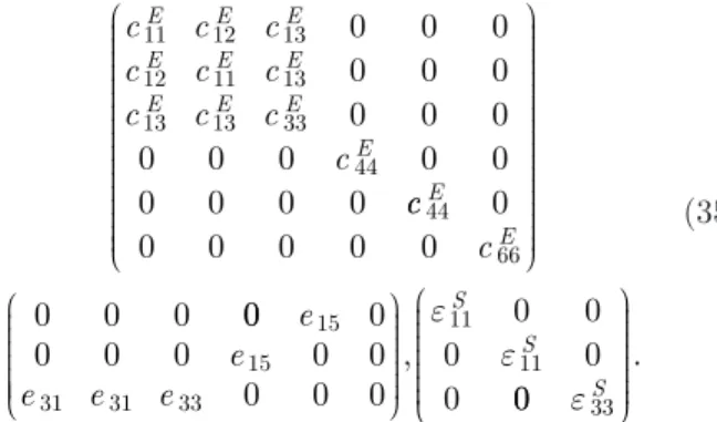
because the axes of poling are different in the primary and secondary sides, the material matrices for each ceram-ic have to be written by respecting the local coordinate system. In this case, for the ceramic poled in the x3 direc-tion, the material matrices of the driving portion take the following expressions [10]: c c c c c c c c c c E E E E E E E E E E 11 12 13 12 11 13 13 13 33 44 0 0 0 0 0 0 0 0 0 0 0 0 0 0 0 0 0 0 cc c E E 44 66 0 0 0 0 0 0 0 0 0 æ è çç çç çç çç çç çç çç ççç ö ø ÷÷÷ ÷÷÷ ÷÷÷ ÷÷÷ ÷÷÷ ÷÷÷ ÷ 00 0 0 0 0 0 0 0 0 0 , 0 0 0 0 0 15 15 31 31 33 11 11 e e e e e S S æ è çç çç ççç ö ø ÷÷÷ ÷÷÷ ÷ e e 00 e33S æ è çç çç ççç ö ø ÷÷÷ ÷÷÷ ÷÷. (35)
For the ceramic poled in the x1 direction, which is used to
define the receiving section, the material matrices can be obtained from the previous matrices by rotating rows and columns properly. They are expressed as
c c c c c c c c c c D D D D D D D D D D 33 13 13 13 11 12 13 12 11 66 0 0 0 0 0 0 0 0 0 0 0 0 0 0 0 0 0 0 cc c h D D 44 44 33 0 0 0 0 0 0 æ è çç çç çç çç çç çç çç ççç ö ø ÷÷÷ ÷÷÷ ÷÷÷ ÷÷÷ ÷÷÷ ÷÷÷ ÷ hh h h h S S 31 31 15 15 33 11 0 0 0 0 0 0 0 0 0 0 0 0 0 , 0 0 0 0 0 æ è çç çç ççç ö ø ÷÷÷ ÷÷÷ ÷ b b 00 b11S æ è çç çç ççç ö ø ÷÷÷ ÷÷÷ ÷÷. (36)
From these assumptions and geometrical considerations, the constitutive relations of the primary and secondary portions can be simplified. Indeed, after assumption 3 is made, the PT is assumed to undergo an uniaxial stress along the axis x1 and to be free of shear stresses. Thus, the stress and strain vectors are reduced to one component:
{ } = 0 0 0 0 0 { } = 0 0 0 0 0 1 1 T T S S T T é ëê ùûú é ëê ùûú . (37)
moreover, as each layer is assumed to be supplied by a sinusoidal voltage, the electrical field is oriented parallel to the axis (3), in the same direction of the depolarizing field. both electrical field and electrical displacement are consequently reduced to one component:
{ } = 0 0 { } = 0 0 3 3 D D E E T T é ëê ùûú é ëê ùûú . (38)
This leads to the following reduced constitutive relation-ships of the primary part given by
T S E D S E c e e 1 11 1 31 3 3 31 1 33 3 = = -+ e . (39)
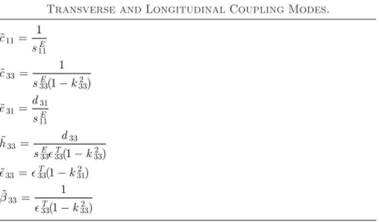
The tilde symbol on the coefficients of the piezoelectric material is a note to use the specific values of the trans-verse coupling mode. These coefficients are given in Table I, where k31 is the material coupling factor relative to the transverse mode.
Furthermore, assuming that the electrical field is con-stant as well as the thickness, the operator matrix Lin can be simply defined by L m t in = -é ë ê ê ù û ú ú, (40)
and as each layer is supplied by the applied voltage Vin(t),
the primary electrical field is defined as
{ } =E N V tin in( ) with Nin = 0 0éëê -m t/ ùûú .T (41)
concerning the receiving section, the insulating and with-out free charges ceramic assures that the components of
electrical displacement along the axes (2) and (3) are equal to zero and, according to Gauss’s law, the component D1 is constant. both electrical field and electrical displacement are consequently reduced to one element:
{ } = 0 0 { } = 0 0 1 1 D D E E T T é ëê ùûú é ëê ùûú . (42)
This leads to the following reduced constitutive relation-ships of the secondary part:
T S D E S D c h h 1 33 1 33 1 1 33 1 33 1 = = - - + b . (43)
The tilde symbol on the coefficients of the piezoelectric material is a note to use the specific values of the longitu-dinal coupling mode. These coefficients are given in Table I, where k33 is the material coupling factor relative to the
longitudinal mode.
In a similar way, the operator matrix Lout can be
sim-ply defined L L out = 1 2 -é ë ê ê ù û ú ú, (44)
and as the piezoelectric transformer produces an output voltage Vout(t), the secondary electrical field is defined as follows:
{ } =E N V ( )t N = 1 L2 0 0
T
out out with out éëê-/ ùûú . (45)
2) Vibratory Analysis: To apply the previously detailed
electromechanical modeling to extract a multimodal mod-el, a preliminary vibratory analysis is necessary to charac-terize the displacement field of extensional modes.
The vibratory study follows the 1-d model of a bar in extension explained in [10]. Furthermore, the number of considered longitudinal modes will be limited to minimize the influence of transverse modes (assumption 2).
accord-TablE I. Piezoelectric material coefficients of the Transverse and longitudinal coupling modes. c sE 11 11 1 = c sE k 33 33 332 1 1 = -( ) e d sE 31 31 11 = h d sE T k 33 33 33 331 332 = - ( ) 33=33T(1-k312) b33 33 332 1 1 = -T( k )
ing to assumption 5, the rosen PT is the association of a primary and secondary parts considered as continuous beams of length L1 (resp. L2), density ρ, and stiffness c11
(resp. c33). From (27) and the reduced constitutive
equa-tions (39) and (43), the following dynamic equilibrium equation in the assumption of linear piezoelectricity is ob-tained: ¶ ¶ ¶ ¶ -¶ ¶ ¶ ¶ 2 1 12 11 2 1 2 1 1 2 1 12 33 2 1 2 = < < 0 = u x u t L x u x u t c c r r for forr 0 <x1<L .2 (46)
according to the free vibrations assumption (assumption 4), the driving and receiving electrodes are considered as short and open, respectively. This means that the driv-ing voltage Vin(t) is equal to zero. Hence, from (43), the expression of the electrical potential along the structure can be obtained: f( ) 1 1 1 33 1 1 1 1 2 ( , ) = 0 < < 0 ( , ) ( ) ( ) 0 < < n x t L x u x t A t x B t x L h , , -+ + ì í ïï î ïïï (47) and A(t) and B(t) are 2 integration constants which may still be functions of time. Physically, A(t) represents the output electric charge and as a consequence the current on the receiving electrode at x1 = L2 [10]. Thus, as the latter is supposed to be open for free vibrations study, A(t) is considered to be equal to zero for vibratory analysis.
concerning the interface conditions, the displacement, the stress, and the electrical potential verify the following continuity relations at the junction of both sections, x1 = 0: u x t u x t T x t T x t x t 1 1 1 1 1 1 1 1 1 ( = 0 , ) = ( = 0 , ) ( = 0 , ) = ( = 0 , ) ( = 0 , ) = - + - + -f f((x1= 0 , )+t. (48)
Furthermore the free-free ends boundary conditions (as-sumption 4) can be written as follows:
T x L t u x x L t T x L t u x c c 1 1 1 11 1 1 1 1 1 1 2 33 1 1 ( = , ) = ( = , ) = 0 ( = , ) = ( - ¶ ¶ -¶ ¶ xx1 =L t2, ) = 0. (49)
To analyze the free vibrations, the harmonic motion as-sumption u1(x1, t) = U(n)(x1)cos(ωt) is considered. Thus,
(46) is modified into d U dx k U L x d U dx k U n n n n n n 2 ( ) 12 1 ( ) ( ) 1 1 2 ( ) 12 2 ( ) ( ) = 0 < < 0 = 0 + -+ for ffor 0 <x1 <L ,2 (50)
which admits the general solution (i = 1, 2)
U n x A k x B k x
i in i in
( )
1 ( ) 1 ( ) 1
( ) = cos( )+ sin( ), (51) where k1( )n and k2( )n are the wave vectors of the nth mode
in the primary and secondary parts, respectively, with the following expressions k s k s k c c n n n E n n n E 1( ) ( ) 11 ( ) 11 2( ) ( ) 33 ( ) 33 33 2 = = = = (1 ) w r w r w r w r - ,, (52)
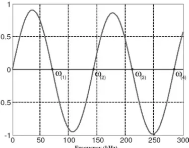
and finally ω(n) is the nth root of the frequency equation given by (a1) and obtained by the determination of con-stants Ai and Bi. a graphic solution of the frequency equa-tion is presented in Fig. 2. The general soluequa-tion of the proposed eigenvalue problem consequently takes the form of (a2). Therefore, in the interests of an appropriate choice of generalized coordinate, the eigenfunction U(n) must be
normalized to match the mechanical generalized coordi-nate with the maximum amplitude of the displacement. The selected criterion of normalization affects the modal mass according to (33). The constant U0( )n consequently
takes the form given by (a3) where the symbol sinc repre-sents the unnormalized sinc function. note that U0( )n is inversely proportional to the square root of a mass and in this instance, if the multiplying constant M0, where M0
is given by (53), is added to normalize the eigenfunction
U(n), the mechanical generalized coordinate will be the
maximum amplitude of the displacement.
M0 =12rwtL (53)
Thus, for applied frequencies close to mechanical resonant frequency, the displacement field of the rosen-type piezo-electric transformer can be finally defined by:
u x t U n x n t
1( , ) =1 ˆ( )( )1hw( )( ), (54)
where hw( )n and Uˆ( )n are, respectively, the mechanical
gen-eralized coordinates representing the maximum amplitude of the displacement and the normalized eigenfunction of the nth extensional mode with:
ˆ .
U( )n x M U n x
1 0 ( ) 1
( ) = ( ) (55)
as the consequence, the assumed mechanical mode shape matrix λm can be defined as
lm n U x U x = ( ) ( ) 0 0 0 0 (1) 1 ( ) 1 ˆ ˆ . æ è çç çç ççç ö ø ÷÷÷ ÷÷÷ ÷ (56)
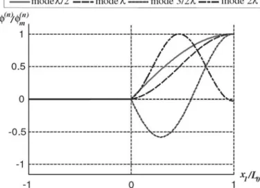
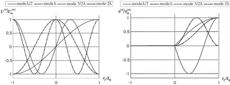
The normalized mechanical displacement of the first 4 lon-gitudinal modes for a rosen PT with equal primary and secondary lengths are shown in Fig. 3; λ represents the wavelength of the vibratory phenomenon. note that the location of the nodal point is sensitive to the difference of stiffness between the driving and receiving parts. In fact, in the case that compliances of both sections verify the inequality sE sE k
11< 33(1- 332), the nodal point of the first
extensional mode appears in the left half where the mate-rial is more rigid in the x1 direction. In Fig. 4, the
normal-ized electrical potential of the first 4 extensional modes functions of x1 are represented. ϕ(1) and ϕ(2) rise in
receiv-ing part. That is why rosen-type PT are generally de-signed to operate at the first 2 extensional modes [9].
3) Application of Hamilton’s Principle: after the
vi-bratory analysis is made, the Hamilton’s principle is ap-plied. according to the general analytical formulation, the lagrangian of the rosen PT can be expressed by (23). by calculating the integral in (24) and using the criterion of normalization (33), the modal mass matrix of the rosen PT is diagonal and reads
M M M n
[ ]
æ è çç çç çç çç çç ö ø ÷÷÷ ÷÷÷ ÷÷÷ ÷÷ = 0 0 0 0 0 0 (1) ( ) , (57)where the modal mass of the ith mode is equal to M0. The total stiffness matrix can be calculated from (19) and (24). by using the equation of normalization (34), the diagonal-ization of the stiffness matrix is achieved as follows:
K K K n
[ ]
æ è çç çç çç çç çç ö ø ÷÷÷ ÷÷÷ ÷÷÷ ÷÷ = 0 0 0 0 0 0 (1) ( ) , (58)where the modal stiffness of the ith mode is given by (59), where the piezoelectric material coefficient of the trans-verse and longitudinal coupling modes (Table I) have been used. K U wt L s k L k L k i i E i i i ( ) 0( ) 2 1 11 1 ( ) 1 2 1 ( ) 1 2 1( = ( ) 2 ( ) 1 (2 ) ( ˆ cos - sinc )) 1 2 33 332 2 ( ) 2 2 2 ( ) 2 2 ) 2 (1 )( ) 1 (2 ) L wt L s k k L k L E i i é ë ê ê + --sinc cos ((k L2( )i 2) ù û ú ú (59)
The electromechanical coupling matrices of the driving and receiving sections take the form of a column vector as follows: y y y y y y in in in out out out
[
]
æ è çç çç çç ç ö ø ÷÷÷ ÷÷÷ ÷÷[
]
= = (1) ( ) (1) n , (( )n æ è çç çç çç ç ö ø ÷÷÷ ÷÷÷ ÷÷, (60)where the modal electromechanical factor of the ith mode of the primary and secondary portions are given by
y y in out ( ) 0 ( ) 31 11 1( ) 1 1( ) 1 = 1 ( ) ( ) i i E i i U mwd s k L k L é ëê ùûú ˆ -coscos (( ) 0 ( ) 2 33 33 2 ( ) 2 2( ) 2 = 1 ( ) ( ) i i E i i U wt L d s k L k L é ëê ùûú ˆ -coscos . (61)
The input and output “blocked” capacitances of the rosen PT can be simply defined by a scalar as
C C m wL k e C C wt k L T T in in out out
[
]
-[
]
-= = (1 ) = = (1 ) 2 1 33 312 33 332 2 e e . (62)by applying Hamilton’s principle, the dynamic equilib-rium of a rosen PT is governed by one matrix equation and 2 scalar relations:
M K V V C V q T
[ ]
+-[
]
+ { } [ ]{ } = [ ] [ ] { } = h h y y y h y in in out out in in in inoutt out out out
[
]
+ ì í ïï ïïï î ïï ïïï T C V q { } =h . (63)The second-order mechanical equation shows a resonant phenomenon whose characteristic modal frequency fr( )i
takes the form
f K M ri i i ( ) ( ) ( ) = 1 2p . (64)
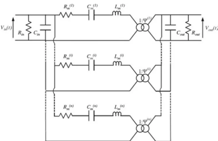
by manipulating (63), the rosen-type PT’s vibratory be-havior can be represented by an equivalent circuit (Fig. 5) where resistances have been added to take into account the dielectric and mechanical losses. The modal mechani-cal losses are represented by a resistance Rm( )i which is
in-versely proportional to the mechanical quality factor Qm of piezoelectric material.
The dielectric losses at the primary and secondary sec-tions are respectively symbolized by the resistances Rin and Rout, estimated by the dielectric loss angle. The
mod-al transformer ratio of the rosen PT is mod-also introduced and is given by y y y ( ) ( ) ( ) = i i i in out . (65)
B. Modeling of Simplified Homogeneous PT
a current simplified analytical model of the electrome-chanical behavior of a rosen-type PT is to consider the structure as a homogeneous medium. In this section, the presented method is newly applied from this additional assumption. as a consequence, the stiffness of the primary side close to the one of the secondary part is implicitly supposed. This assumption takes the following analytical form: c c s s k E E 33 11 11 33 332 = (1- )» .1 (66)
Thus, to determine the electrodynamical characteristics, the application of Hamilton’s principle requires a new vi-bratory analysis to obtain the displacement field. conse-quently, consider the rosen PT as a continuous and ho-mogeneous beam of length L0, density ρ, and stiffness c. newton’s second law applied on a slice of length dx1 gives, in the assumption of linear elasticity,
¶ ¶ ¶ ¶ 2 1 12 2 1 2 = u x c u t r . (67)
Following the example of the previous vibratory analy-sis, by making the free-free ends boundary conditions and harmonic motion assumptions, the solution of free vibra-tions problem can be expressed as follows:
V U k x k L k x k n n n n n n ( ) 0( ) ( ) 1 ( ) 1 ( ) 1 0( ) ( = [ ( ) ( ) ( )] [ (
cos tan sin cos -f nn)x k Ln k xn 1)- -1 ( ( ) 1) ( ( ) 1)] é ë ê êê ù û ú úú tan sin , (68) where k(n) is the wave vectors of the nth mode in the rosen
PT. contrary to the previous study, the wave vector has an analytical expression which is obtained by calculating the constants of integration:
k n L n ( ) 0 = p. (69)
Therefore, to match the mechanical generalized coordi-nate to the maximum amplitude of the displacement, the normalization of the displacement field can be made just by substituting k1( )n and k2( )n by k(n) in the expression of
the constant U0( )n. The same will be true of the calculus of
the modal matrices (mass, stiffness, and electromechanical factor) during the application of Hamilton’s principle. The normalized mechanical displacements of the first 4
tudinal modes are shown in Fig. 6 for a rosen PT with equal primary and secondary lengths. It can be noted that, contrary to the previous vibratory analysis, the as-sumed homogeneity along the x1 direction makes normal-ized mechanical displacement of extensional modes cen-tered in the middle of the structure. In Fig. 7, the normalized electrical potential of the first 4 modes func-tions of x1 are represented.
Hereafter, comparison between the electrodynamical and electrical characteristics of both analytical models will be detailed.
C. Comparisons of Both Models
To check the relevance of both electromechanical mod-els, a noliac ceramic multilayer Transformer (cmT; no-liac Group, Kvistgaard, denmark) is considered [11]. The piezoelectric material used in PT’s processing is a lead zirconate titanate ceramic. The geometric parameters and the material properties are itemized in Table II.
according to Table II, modal electromechanical param-eters of nonhomogeneous PT model can be calculated from (57)–(62). They are shown in Table III. For the ho-mogeneous model, the modal characteristic parameters are obtained by simply substituting k1( )n and k2( )n by k(n) in
(57)–(62). These parameters are detailed in Table Iv. In Tables III and Iv, the series resonant frequencies at short and open receiving electrode are added. Their expressions take the form
f K M f K M KC s =21 p =21 1 2 p p y , æèççç + out öø÷÷÷÷. out (70)
comparisons of results in Tables III and Iv lead to several conclusions about accuracy and interest of these models. First, the vibratory behavior defined by the reso-nant frequencies, modal stiffness, and modal mass is quite similar in both cases. according to mass normalization assumption, both models modal mass is constant regard-less of the vibratory mode. second, significant differences
Fig. 6. normalized mechanical shape of the first 4 modes. Fig. 7. normalized electrical potential of the first 4 modes.
TablE II. noliac ceramic multilayer Transformer rosen Piezoelectric Transformer’s Geometric Parameters and material Properties.
definition value Unity
L1 Primary length 12 mm L2 secondary length 13 mm w Width 5 mm t Thickness 1.7 mm m Primary layers 16 ρ mass density 7600 kg/m3 sE
11 Transversal compliance at constant E 1.256e−11 m2/n
sE
33 longitudinal compliance at constant E 1.610e−11 m2/n
d31 Transversal piezoelectric coefficient −1.329e−10 m/n d33 longitudinal piezoelectric coefficient 3.086e−10 m/n
33T Permittivity at constant T 14540 F/m
k31 Transversal coupling factor 0.330
k33 longitudinal coupling factor 0.678
Qm mechanical quality factor 1000
appear on electromechanical conversion factors except for the (λ)-mode. more generally, modal characteristics of both models are similar for the (λ)-mode. The weak influ-ence of nonhomogeneous media on the even waveforms can give the proof of this noteworthy agreement.
another significant difference is observed on the elec-trical potential repartition along the receiving part, par-ticularly for the (3/2λ)-mode. an obvious difference of the extremum values of the electrical potential appears on Figs. 4 and 7. These curves are obtained from equa-tions (a1) and (68), respectively. This difference lies in the value of k(n) factor and L
1/L2 ratio. The singular unit
waveform on Fig. 7 appears in the case of consideration of homogeneous medium and equal primary and second-ary lengths.
In intermediate conclusion about both models com-parisons, it can be deduced that the choice of analyti-cal approach and assumption considerations depend on the model’s final objective. a simple model will be a sufficient approximation in the case of single mode con-sideration. The most complete model becomes necessary if a multimodal approach is required for optimization problems without arbitrary selected mode or in the case that the electrical potential repartition is a considered point of view.
In following section, previous analytical values will be compared with results obtained by finite elements method and experimental results.
Iv. numerical and Experimental validation To verify the rosen-type PT analytical electrodynami-cal model, a numerielectrodynami-cal study and an experimental identi-fication were undertaken.
The experimental identification of the electrical equiva-lent circuit of the cmT noliac transformer has been led for the first 4 longitudinal vibratory modes and previously undertaken in [12]. This identification is based on admit-tance measurements with agilent HP 4294a impedance analyzer (agilent Technologies Inc., santa clara, ca).
by two successive characterizations with the input and output terminal shorted, respectively, the electrical equiv-alent circuit is fully identified [13].
The following part is dedicated to briefly introduc-ing the numerical method. The aim of this approach is to validate the theoretical modal mechanical shapes and electrical potentials and to extract the electromechanical parameters of the PT.
A. Development of Numerical Method
The method to characterize the double electromechani-cal conversion is based on a modal analysis and energy considerations using a finite element method with the an-sys software. The modal study concerns the longitudinal mode of a PT composed of 2 rectangular piezoelectric ce-ramics of length L1 (resp. L2), width w, thickness t, and
TablE III. modal Parameters of nonhomogeneous rosen-Type Piezoelectric Transformer model.
mode λ/2 mode λ mode 3/2λ mode 2λ
fs [Hz] 63 686 123 430 190 790 247 420 fp [Hz] 69 276 139 630 194 520 247 420 Cin [nF] 103.63 103.63 103.63 103.63 Cout [pF] 4.551 4.551 4.551 4.551 M [g] 0.808 0.808 0.808 0.808 K [Gn/m] 0.129 0.486 1.161 1.952 Lm [mH] 0.823 0.285 1.569 287.9 Cm [nF] 7.584 5.833 0.443 0.001 ψin [c/m] 0.990 1.683 −0.717 −0.053 ψout [c/m] 0.0104 −0.0249 −0.0144 0.0006 ψ 95.37 −67.68 49.70 −96.52
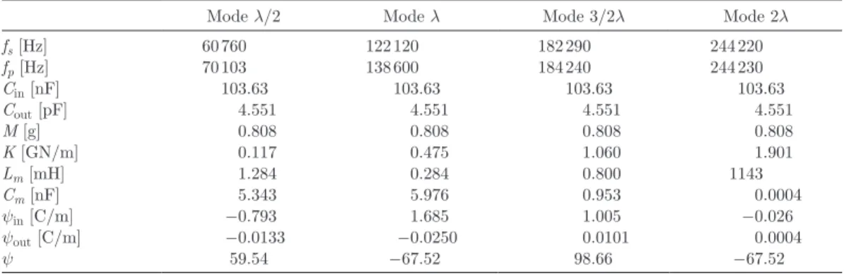
TablE Iv. modal Parameters of Homogeneous rosen-Type Piezoelectric Transformer model.
mode λ/2 mode λ mode 3/2λ mode 2λ
fs [Hz] 60 760 122 120 182 290 244 220 fp [Hz] 70 103 138 600 184 240 244 230 Cin [nF] 103.63 103.63 103.63 103.63 Cout [pF] 4.551 4.551 4.551 4.551 M [g] 0.808 0.808 0.808 0.808 K [Gn/m] 0.117 0.475 1.060 1.901 Lm [mH] 1.284 0.284 0.800 1143 Cm [nF] 5.343 5.976 0.953 0.0004 ψin [c/m] −0.793 1.685 1.005 −0.026 ψout [c/m] −0.0133 −0.0250 0.0101 0.0004 ψ 59.54 −67.52 98.66 −67.52
poled in the x3 (resp. x1) direction (Fig. 8). because of the
thin beam geometry and the range of interest of vibratory modes, the numerical study comes down to extensional modes along the axis x1.
The primary and secondary sides have to be separately created by introducing 2 local coordinate systems to de-fine the material matrices of each piezoelectric ceramic from (35) and (36). after defining the structure, the deter-mination of the electromechanical characteristics requires a modal study. This procedure, in which the primary and secondary sections are short-circuited and open, respec-tively, enables the determination of the modal mass, the modal stiffness, the modal electromechanical conversion factors, and the modal transformer ratio. This method relies on the calculus for each longitudinal mode of the res-onant frequency fp, the maximum amplitude of
displace-ment ηm, the kinetic energy T, the potential energy U, the
charge on the primary electrode qin, and the secondary
electrical potential Vout. by knowing these different
quan-tities, the electromechanical parameters can be obtained by the following equations:
M T f K U mq C V p m m m m = 2 (2 ) = 2 = = 2 2 2 p h h y h y h , , , .
in in out out out
(71)
according to the previous expressions of the electrome-chanical parameters, the electrical characteristics (mo-tional inductance and mo(mo-tional capacitance) can be ex-tracted as follows: L M C K m = 2 m = 2 y y in in , . (72)
a modal study where the driving and receiving sections are short-circuited is also undertaken to extract the series resonant frequency fs. The modal values are itemized in
Table v.
B. Validation of Analytical Models
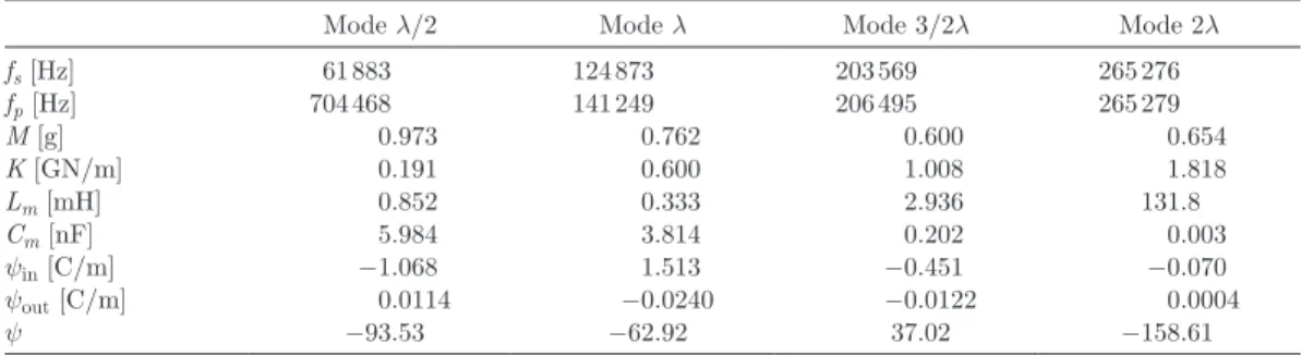
Figs. 9 and 10 show the numerically obtained normal-ized mechanical shape and electrical potential, respective-ly, of the first 4 modes. It appears clear that the curves, as much for the modal mechanical displacements as for the modal electrical potentials, are quite similar with the ones from nonhomogeneous rosen-type PT model. The nodes and antinodes of modal shapes are effectively located in the left half of the structure in conformity with the non-homogeneous model. Furthermore, the vibratory behav-ior defined by the modal parameters is in line with the analytical values for the (λ/2)- and (λ)-modes. The pe-culiar vibratory behavior of the (2λ)-mode, underlined by the theoretical model, is also confirmed by the numerical study. Indeed, the very close values of series resonant fre-quencies fs and fp and the weak electromechanical
conver-sion factors ψin and ψout can testify to this phenomenon.
as the experimental identification is obtained by admit-tance measurement, Fig. 11 shows the input admitadmit-tance simulated by analytical and numerical models and the lat-ter are compared with experimental results. Fig. 12
illus-TablE v. modal Parameters of numerical rosen-Type Piezoelectric Transformer model.
mode λ/2 mode λ mode 3/2λ mode 2λ
fs [Hz] 61 883 124 873 203 569 265 276 fp [Hz] 704 468 141 249 206 495 265 279 M [g] 0.973 0.762 0.600 0.654 K [Gn/m] 0.191 0.600 1.008 1.818 Lm [mH] 0.852 0.333 2.936 131.8 Cm [nF] 5.984 3.814 0.202 0.003 ψin [c/m] −1.068 1.513 −0.451 −0.070 ψout [c/m] 0.0114 −0.0240 −0.0122 0.0004 ψ −93.53 −62.92 37.02 −158.61
Fig. 9. numerical normalized mechanical shape of the first 4 modes. Fig. 8. 3-d deformed structure.
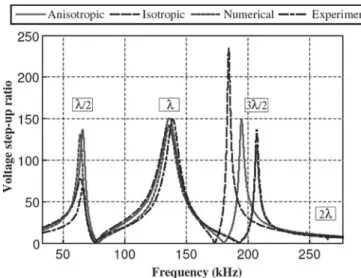
trates the voltage step-up ratio obtained by simulation of the equivalent multimodal electrical circuit (Fig. 5). ac-cording to these both figures, a convenient accuracy for the first 2 (λ/2)- and (λ)-modes can be noted between the different approaches. This comparison proves the validity of the assumption (66) about consideration of homogeneous medium. Then, an obvious divergence between models appears at the third longitudinal vibratory mode. If the nonhomogeneous model may be considered as acceptable, the homogeneous one presents a widely undervalued reso-nant frequency. From this mode, it can be considered the limit of validity of 1-d approximation for these dimensions, whereas the numerical model is still convenient. another comment can be made about the peculiar (2λ)-mode: if the analytical and numerical models shows its existence, the first transverse mode predominates experimentally in the vicinity of the latter and the identification of its modal
characteristics is made impossible. The frequency location of this first transverse mode can be proved by a numerical study and is also confirmed in [14].
Finally, it can be noted that amplitude accuracy of nonhomogeneous and numerical models depends on load choice. Indeed, waveform is affected by the latter, leading to displacement of the nodes and consequently the modal parameters values.
v. conclusion
a general multimodal electromechanical method of a freely vibrating PT based on Hamilton’s principle was presented. The main interest of this analytical approach was to obtain a dimensioning model for inverse problem formulation to deduce the optimal dimensions. moreover, this general method can be applied to several kinds of PT geometry with multiple driving and receiving sec-tions, and also without imposing beforehand a vibratory mode rank. To validate the proposed model, the classic rosen-type PT was considered and the nonhomogeneous and homogeneous PT assumptions are made. The modal characteristics, mechanical shapes, and electrical poten-tials were obtained and compared for both approaches. The analytical models are pertinent and their use depends only on the considered point of interest (for example: elec-trical potential repartition study, single-mode study, etc.). Finally, a comparison between the theoretical, numerical, and experimental results was presented and a good agree-ment was obtained.
appendix a
• Frequency equation of the nonhomogeneous Rosen-type PT model:
Fig. 11. Input admittance modulus of rosen piezoelectric transformer for 500 kΩ load.
Fig. 12. voltage step-up ratio of rosen piezoelectric transformer for 500 kΩ load.
s k s k L k L k L E E n n n 33 332 11 1 ( ) 1 2( ) 2 1( ) 1 (1 ) ( ) ( ) ( ) ( -+ sin cos cos sinkk Ln 2( ) 2) = 0 (a1)
General solution of eigenvalue problem based on the •
nonhomogeneous rosen-type PT model: see (a2), above.
• normalization constant of modal mechanical shapes from the nonhomogeneous rosen-type PT model:
U wt L k L k L L k n n n n 0( ) 1 1 ( ) 1 2 1( ) 1 2 2 ( = 1 1 2 1 (2 ) ( ) 1 (2 r +sinc + +sinc cos )) 2 2 2( ) 2 ) ( ) L k Ln cos é ë ê êê ù û ú úú (a3) references
[1] c. rosen, “ceramic transformers and filters,” in Proc. Electronic
Components Symp., 1956, pp. 205–211.
[2] s.-T. Ho, “design of the longitudinal mode piezoelectric transform-er,” in 7th Int. Conf. Power Electronics and Drive Systems, nov. 2007, pp. 1639–1644.
[3] s.-T. Ho, “modeling and analysis on ring-type piezoelectric trans-former,” IEEE Trans. Ultrason. Ferroelectr. Freq. Control, vol. 54, no. 11, pp. 2376–2384, nov. 2007.
[4] F. Pigache, F. messine, and b. nogarede, “optimal design of piezo-electric transformers: a rational approach based on an analytical model and a deterministic global optimizations,” IEEE Trans.
Ul-trason. Ferroelectr. Freq. Control, vol. 54, no. 7, pp. 1293–1302, July.
2007.
[5] H. Tiersten, “Hamilton’s principle for linear piezoelectric media,” in
Proc. IEEE, vol. 55, no. 8, pp. 1523–1524, aug. 1967.
[6] n.-W. Hagood and a.-J. mcFarland, “modeling of a piezoelectric rotary ultrasonic motor,” IEEE Trans. Ultrason. Ferroelectr. Freq.
Control, vol. 42, no. 42, pp. 210–224, mar. 1995.
[7] m. Geradin and d. rixen, Mechanical Vibrations Theory and
Ap-plications to Structural Dynamics, 2nd ed. new york, ny: Wiley,
1997.
[8] IEEE Standard on Piezoelectricity, ansI/IEEE standard 176-1987, 1988.
[9] E. Horsley, m. Foster, and d. stone, “state-of-the-art piezoelectric transformer technology,” presented at Eur. Conf. Power Electronics
and Applications, 2007.
[10] J. yang and X. Zhang, “Extensional vibration of a nonuniform pi-ezoceramic rod and high voltage generation,” Int. J. Appl.
Electro-magn. Mech., vol. 16, no. 12, pp. 29–42, 2002.
[11] http://www.noliac.com/default.aspx?Id=7781
[12] J. F. lopez, “modeling and optimization of ultrasonic linear mo-tors,” Ph.d. dissertation, Ecole Polytechnique Fédérale de lau-sanne, november 2006.
[13] r.-l. lin, “Piezoelectric transformer characterization and applica-tion of electronic ballast,” Ph.d. dissertaapplica-tion, virginia Polytechnic Institute and state University, nov. 2001.
[14] v. Karlash, “Electroelastic vibrations and transformation ratio of a planar piezoceramic transformer,” J. Sound Vibrat., vol. 277, pp. 353–367, 2004.
Clement Nadal was born in rennes, France, in
1983. He received the dipl. Ing. degree in electri-cal engineering from Ecole nationale supérieure d´Electrotechnique, d´Electronique, d´Informa-tique, d´Hydraulique et des Télécommunications (EnsEEIHT), Toulouse, France, and the m.s. de-gree in electrical engineering from the Institut na-tional Polytechnique de Toulouse in 2007. He is now a Ph.d student in the Electrodynamics GrEm3 research group of the laboratoire des Plasmas et de la conversion d’Energie (laPlacE), Toulouse, France.
Francois Pigache was born in auchel, France, in
1977. He received the m.s. degree in instrumenta-tion and advanced analysis in 2001, and the Ph.d. degree in electrical engineering from the Univer-sity of sciences and Technology of lille, France, in 2005. He joined the laboratoire des Plasmas et de la conversion d’Energie (laPlacE), Tou-louse, France, as an assistant professor where his research concerns the multi-physics modeling and the optimization of piezoelectric transformers.
V x U x U k x k L k x n n n n n n ( ) 1 ( ) 1 0( ) 1 ( ) 1 1( ) 1 1( ) ( ) =
( ) = cos( )-tan( )sin( 11 1 1
2( ) 1 2( ) 2 2( ) 1 1 2
) < < 0 ( ) ( ) ( ) 0 < <
,
cos tan sin ,
-+ ì L x k xn k Ln k xn x L íí ïïï î ïïï -- + f( ) f 1 0( ) 1 1 2( ) 1 2( ) ( ) = 0 < < 0 ( ) 1 ( n n n n x L x k x k L ,
cos tan 22)sin(k x2( )n 1) 0 <, x1<L2
ì í ïï îïï é ë ê ê ê ê ê ê ê ù û ú ú ú ú ú ú ú (a2)