HAL Id: tel-01891046
https://tel.archives-ouvertes.fr/tel-01891046 Submitted on 9 Oct 2018
HAL is a multi-disciplinary open access
archive for the deposit and dissemination of sci-entific research documents, whether they are pub-lished or not. The documents may come from teaching and research institutions in France or abroad, or from public or private research centers.
L’archive ouverte pluridisciplinaire HAL, est destinée au dépôt et à la diffusion de documents scientifiques de niveau recherche, publiés ou non, émanant des établissements d’enseignement et de recherche français ou étrangers, des laboratoires publics ou privés.
networks
Jaafar Bendriss
To cite this version:
Jaafar Bendriss. Cognitive management of SLA in software-based networks. Networking and Internet Architecture [cs.NI]. Institut National des Télécommunications, 2018. English. �NNT : 2018TELE0003�. �tel-01891046�
l’UNIVERSIT ´E PIERRE ET MARIE CURIE Sp´ecialit´e
Informatique et r´eseaux Pr´esent´ee par
Jaafar BENDRISS
Pour obtenir le grade de
DOCTEUR de TELECOM SUDPARIS
Sujet de la th`ese :
Gestion Cognitive de SLA dans un contexte NFV
soutenue le 14 juin 2018 devant le jury compos´e de :
Prof. Djamal Zeghlache Directeur de th`ese Telecom SudParis Dr. Imen Grida Ben Yahia Encadrante de th`ese Orange Labs
Prof. Panagiotis Demestichas Rapporteur University of Piraeus
Prof. Filip de Turck Rapporteur Ghent University
Prof. Marcelo Dias de Amorim Examinateur LIP6
Mdme Marie-Paul Odini Examinatrice HP
1 Introduction 1
I Introduction . . . 1
II Problem Statement . . . 3
A Research Questions . . . 4
B Contributions . . . 5
III Thesis Structure . . . 6
2 Machine Learning : Basics, Challenges, and Network Applica-tions 9 I Introduction to Machine Learning (ML) . . . 10
A Definition . . . 10
B Machine Learning Types . . . 13
C A Brief History of Machine Learning . . . 14
II Supervised Machine Learning . . . 16
A How machines learn. . . 24
B Evaluation . . . 33
III Unsupervised Machine Learning . . . 41
A Clustering . . . 41
B Anomaly Detection . . . 42
C Dimetionality Reduction . . . 42
IV Deep Learning . . . 44
A How Deep Learning is different? . . . 45
B Exploding/Vanishing gradients problem . . . 45
C Regularization . . . 47
D RNN . . . 47
V Machine Learning Latest Challenges . . . 49
A Machine vs Human Learning . . . 49
B Scalable Machine Learning . . . 50
VI Machine Learning for Network Management . . . 53
A Machine Learning for Network Management a Brief History . . . 55
B FCAPS Management . . . 57
C Cognitive Network Management Initiatives . . . . 60
VII Conclusion . . . 66
3 SLA management 67 I Context : Software Networks . . . 68
A Network Function Virtualization . . . 68
B Software-Defined Networking . . . 70
II Early SLA management . . . 73
III SLA in the Cloud . . . 74
IV SLA in Software Networks . . . 77
V Literature Gaps and Future Research Directions . . . 80
4 Proposal : Cognitive SLA Management Framework 83 I Introduction . . . 84
II Problem Statement . . . 87
A Service Level Agreement . . . 89
B SLA and SDN/NFV . . . 90
C Formal Description . . . 92
D SLA Example . . . 93
III Cognitive SLA Architecture . . . 95
A Cognet Smart Engine : . . . 98
B Policy Engine . . . 101
C NFV Architectural Framework . . . 102
D Proposed workflow . . . 103
E Policy Engine . . . 107
F Cognet Sequence Diagram . . . 108
G Operational Application & Use Cases . . . 109
IV Data Analysis . . . 124
A Data Gathering . . . 124
B Data preparation . . . 126
C Dimensionality reduction . . . 129
D Visualization . . . 138
5 Proposal : Cognitive Smart Engine 145
I Introduction . . . 146
II CSE Algorithms . . . 149
A Anticipation and forecasting . . . 150
B Classification . . . 157
III Model selection . . . 171
A Problem Formulation and Choices . . . 171
B Search Methods . . . 173
C The hyperparameter Search Space . . . 177
D Research Methodology . . . 182 E Data . . . 183 F Meta-Learning . . . 188 G feature relevance . . . 193 IV Conclusion . . . 195 A Thesis Publications 197 I List of Contributions . . . 197 A Accepted papers . . . 197
B Public Cognet Deliverables . . . 198
C Exhibition . . . 199
1.1 The cost of hardware and software and their management
[1]. . . 4
1.2 Research question mindmap. . . 6
1.3 Thesis structure . . . 8
2.1 Machine Learning approach . . . 11
2.2 Machine Learning vs programming . . . 12
2.3 Machine Learning can provide deeper understanding of old problems . . . 12
2.4 Machine Learning types and different tasks type . . . 13
2.5 Randomy generated data. the x-axis represent the input and y-axis represents the target values. . . 18
2.6 Machine Learning types and different tasks type . . . 18
2.7 a Biological neuron [2] . . . 19
2.8 Artificial perceptron and its decision boundary . . . 19
2.9 Non-linear decision boundary XOR . . . 21
2.10 MLP solving XOR problem . . . 21
2.11 MLP solving XOR problem . . . 21
2.12 simple MLP example . . . 22
2.13 Gradient Descent . . . 25
2.14 Gradient Descent with a learning rate too small and too large . . . 27
2.15 Optimizer comparison . . . 28
2.16 Activation functions and their respective derivatives . . . 31
2.17 bias vs variance . . . 34
2.18 Classification metrics. Precision and recall . . . 36
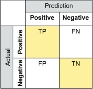
2.19 Confusion matrix . . . 37
2.20 bias vs variance . . . 40
2.21 Machine Learning Diagnostic process . . . 40
2.22 Clustering example . . . 42
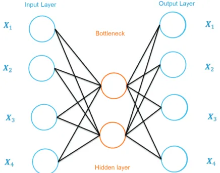
2.23 Shemetic structure of an autoencoder with one fully connec-ted hidden layer. . . 43
2.24 Saturation . . . 46
2.25 RELU activation function . . . 46
2.26 LSTM Cell : The element wise multiplication is key for LSTM cell, helping the preservation of constant error when backpropagating the error. The forget gate is an identity function, when it is open the input is multiplied by 1. . . 48
2.27 The process of ML research . . . 52
2.28 The evolution of machine learning and Network Manage-ment . . . 56
2.29 IBM’s MAPE-K (Monitor, Analyze, Plan, Execute, Know-ledge) reference model for autonomic control loops . . . . 61
3.1 NFV reference architecture . . . 69
3.2 SDN Architecture . . . 72
3.3 Overall feedback on the importance of the ”Proactive SLA violation detection” research area [3]. . . 77
4.1 PhD Blueprint. . . 87
4.2 Simplified UML diagram of SLA. . . 90
4.3 SLA NFV description In ETSI framework . . . 91
4.4 SLO step function of response time. . . 94
4.5 Cognet architecture . . . 97
4.6 Cognet Smart Engine . . . 99
4.7 Data Pre-processing . . . 103
4.8 Processing Engines. . . 105
4.9 Processing Engines. . . 107
4.10 Cognet global architecture sequence diagram. . . 109
4.11 Simplified Cognitive SLA Architecture. . . 110
4.12 UML and data model for CogSLA. . . 111
4.13 Overview of Prometheus data set. . . 115
4.14 Overview of Prometheus data set. . . 116
4.15 Network diagram for the streaming use case. . . 118
4.17 Our Testbed. Clearwater virtual IMS functional architec-ture in the box lower right. Upper left the Cognitive Smart Engine (CSE). The experimental process is : (1) Stress tes-ting for SLA violation generation. (2) System-level super-vision. (3) Reporting SLO violations. (4) Data labeling, merging observations on the SLO state and the
system-level metrics. . . 120
4.18 A subset of the data set distribution. The small boxes re-present the quartiles of the distribution. The red line in the middle represents the median, i.e. the point separa-ting the data into half. The outliers are drawn as black crosses outside the box. . . 121
4.19 Cognitive SLA Architecture. . . 122
4.20 CSE implementation choices. . . 123
4.21 Raw data in JSON into a Table . . . 127
4.22 Example of the autocorrelation function applied on the load of the SIP proxy. . . 133
4.23 Lagged autocorrelation. . . 134
4.24 Transforming raw timeseries into stationary ones . . . 134
4.25 Inta VM correlations . . . 135
4.26 Correlation bewteen all the 156 metrics of the testbed. . . 136
4.27 Example of correlation versus causation. . . 138
4.28 time series visualization. . . 139
4.29 T-SNE plot of SLA and SLA Violation. . . 140
4.30 SLO visualized as a radar map. . . 141
4.31 Service Quality Monitor. . . 142
5.1 Zoom on the Main building blocks of the CSE. . . 146
5.2 Picture of a boxplot. . . 148
5.3 Media SLA sequence diagram, focusing on the ML process. 150 5.4 FFNN architecture used for forecasting on 4 features fol-lowing equation 5.1. . . 154
5.5 Normal inputs vector vs recurrent neural network inputs. 155 5.6 Stacked Stateful LSTMs Trained for prediction . . . 156
5.7 Stacked FFNN for predicting . . . 156
5.8 Difference between FFNN and LSTM for signal prediction. 156 5.9 SLO1 targeting the Sprout VNFC. . . 159
5.10 Layout of the dataset used in Use case II. . . 159 5.11 The activation function g(x) - if non-linear - applied to
the output of the neuron allows the ANN to behave as a
universal approximator by introducing non-linearity. . . 161 5.12 Combined FFNN with Decision Tree (MLP-DT) . . . 162 5.13 A miniature representation of our experiments, where
in-puts are limited to 4 (we use 156) and output to one (we used 3). a) is the features represented as time series data. b) is the point of contact, the inputs fed to the ANN mo-del. c) The ANN model which can be LSTM or FFNN. d) is the binary result that categories the inputs into 0 or 1
for non SLA violation and SLA violation respectivelly. . . 163 5.14 Accuracy over all the training steps . . . 165 5.15 Precision over all the training steps . . . 165 5.16 Recall over all the training steps . . . 165 5.17 Precision, recall and accuracy over all the training steps . 165 5.18 Confusion matrix of the Best algorithm (LSTM2) . . . 166 5.19 Results of offline evaluation mode of the FFNN with three
different SLO breach threshold (Based on the streaming
use case) . . . 167 5.20 Example of a subgraph in a Decision Tree over 10.000
sample. . . 169 5.21 Results comparing FFNN and LSTM based on the
valida-tion and test set. . . 170 5.22 The Training time of the FFNN for 10,000 samples. . . 170 5.23 Overall performance of FFNNs vs LSTMs (The model code
are in the index section B) . . . 170 5.24 Methodology. . . 173 5.25 Random search is computationally less expensive and scans
a wider area in the configuration space shown as intercon-nection of gray lines. On the other hand, Random Search is very effective especially when the intuition of the ope-rator fails to approximate the range of the search as shown
in the intersection of red rectangles. . . 177 5.27 Overview of the dynamic ANNs architectures. LSTM on
that dropout regularisation slightly improves the accu-racy with no compromise in time (as represented by
fi-gure 5.29) . . . 188 5.29 Time versus dropout . . . 188 5.30 Accuracy with respect to Activation functions in the
out-put layer. This figure shows that the choice of the
activa-tion layer is amogst the most important ones. . . 188 5.31 Optimizer type with their respective learning rate
ver-sus accuracy. The best optimizer is Adadelta, the worst is
RMSprop. . . 188 5.32 comparison between LSTM and FFNN by accuracy over
the validation set. . . 189 5.33 ANN initialization method versus accuracy. GN : Glorot
Normal, GU : Glorot Uniform, HN : He Normal, HU : He Uniform, LU : Lecun Uniform, N : Normal, O :
Orthogo-nal, U : Uniform, Z : zero. . . 189 5.34 Top 5 best ANNs based on the mean over Globalmetric . . 189 5.35 Top 5 ANNs based on the mean over validation score
ac-curacy. All the best ANNs appear to converge on 94%
ave-rage accuracy. . . 189 5.36 Results for medium ANNs structure (under 30 hidden
layers and 20 average neuron per layer). Point A1 is the global maximum. Point A2 is a local maximum. Point A3 is a local minimum. In the text below, we provide an
in-terpretaion of these results. . . 192 5.37 Feature importance of the table 5.12. . . 195 5.38 Feature importance of the ANNs’ hyperparameters . . . . 195
Acknowledgements
By completing this PhD thesis, I achieved my greatest and long aspi-red goal in my career. It has been with no doubt the happiest and richest experience of my life. The PhD experience enlightened me both perso-nally and professioperso-nally. I have lived this experience with passion.
A special thanks to my PhD supervisor Imen Grida Ben Yahia who trusted me to carry out this project and made hereself always available for guidance and support. It has been a pleasure and a honor to me to work with her. I’ve learned so much I am aware of her print on my work and fr this I am grateful.
I would like also to thank my academic supervisor Djamal Zeghlache who contributed to the elaboration of this thesis and provided me with his precious advice and guidance.
A special thanks to Professor Panagiotis Demestichas and Professor Philip De Turck who evaluated and reviewed my manuscript. I am gra-teful to all my co-workers at Orange Labs who helped me to integrate the team and made this experience memorable. This project would not have been possible without a three year scholarship support from Orange Labs.
Last but not least, I would like to thank my family members who sup-ported me throughout this endeavor. I would like to thank my mother Jamila Touati my Father Aziz Bendriss my aunts Saida and Joudia Touati and my sisters Yasmine and Yousra to whom I feel deeply indebted.
Chatillon, 2018
Table1 – Abbreviation table of common used acronyms. SLA Concepts
SLA Service Level Agreement.
SLO Service Level Objective.
SLOV Service Level Objective Violation.
SLAV Service Level Agreement Violation.
Networking Concepts
SDN Software Defined Infrastructure.
NFV Network Function Virtualization.
NFVI Network Function Virtualization Infrastructure.
VIM Virtual Infrastructure Manager.
VNF Virtual Network Function.
VNFC Virtual Network Function Component.
VNFM Virtual Network Function Management.
VNG-FG Virtual Network Function Forwarding Graph.
ETSI European Telecommunications Standards Institute .
Machine Learning Concepts
DT Decision Tree.
MCDT Multi-Class Decision Tree.
PCA Principal Component Analysis.
RMSE Root Mean Squared Error.
KPI Key Performance Indicator.
ML Machine Learning.
RL Reinforcement Learning.
VM Virtual Machine.
ANN Artificial Neural Network.
FFNN FeedForwad Neural Network.
SVM Support Vector Machine.
RNN Recurrent Neural Network.
LSTM Long Short Term Memory.
RBM Restricted Boltzmann Machine.
ETL Extract Transfer Load.
GPU Graphical Processing Unit.
Other Concepts
CAPEX CAPital EXpenditure .
This thesis addresses cognitive management aspects of Service Level Agreement (SLA) in software-based networks.
Telecommunications operators pushed towards virtualization of their networking function by introducing in 2012 the concept of Network Function Virtualization (NFV). NFV aims at reducing vendor lock-in and bringing agility in the services and resources life cycle operation and management. The IT and networking industries foresee a combined use of SDN and NFV to make cloud and network services agile. Major service and network providers predict that, by 2020, 70% of deployed networks will rely on cloud infrastructures, virtual network functions and multi-domain SDN controllers. This evolution and new require-ments call for efficient SLA enforcement and management. This thesis tackles the following concerns : (1) a formal definition of SLA, (2) proac-tive SLA violation detection methodology and (3) the definition of an ex-tended framework for cognitive management in softwarized networks.
This doctoral work led to an end-to-end data-driven framework, na-mely, CogSLA, which stands for Cognitive SLA. The framework is based on the use of multiple Machine Learning (ML) algorithms in conjunc-tion for improving predicconjunc-tion and anticipaconjunc-tion of SLA violaconjunc-tions. The proposed framework is based on two types of Artificial Neural Net-works (ANNs), The FeedForward Neural NetNet-works (FFNNs) which sho-wed state-of-the-art results in image classification. And a special type of Recurrent Neural Networks with best performance for Natural Lan-guage Processing, the LSTM. Both algorithms have specific advantages and drawbacks, the work was nevertheless able to leverage these algo-rithms for anticipating SLA violations.
The thesis proposes also a meta-algorithm to optimize the tunings of the Artificial Neural Networks (ANN) algorithms in an acceptable time and performance. The proposed approach relies on biased random selection and the use of meta-knowledge obtained from training the first round of ML algorithms on our data set.
A new metric based on information theory and on entropy is also used to classify and assess the relevance of each Machine Learning parameter with respect to performance and accuracy.
R´esum´e
Cette th`ese traite les aspects de la gestion cognitive du niveau de ser-vice (SLA) dans les r´eseaux virtuels. Les op´erateurs de t´el´ecommunications ont pouss´e vers la virtualisation de leurs fonctions r´eseaux en introdui-sant en 2012 le concept de virtualisation de fonction de r´eseau (NFV). NFV vise `a r´eduire le couplage des op´erateurs au profit des construc-teurs r´eseaux et `a apporter plus l’agilit´e dans l’exploitation et la gestion du cycle de vie des services et des ressources. Les secteurs de l’infor-matique et des r´eseaux pr´evoient une utilisation combin´ee du SDN et du NFV pour rendre les services de Cloud et de r´eseau plus agiles. Les principaux fournisseurs de services et de r´eseaux pr´evoient que d’ici 2020, 70% des r´eseaux d´eploy´es d´ependront des infrastructures Cloud, des fonctions virtualis´ees et des contrˆoleurs SDN multi-domaine. Cette ´evolution exige une application et une gestion efficaces des SLA. Cette th`ese vise `a r´epondre `a trois points essentiels : (1) une d´efinition for-melle du SLA dans les r´eseaux virtualis´es, (2) une m´ethodologie proac-tive de d´etection des violations de SLA et (3) la d´efinition d’un Frame-work pour la gestion cognitive dans les r´eseaux logiciels.
Premi`erement, nous avons propos´e un Framework ax´e sur les donn´ees de bout en bout, `a savoir CogSLA. Le cadre est bas´e sur l’utilisation de plusieurs algorithmes de Machine Learning (ML) en conjonction pour am´eliorer la pr´ediction et l’anticipation des violations de SLA. Le Fra-mework propos´e est bas´e sur deux types de r´eseaux neuronaux (ANN), les r´eseaux neuronaux de type FeedForward (FFNN) qui ont montr´e des r´esultats satisfaisant dans la classification des images. Et un type parti-culier de r´eseaux neuronaux r´ecurrents (RNN) disposant des meilleures performances pour le traitement du langage naturel, le LSTM. Les r´esultats montrent que les deux algorithmes ont des avantages et des inconv´enients sp´ecifiques, mais nous d´emontrons qu’ils peuvent ˆetre utilis´es de mani`ere diff´erente pour anticiper les violations de SLA.
Deuxi`emement, nous avons propos´e un m´eta-algorithme pour opti-miser les ajustements des r´eseaux de neurones artificiels (ANN) avec un temps d’apprentissage et une performance acceptable. L’approche pro-pos´ee repose sur la s´election al´eatoire biais´ee et l’utilisation de m´eta-connaissances obtenues `a partir de la formation du premier tour de
Al-Enfin, nous proposons une nouvelle m´etrique bas´ee sur la th´eorie de l’information et sur l’entropie pour classifier et ´evaluer la pertinence de chaque param`etre de Machine Learning en termes de performance et de pr´ecision.
Introduction
The greatest enemy of knowledge is not ignorance, it is the illusion of knowledge.
Stephen Hawking.
I
Introduction
The softwarization of networks is a reality today. The emergence of Network Function Virtualization (NFV) and Software Defined Networ-king (SDN) are expected to bridge the gap between the Telco and IT industries. NFV allows the virtualization of network function by de-coupling the software and hardware. A network function can be intru-sion detection system, firewall and signaling systems. This allows more flexibility, reduces Time-To-Market TTM and free the Telco from vendor lock-in. The network function can run on commodity hardware such as x86 servers. Consequently, the Telco are expecting to reduce their CA-PEX and OCA-PEX. SDN builds programmable networks through abstrac-tions, open APIs (northbound and southbound) and the separation of control and data planes. NFV targets the virtualization of network func-tions and aims at reducing vendor lock-in and bringing agility in the services and resources lifecycle operation and management. The IT and networking industries foresee a combined use of SDN and NFV to make cloud and network services agile. Major service and network providers
predict that, by 2020, 70% of deployed networks will rely on cloud infra-structures, virtual network functions and multi-domain SDN control-lers[1]. This vision can only materialize if automation of dynamic cloud and network services production and deployment are introduced and fully integrated in cloud architectures. This includes 1) faster deploy-ment (from months down to minutes) ; 2) continuous provisioning in line with the dynamic nature of VNFs subject to up and down scaling ; 3) end-to-end orchestration to ensure coherent deployment of IT and network infrastructures and service chains for example and 4) service assurance for fault and performance management including new moni-toring and resiliency approaches. Networks are expanding not just in size, but also in complexity. Nowadays network management cost, in-cluding SLA penalties, constitutes up to 80% of the global operators’ OPEX. With the advent of 5G mobile networks, Operators dread an in-crease of the network management expenditures. In this context, there is a heavy need to rethink the network management. The new network management approach should handle : SDN and NFV enable the net-work softwarization which enables the control of the netnet-work via soft-ware. Resource allocation, flow control, service function chaining will for most part be controlled by programs. One foreseeable consequence of softwarization is the low entry barrier of new vendors, because the network will shift from CAPEX-based models to OPEX-based models [4]. However, SDN and NFV will only be part of a more global soft-ware transformation impacting network services, end user devices, IoTs. The reach of network transformation will have social consequence with a new skill set more. Network programmability driven by open SDN APIs together with the shift from vendor lock-in to open source-based ecosystem, will transform the TSP role towards more software develop-ment (i.e. softwarization). This entails incorporating DevOps agility and practices (e.g. Continuous Integration/Continuous Delivery) in the ser-vice deployments. And foster new business models : IoT, autonomous vehicles, etc.
II
Problem Statement
The user’s expectations also evolved from expecting simple connecti-vity to high-throughput networks to more rich services such as augmen-ted reality, online gaming and other latency-sensitive services. From the Telco perspective, networks are getting more and more complex, di ffi-cult to manage while the ferorce competition drains their profites low. Network operators see the cost of the software and hardware manage-ment gaining in proportion as represented in figure 1.1. The increase of the Network OPerational EXpenditure (OPEX) is largely due to the heterogeneity of devices and software, and to the growing size and the resulting exponential interactions (see Figure 1.1) [1]. Moreover, it is ex-pected that the 5th generation networks will bring about new use cases, high volume of heterogeneous data resulting in an even more complex underlying network. Yet, nowadays network management remains pri-mitive, relying on overprovisioning and reactive strategies. Network ad-ministrators still rely on scripts and threshold-based alarms. To over-come the limitation of current approach, namely overprovisioning, re-search efforts have been applying Machine Learning techniques combi-ned with autonomic computing principles developed by IBM[] to ma-nage network systems. Autonomic computing aims at reducing the in-volvement of human operators in network management by following high level directives. These high-level directives are represented in the context of this PhD as Service Level Agreement (SLA). The SLA is a mal contract between a service provider and a service consumer that for-mally describes the expected quality of service. The SLA contains one or multiple Service Level Objectives (SLO) that represents a network mea-surable metric for a given service level with an expected threshold. The SLA should take into account the dynamic service logic introduced by NFV architecture as Service Function Chaining (SFC). The SLA mana-gement should also be expressed in high level using SLOs. The first re-search problem in the work is to associate effectively High-level SLA to an SLO based on low-level KPIs for the NFV Infrastructure. The second challenge is, based on low level network metrics monitoring how to pre-dict SLOs violation and ensure SLA compliancy ?
Figure1.1 – The cost of hardware and software and their management [1].
A Research Questions
The recent success of ML techniques especially deep learning and the proliferation of new, heterogeneous data, analytical platforms, distribu-ted monitoring solution across layers and big data solutions along with the rise of SDN/NFV technologies.
The problem statement of this Ph.D. is how to exploit monitoring data in programmable networks (e.g. KPIs, system-level metrics), to de-termine and execute management operations, adjustment mechanisms, that will maintain and ensure the conformity of PN to a set of SLOs. Therefore, it appears the following Research Questions (RQ) should be investigated :
RQ 1 • Proactive violation detection mechanism : in the ETSI NFV re-ference framework [5] and the SDN-based networks, what are the measurement points (e.g. NV-VI, NF-VE, SDN controller), the KPIs and measurement directives, that provides exploitable data for an efficient SLA enforcement?
RQ 2 • How to compute and process in real-time the KPIs and SLOs to augment the probability of accurate prediction of a possible SLO breach ?
RQ 3 • After the prediction of an SLA violation, which counteractive measures (e.g. migrate a VNF) and management constraints and
management actors (e.g. VIM, VNFM) that should be selected and solicited ?
RQ 4 • What are the effective algorithms or combination of algorithms to extract information from networking data ?
B Contributions
Research orientation
The goals of this PhD work are the following : 1) produce a state of the art covering the best practices and research initiatives applicable to SLA enforcement in SDN and NFV (a concise view is within section3) ; 2) identify and define the necessary metrics that are needed to evaluate and monitor SLOs based on inputs from Standards and researches ; 3) and define the corresponding SLA language to ensure machine reada-ble format of these metrics. These previous steps are to 4) define an ex-tendable and cognitive framework for SLA enforcement. It is important to state that this PhD work is a use case within the 5GPPP COGNET (Cognitive networks) project (http ://www.cognet.5g-ppp.eu/cognet-in-5gpp/). Our framework is extendable, as it is intended to cover a diverse group of services beside PNs, such as IoT, and unknown 5G services i.e. we seek extendable languages and templates that, once tuned, enable the establishment of the required agreement levels of different and he-terogeneous services.
Contributions
The focus of this thesis is primparly on the application of Machine Learning to SLA management in Programmable Networks. The contri-butions can be regrouped into three parts, one targeting the literature and pointing gaps and future research directions, another on the design and use of Machine Learning for SLA in dynamic environment and fi-nally a wrapper library to determine the most efficient ML algorithm with respect to performance and precision.
The Scientific Contributions (SC) of this thesis is the following : SC1 • Cognitive architecture for NFV-based environments.
SC3 • Machine Learning model selection and optimization. SC4 • Cognitive Smart Engine.
Figure1.2 – Research question mindmap.
All the SCs are grouped in chapter 4. The SC1 is introduced in sec-tion III, where we introduce the Cognet global architecture and discuss all its buillding blocks. The SC2 is discussed in details in section IV, named data services in which we present the different preprocessing techniques required for a data-driven approach to SLA management. The SC3 is presented in section III, this contribution contains a meta-learning approach for selecting the best Machine Leanring models. Fi-nally, SC4 present how we combined multiple machine leanring algo-rithms for different management tasks and is in section II.
Our work and SCs were guided by the different RQs presented earlier. The figure 1.2 presents the mapping between the Research Questions (RQs) and Scientific Contributions (SCs). All the RQs have a common problem statement which is how to use recent advances in the fields of AI and Machine Learning to manage the SLA of Programmable Net-works such as NFV/SDN. The RQ1 that deals with mechanism with proactive violation detection is tackled three SCs : SC1, SC3 and SC4. SC2 and SC3 answer the RQ2. Finally, RQ3 and RQ4 are addressed by SC4 and SC2 respectivelly.
III
Thesis Structure
Te chapters are grouped into three parts : background material is pre-sented in Chapters ??, Chapters 4 presents the general architecture and
Chapter 5 zooms on the algorithms and results. The organization of the thesis is shown in the figure below 1.3 :
— Chapter 2 introduces Machine Learning. We present the basic concepts and the different types of ML. We focus on the connectionist ap-proach consisting of Artificial Neural Networks. We then present the deep learning algorithm and discuss in details its strengths and weaknesses. Finally, we frame the ML approach by presenting its li-mitations and current scientific challenges. The main contribution of this chapter is the identification of the ML advantages and theo-ratical limitations for an end-to-end proactive and cognitive SLA Management. Then, we present in this chapter the state of the art of the Artificial Intelligence used for network management. The main contribution of this chapter is to assess and classify the cognitive approaches, how each techniques and algorithms match to each use case. Additionnally, we identify the current gaps in the literature and position our work in the landscape of the cognitive manage-ment literature.
— Chapter 3 presents the state of the art of the SLA. We present the history of the SLA before the Cloud, mainly in IT departements and in early telecommunication protocols. Then, we track the evo-lution of the SLA after the Cloud era. The main contribution of this chapter is to understand the new requirements of the SLA in pro-grammable networks, how it differentiate from the Cloud Compu-ting requirements as a new research direction, in which direction SLA management should follow, hence the Chapter 3 introducing Machine Learning.
— Chapter 4 presents the first two contributions of this thesis work. Firstly, we start by introducing the Cognitive SLA Framework (Cog-SLA). Then, we develop the data analysis part for sofware-based networks
— Chapter 5 In this chapter, we zoom on the Smart Cognitive En-gine (CSE) and present the results for forecasting and classification problems. Next, we introduce the problem of model selection and present our solution based on skewed random selection. Finally, we extend this solution to metalearning capabilities to find a compro-mise between precision and performance.
Machine Learning : Basics, Challenges,
and Network Applications
How is it possible for a slow, tiny brain [...] to perceive, understand, predict and manipulate a world far larger and more complicated than itself ?
Peter Norvig.
Contents
I Introduction to Machine Learning (ML) . . . 10 A Definition . . . 10 B Machine Learning Types . . . 13 C A Brief History of Machine Learning . . . 14 II Supervised Machine Learning . . . 16 A How machines learn. . . 24 B Evaluation . . . 33 III Unsupervised Machine Learning . . . 41 A Clustering . . . 41 B Anomaly Detection . . . 42 C Dimetionality Reduction . . . 42 IV Deep Learning . . . 44 A How Deep Learning is different? . . . 45 B Exploding/Vanishing gradients problem . . . 45 C Regularization . . . 47 D RNN . . . 47 V Machine Learning Latest Challenges . . . 49 A Machine vs Human Learning . . . 49 B Scalable Machine Learning . . . 50
VI Machine Learning for Network Management . . . 53 A Machine Learning for Network Management a Brief History . 55 B FCAPS Management . . . 57 C Cognitive Network Management Initiatives . . . 60 VII Conclusion . . . 66
I
Introduction to Machine Learning (ML)
Artificial Intelligence (AI) has tremendously grown in popularity due to its recent successes in a host of different domains. Machine Learning (ML) is considered as a subset of this field. It explores the development of algorithms that can learn from data [6]. One of the first successful ap-plication of ML back in 1990s was the spam filter based on Bayesian lo-gic. We dedicate this chapter to familiarize the reader with ML. Cutting through the recent hype, to understand how ML can provide cognitive capabilities for the network management. We will provide the reader an overview of ML history and recent successes. We will also emphasize its lasted State-Of-The-Art (SOTA) challenges and limitations and how to mitigate them.
A Definition
ML is a broad term that encompasses very different areas from re-gression to anomaly detection. In 1959, Arthur Samuel coined the term “Machine Learning“ and defined it as follows :“Machine learning is an application of artificial intelligence (AI) that provides systems the abi-lity to automatically learn and improve from experience without being explicitly programmed.“ [7]. Tom Mitchell 1997 defines ML as “A com-puter program is said to learn from experience E with respect to some class of tasks T and performance measure P if its performance at tasks in T, as measured by P, improves with experience E.“ [8].
Figure2.1 – Machine Learning approach
However, as we will see in this chapter ML spans to much larger of a definition. Incapable of defining all what ML touches on, we provide a non-exhaustive list of common ML algorithms concerns [9] (to iterate and check) : The inputted data structure has a strict requirement. It must have a tabular shape. Forming lines as samples and columns as features. The used data are considered as samples of real-world data. The input-ted data are seen as being drawn from some unobservable distribution. Performing by computers huge calculations unfeasible by hand.
The most common attributes among all ML algorithms is their ability to process only tabular data, where the lines represent the samples and columns the features. These observations are thought as being drawn from a latent data distribution pertaining to a real world application.
Why Machine Learning ?
Assume we want to program a program a spam detector. In traditio-nal programming, we would have to know and code every single condi-tion and rule that makes an email a spam. For example, the use of certain words (e.g. ”free”, ”discount”, etc) should be hardcoded with other pat-terns such as the senders, email subject, etc. The program is most likely to be long and difficult to manage since it codes every pattern than we recognize as a spam. In contrast, a spam detector based on ML automati-cally learns by itself which pattern are relevant and which are not. Thus easier to manage and to write. Moreover, the update of such as system is equivalent to retraining it on a new dataset, whereas in traditionnal approach it means adding new rules.
ML vs programming. Figure 2.2 shows the difference between tra-ditional programming and ML approach. Another perspective on the difference between ML and traditional programming is that traditional programming is based upon a rule-based approach, i.e. ‘if - else - ‘ sta-tements whereas ML adopts a probabilistic approach. Traditional Pro-gramming relies on hard written code for every rule, Long list of rules. The code is complex to maintain and need constant rule update. On the other hand, ML approach learns automatically from the data, the ap-proach is dynamic update and requiere shorter program. Moreover, it is effective for very complex problems and dynamic environments. Fi-nally, Machine Learning can also help us understand old problems by using another perspective based on the data (Figure ??).
Figure2.2 – Machine Learning vs programming
B Machine Learning Types
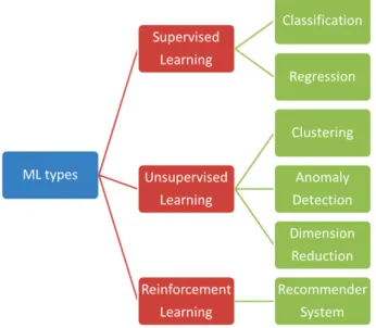
ML can be classified broadly in three types : supervised, unsupervi-sed and reinforcement learning. A fourth type is commonly accepted by some researcher as evolutionary learning1. In this thesis, we will focus on two most mature and commonly used ones, namely, supervised and unsupervised learning.
Figure 2.4 summarizes the most common ML types along with the most common tasks. Other supervised tasks are possible, though not represented in Figure 2.4, such as ranking and structural prediction for language translation.
Figure2.4 – Machine Learning types and different tasks type
Supervised learning. The key concept in supervised learning is la-beling. Let’s say we want to build an image cat detector system. First we collect as many images as possible and label manually each one as corresponding or not to a cat. We then train the machine by showing it the image and its corresponding label. We then create an objective func-tion that computes the error (or distance) between what the machine outputted and the expected value, i.e. the label. The machine then re-configures its internal ’knobs’ (known as ’weights’) to reduce the error accordingly. The typical tasks of supervised algorithms are classification and regression : predicting categories and numerical values respectively.
One limitation of this approach is the long and tedious work needed for labeling that data. We will delve into more details in the next section.
Unsupervised learning. Unsupervised learning maim goal is to des-cribe hidden structures from a given data input. Contrary to the super-vised learning, unsupersuper-vised learning doesn’t require labeled data. be-cause it does not have a clear target. Fundamentally, unsupervised lear-ning algorithms learn the data structure and characteristics. A common characteristic of unsupervised learning is the non-existence of accuracy metric. Unsupervised learning includes a broad range of algorithms that aim at reducing, transforming and describing the data such as K-means, Principal Component Analysis.
Other perspectives on ML algorithm can be : online and batch lear-ning. All these types are not mutually exclusive, for example an algo-rithm can be supervised and learns online.
Before exploring the depth of the ML approaches, we present a quick overview of the ML history in the next section.
C A Brief History of Machine Learning
Before the age of computer, philosophers have wondered whether it is possible for machines (or automatons at the epoch) to mimic human thoughts. Rene Descartes and Gottfried Wilhelm Leibniz in the 17th century, believed that human perceptions can be replicated using com-plex machines []. In the early 20th century Alan Turing demonstrated that any mathematical logic can be translated into a computer program []. He later in 1950 addressed the idea of a learning machine in [10] which predates genetic algorithms.
In the 50s, after the invention of the transistor and the first program-mable computers, these ideas could be tested which led to the inception of AI. Pioneering Machine Learning (ML) studies were conducted ba-sed on statistical methods ( e.g. Least squares, Bayes theorem, Markov chains) and simple algorithms. The first generation of AI researchers thought that AI problems are simple and that they could be resolved in few decades (Herbert Simon). However, they quickly realized the great complexity of such a task. In 1951, Marvin Minsky and Dean Edmonds created the first neural network capable of learning called the SNARC [11](page 105) but quickly realized its limitation (more on this point
in the ANN section in ??). In 1952, Arthur Samuel wrote the first pro-gram that learned from experience. A game of checkers that later beat its creator. The game learned to play against itself, as A. Samuel was very limited in term of resources he used a technique called Alpha-beta pruning2[12].
A few years later, in 1957, an influential paper on ML was introdu-ced by the mathematician Raymond Solomonoff [13]. He proposed a program that solves simple arithmetic problems by observing a sample of correct sequences. The machine learned to solve simple problems such as inferring the meaning of equality sign ‘=‘ from observing many sequences. R. Solomonoff used elementary “n-grams“ technique that consists of calculating the frequency of appearance of a given n letters and selecting the most frequent one.
In the subsequent years, many algorithms were created such as Nea-rest Neighbors, Turing’s Learning Machine and the introduction of back-propagation algorithm, i.e. the learning algorithm for neural networks. However the integration of ML solutions was hindered by the lack of data. Researchers didn’t access huge amount of data to perform training on.
In the 90s, when enormous amount of data was becoming available, the ML approach shifted from knowledge-driven to a data-driven ap-proach. In this period, Support Vector Machines and RNNs (and LSTMs in the late 90s) became popular. In this period of time, one limitation on ML was the training time necessary to train complex models. This led to using simpler models [14].
Another major limitation of ML algorithms was their ability to learn data in their raw format without feature engineering or domain exper-tise/knowledge. The solution was the representation learning approach which [15] consists of set of methods that allow the machine to automa-tically discover relevant features needed for detection. The most popu-lar one is deep learning [16]. In 2010s, the advances in GPUs manufac-turing and power, deep learning technique significantly improved ML tasks performance in many different domains. Deep Convolutional net-work revolutionized image processing [17], whereas recurrent netnet-works advanced progress in sequential data such as language translation[18].
The development of deep learning was reinforced by the development of many open-source ML frameworks. For instance, in 2015, Google re-leased the first version of TensorFlow.
Today, Deep learning is resolving major problems such as image, speech recognition thought to be insurmountable by AI. Deep learning success has expanded to particle accelerator analysis, drug discovery and DNA analysis [16]. Yet its performance is unquestionable in many tasks, we notice that its application for network and SLA management has not been sufficiently examined. We examined more thoroughly its applica-tion on some constrained applicaapplica-tion of network management in secapplica-tion ??. In the following section we will provide a more detailed view of ML supervised and unsupervised techniques. After that, we will discuss the current SOTA limitations.
II
Supervised Machine Learning
In supervised learning, the learning algorithm takes as input a vec-tor denoted x. This vecvec-tor consists of multiple training instances (or examples) denoted x(i), with i as the i(th) example. Each example has different attributes (or features) values denoted xj, with j as the j(th) fea-ture. The feature values can be either discrete (e.g. classes) or continuous (e.g. real numbers).
Thus we express xj as xj = (x(j)1 ; x(j)2 ; · · · ; x(j)i ; · · · ; xn(j)). Similarly we
de-note the jth corresponding labeled element as y(j) (also termed target or expected value). An observed example is the tuple (x(j); y(j)), meaning that when we observe x(j)we expect to get y(j). In table 2.1, the first observerd example is ((3; 50; 10); 200:000).
# of rooms (x1) Surface (m2) (x2) house age (x3) price (y = label)
3 50 10 200,000
5 200 5 500,000
6 500 25 1,100,000
Table2.1 – Labeled data example for a regression task.
clas-sification. We refer to each possible set of discrete value as a class. For example given an animal characteristics find which species it belongs to. The animal characteristics are the features and the species is the class.
If on the other hand, the output value is continuous, we call the task regression. For example, given the house characteristics find its price as presented in table 2.1. Based on the house features we would like to predict its price.
The training data correspond to the set of examples upon which the learning algorithm will learn and is denoted as Dtrain. The ML algorithm can be represented as a function f (also termed hypothesis H ) that maps the inputs to the outputs based on internal ’knobs’ ( or model parameters ). The model parameters can be thought of as the degree of contribution of a feature to the output. In the context of classification tasks f is commonly refered to as a classifier.
Common supervised algorithms are Linear Regression, Logistic Re-gression, Support Vector Machines (SVMs), Decision Trees and Artificial Neural Networks (ANNs). Note that the ANN can be used for regression, classification, unsupervised and reinforcement learning.
In order to illustrate all these points and definitions, we will use two examples, a very simple learning algorithm, namely linear regres-sion and a slightly more complex algorithm, Artificial Neural Networks (ANN).
Linear regression is simply an algorithm that fits the data using a linear function of form :
f (x) = 1:x + 2 (2.1)
Given a set of training data Dtrain depicted in figure 2.5, we would like to predict the y values of a given input x.
ML hyperparameter.In Machine Learning (ML) we distinguish bet-ween two configuration variables : the variables that can be inferred from the data, this is termed the model parameter and the configuration variables that cannot be estimated from the data distribution, termed the hyperparameters. The hyperparameters are considered as an inter-nal part of the ML models. They are generally set manually by the ML designer or require an intuition, using heuristics techniques.
Figure2.5 – Randomy generated data. the x-axis represent the input and y-axis repre-sents the target values.
Figure2.6 – Machine Learning types and different tasks type
The Case of ANN.
Artificial Neural Network (ANN) is a machine learning technique loosely inspired by the biological neural cells in the brain. A biological neuron figure ?? is composed of a cell body (nucleus In the figure) where most complex operations are performed. The branching extensions are called the dendrites. At the tip of the branches is a structure termed sy-napses. Biological neurons interact via electrical impulses called signals via the synapses. A neuron fires a signal when its total received signals exceed a certain threshold.
Figure2.7 – a Biological neuron [2]
The artificial counterpart of the biological neuron is what is termed a perceptron firstly developed by Frank Rosenblatt on an IBM 704 com-puter [19] inspired from early works in neuroscience
(a) fig 1 (b) fig 2
Figure2.8 – Artificial perceptron and its decision boundary
The perceptron takes inputs x (instead of binary values), perform some operations and outputs a signal y. As depicted in figure 2.8 each input is associated with a weight w that represents the importance of the input in the total calculation. The perceptron sums the weighted inputs plus a bias term z = wx + b is less than or greater than some thre-shold value (similar to Biological neuron). Similarity between biological and artificial neuron stops here. Biological neurons are far more com-plex than perceptron, and we continue to learn more and more of the
biological functions of neurons.
output =( 0 for Pixi:wi ≥threshold x for P
ixi:wi > threshold
(2.2)
The decision boudaty drawn by a neuron is represented in figure 2.8-b.
For the perceptron the decision boundary is :
W p + b = 0 The decision boundary of the perceptron is orthogonal to the weight vector. The perceptron can only draw lineraly separable decision boundaries.
Perceptrons are linear transformers, they can only split the data li-nearly. This limitation was pointed out by Marvin Minsky and Seymour Papert in [20].This caused the researches to drop and lose interest in the ‘connectionist‘ approach. More specifically, they pointed out that perceptron cannot learn XOR function (later termed the XOR problem). This problem is illustrated in figure 2.9 one cannot draw a straight line to separate + from -. As a result, the research community lost interest in ANN for several years.
A B A XOR B
0 0 0
0 1 1
1 0 1
1 1 0
Figure2.9 – Non-linear decision boundary XOR
Figure2.10 – MLP solving XOR problem
Figure2.11 – MLP solving XOR problem
The XOR problem was solved using and OR and an not AND in the hidden layer and an AND gate in the output layer.
A B (A OR B) AND (A !AND B)
0 0 = 0
0 1 1
1 0 1
1 1 0
Table2.3 – Exclusive OR : XOR Truth table
Later, this limitation was eliminated by stacking multiple trons together. This configuration is what we call Multi-Layered Percep-tron (MLP). The layers between the input layer and the output layer is what we call the hidden layers. in the human brain there exits 1011 neu-rons of 20 types
Figure2.12 – simple MLP example
Example MLP.
We will use an MLP example as represented in Figure 2.12 throu-ghout this section in order to illustrate the basic principles behind MLP. The MLP is a 3-layered ANN, with two input units and one output. The hidden layer is composed of three units. The link between each neu-ron is refered to as a synapse.
More formally, the synapses parameters are termed weights W . W(1)
se-cond layer respectively. X = 2 6 6 6 6 6 6 6 6 6 6 6 6 6 4 X1(1) X2(1) X1(2) X2(2) · · · · X1(n) X2(n) 3 7 7 7 7 7 7 7 7 7 7 7 7 7 5 (2.3)
, where n is the number of examples.
W(1)= 2 6 6 6 6 4 W11(1) W12(1) W13(1) W21(1) W22(1) W23(1) 3 7 7 7 7 5 (2.4) W(2) = 2 6 6 6 6 6 6 6 6 6 4 W11(2) W21(2) W31(2) 3 7 7 7 7 7 7 7 7 7 5 (2.5)
Instead of the step function defined previously we used the sigmoid function as the activation function. We will explain in the learning phase the reason behind this choice.
The sigmoid function is a function that maps inputs from [− inf; inf] to values from 0 to 1, [0; 1]. it is defined as follows3 :
f (x) = 1
1 + e−x (2.6)
Prediction.
The nominal behavior of the ANN is taking the inputs from the input layers, through hidden layers to the output. This is called the forward pass. In this section, we will follow/describe this process using matrix notation along with the resulting matrix shape. The matrix notation are very helpful in that it summarizes in one line the operations for each neuron. We used Z and A to refer to the weighted sum and the applied activation function over the result respectively (if confused see figure 2.12).
From the input layer to the hidden layer :
Multiplying the inputs by the hidden layer weights :
Z(2) = X:W(1) (2.7)
, where X size is (n ∗ 2) and W(1) is (2 ∗ 3), resulting in Z(2) of size (n ∗ 3). Then applying the activation function :
A(2) = f (X:W(1)) = Z(2) (2.8) , A(2) is the output of the activation function and the input of the output and final layer.
Again, the same operation from the hidden layer to the output layer :
Z(3) = A(2):W(2) (2.9)
, where A(2) size is (n ∗ 3) and W(3) is (3 ∗ 1), resulting in Z(3) of size (n ∗ 1). This means that for each input (i.e. each X row) we get one output.
Applying the activation function :
A(3) = f (X:W(1)) = f (Z(3)) = ˆy (2.10) , A(3) is the outputed result. We will refer to it as ˆy(i) with i as ith output corresponding to the ith input (X(i)). In matrix notation ˆy = A(3).
A How machines learn.
The fundamental objective of learning is to generalize. This means that the algorithm should obtain good performance not only with res-pect to the training examples but also over new samples never seen be-fore.
Conceptually, we splitted the two concerns into two sections. (1) Ob-taining good performance over the training set and (2) generalizing to new examples. For sake of completeness and simplicity, we dedicate this section “How machine learn“ to the first point. We will then tackle the second point in section ??. Notice that the (1) and (2) are fundamentally opposed. improving (1) hinders (2) and vice-verca. More details on this point later in this chapter.
Machines learn by finding a function f that maps the outputs y to the input x with the minimun error possible. In other words, learning is akin to optimizing a cost function. To this end, we define for each pair of output, label, i.e. (y(i); ˆy(i) = f (Xi)) aloss function. The loss function mea-sures the distance between the label (expected value or ground-truth)
and the outputted value. Typically, a loss function is defined as the squa-red difference between the two values as follows :
Loss(i) = Loss(( ˆy(i); y(i))) = (f (Xi) − y(i))2 (2.11) From the loss function, we determine thecost function which is a more general term than the loss function. Learning from data means minimi-zing the cost function. Often, the cost function is computed by avera-ging over the losses of all the training examples. This is called the Mean Squared Error (MSE).
MSE( ) = 1 N n X i=1 Loss(i) = J( ) (2.12)
, the cost function is usually refered to as J( )
Back to our linear regression example, in order to compute J( ) we should start with an initial set (or coefficients). We can initialize these coefficients randomly, then proceed in tuning them to reduce J( ) to its minimum.
Gradient Descent (GD).
Figure2.13 – Gradient Descent
We have described in equation 2.13 a method to compute the cost function. Now, we would like to try different parameters to find the optimal J( ). Trying all the possible model parameters might seem sen-sible, however, the curse of dimensionality prevent us from doing so,
because of the large explosion of all the possible combinations. A more practical strategy is to compute the cost function derivative to find the direction that decreases the cost. This optimization method is called Crandient Descent (GD) A key parameter in this phase is the leanring rate or the step size ( in figure 2.14). if the step size is too small, the algorithm may take a long time to converge (figure 2.14 left). Conversly, if the step size is too large the algorithm might bounce from one end to another without converging (figure 2.14 right).
”It simply starts at an initial point and then repeatedly takes a step opposite to the gradient direction of the function at the current point. The gradient descent algorithm to minimize a function f (x) is as fol-lows :”
Algorithm 1:Gradient Descent algorithm
Data: Get the training data, DT rain
Result: Return optimal model parameters j
1 initialization; 2 j = 0; 3 repeat 4 read current; 5 Update. j := j− :∇ J( 0; 1) (f or j = 0 and j = 1) 6 until Convergence;
, with asthe step size and ∇wJ( ) as the gradient
GD is an iterative optimization technique that starts at some initial points (i.e. ), it changes w so that the cost function value decreases, guranteeing the lowest error. The gradient of the cost function comes in handy, because it allows us to determine the slope of the function, it is very practical when working in higher dimensions in order of hundred of thoudands. The GD has two hyperparameters ; namely the step size and the number of iteration T .
determines how the aggressive is the algorithms moves if it is set too low or too high see figure 2.14.
T is the number of iterations. each iteration requires going over all training examples - expensive when have lots of data ! Another problem is that it is slow.
GD is slow. There exists many optimization algorithm such as Sto-chastic Gradient Descent that instead of taking the gradient of the cost
function it uses the gradient of the loss function. SGD updates the weight based on each single example (x; y) instead of all examples. Empirically, SGD performs as well as GD in on epass over all the example as GD in 10 epochs[].
Other optimization method exists, we refer the reader to xxx [] for more details. MSE( ) = 1 N n X i=1 Loss(i) = J( ) (2.13)
Figure2.15 – Optimizer comparison
”In addition to local minima and the (rare) possibility of getting stuck at a saddle point, there are other issues that should be taken into consi-deration.
For example, if the step size tk remains large, it may lead to an oscil-latory behavior that does not converge.
Another issue is that, depending on the function and starting point, gradient descent could continue indefinitely because there is no mini-mum. Consider for example minimizing ex: there is no finite x for which
d
dxex = 0. Other functions could have such asymptotic minima but also
a global minimum of lower value ; gradient descent, depending on its starting point, might forever chase the asymptote, unaware of the true answer elsewhere in the search space.”
The case of the ANN.
The perceptron training algorithm was inspired by Donald Hebb in [21]. Hebb proposed a theory that explains the learning process in the brain. The idea was later summarized as “Cells that fire together, wire together“, this means that in the learning process, the neurons that are stimulated together reinforce their mutual connection. ANNs are
trai-ned using a similar approach, more specifically, for each wrong pre-diction, the training algorithm reinforce the weights that would have contributed to the correct answer. More formally we write :
perceptron learning rule w(new) = w(old) + ep ep = t - a
In the literature, researchers have struggled for many years to train the MLP. In 1986, D. Rumelhart et al. [22] introduced backpropagation algorithm. Rumelhart et al. tackled the XOR problem upfront and de-monstrated that with their procedure the network can learn to solve the XOR. Backpropagation caused the second resurgency of connectionism
For each training instance, the ANN computes the output this is cal-led the forward pass. Then the algorithm computes the distance between the expected output and the output. Then, calculate the contribution of hidden layer to the overall error. By propagating the error from the out-put layer to the hidden layers and to each neuron in the hidden layer. Then it modifies the weight in the opposite direction of the gradient for each neuron. More specifically, it propagates the error gradient back-wards, thus the name backpropagation. Rumelhart et al. remplaced the standard step function with the logistic activation function s(z) in order for the backpropagation to work. The standard step functions contains only constant values, the derivative is then always null and cannot be used to compute the gradients as in Figure 2.16 in red. Whereas the Lo-git function has nonzero derivatives see figure 2.16 green
In order to simplify the backpropagation algorithm we will continue with our small MLP of one hidden layer :
Training of the ANN.
It means to optimize the network weights ij1; ij2) in order to mini-mize the cost function J( ). In this paper, the Backpropagation algo-rithm is used to train the ANN. For each training vector x((i)) and label vector y(i) : J( ) = N X i=1 1 2:( ˆy − y) 2 (2.14)
In order to apply Gradient Descent algorithm we should compute the cost function gradients with respect to W(1) and W(2) :
dJ dW(1) = 2 6 6 6 6 6 6 6 6 6 6 6 4 dJ dW11(1) dJ dW12(1) dJ W13(1) dJ dW21(1) dJ dW22(1) dJ dW23(1) 3 7 7 7 7 7 7 7 7 7 7 7 5 (2.15) dJ dW(2) = 2 6 6 6 6 6 6 6 6 6 6 6 6 6 6 6 6 6 6 6 6 6 6 6 4 dJ dW11(2) dJ dW21(2) dJ dW31(2) 3 7 7 7 7 7 7 7 7 7 7 7 7 7 7 7 7 7 7 7 7 7 7 7 5 (2.16)
Let’s start with dJ
dW(2), dJ dW(2) = dPN i=112:( ˆy − y)2 dW(2) (2.17)
Recall rule 1. The sum of the differentiation : d(U + V ) dx = dU dx + dV dx (2.18)
For one training example we have : dJ
dW(2) =
d12:( ˆy − y)2
dW(2) (2.19)
Recall rule 2. The power rule : d(Un)
dx = n:U
n−1 (2.20)
Recall rule 3. The chain rule : dy dx = dy dz: dz dy (2.21)
Figure2.16 – Activation functions and their respective derivatives
Using rule 2 and rule 3 in equation 2.19, we get :
dJ dW(2) = d12:( ˆy − y)2 d(y − ˆy) : d(y − ˆy) dW(2) = (y − ˆy):d(y − ˆy) dW(2) y = cte ⇒ dy dW(2) = 0 = (y − ˆy): −d ˆy dW(2) (2.22)
From equation 2.10, we have f (Z(3)) = ˆy and using rule 3 : dJ dW(2) = −(y − ˆy): d ˆy dZ(3): dZ(3) dW(2) (2.23)
we have f (z) = 1+e1−z and f
0
(z) = (1+ee−−zz
)2 see figure 2.16. we replace
d ˆy dZ(3) by f 0(Z(3)) since f (Z(3)) = ˆy. dJ dW(2) = −(y − ˆy):f 0 (Z(3)): dZ (3) dW(2) (2.24)
Notice that in equation 2.24 the term −(y − ˆy):f0(Z(3)) represents the gradient error propagated to the synapses in the hidden layers. The mul-tiplication is interpreted as the weights with highest values get the hi-ghest blame for the error. This term is usually referd to as the gradient error (3). The step function previously used as the activation function in the first ANNs does not work in this case since its derivative remains
null. It is for this reason that the researchers switched from threshold activation function to the sigmoid see figure 2.16.
For the term dZ(3)
dW(2), we have from equation 2.9 Z
(3) = A(2):W(2). Thus we have : dZ(3) dW(2) = dA(2):W(2) dW(2) = A(2) (2.25)
We replace the terms in equation 2.24 while transposing the A(2) ma-trix to respect the dimensions :
dJ
dW(2) = (A
(2))T: (3) (2.26)
The matrix transposed and multiplication takes account for all the training examples. We have (3 ∗ nexamples) for (A(2))T and (nexamples ∗ 1) which equals to a (3 ∗ 1) matrix size with 3 as the number of hidden layers.
The equation 2.26 is propagating the error from the output layer to the hidden layer. Each synapse gets its share of the error. Next step, we will show how the error is propagated back from the hidden layer to the synapses in the input layer. To do so, we will compute dJ
dW(1). dJ dW(1) = dPN i=112:( ˆy − y)2 dW(1) (2.27) similarly to dJ dW(2) in equation 2.24 we get : dJ dW(1) = −(y − ˆy):f 0 (Z(3)):dZ (3) dW(1) (2.28) dJ dW(1) = (3):dZ(3) dW(1) (2.29)
For the term dZ(3)
dW(1) in equation 2.28, we now from equation 2.9 that
Z(3)= A(2):W(2). Thus, we write : dJ dW(1) = (3):dZ(3) dA(2): dA(2) dW(1) (2.30)
We replace dZdA(3)(2) = dAdA(2):W(2)(2) = W(2) dJ
dW(1) =
(3):(W(2))T:dA(2)
dW(1) (2.31)
And we have for the term dWdA(2)(1), from equation 2.8, A(2) = f (Z(2)). we write using rule 3 and insering Z(2) :
dJ dW(1) = (3):(W(2))T:dA(2) dZ(2): dZ2 W(1) (2.32)
We have this term dA(2)
dZ(2) = f 0 (Z(2)) and dZ2 W(1) = dX:W(1) W(1) = X Finally we write : dJ dW(1) = (X) T: (3):(W(2))T:f0 (Z(2) (2.33)
We refer to the term (3):(W(2))T:f0(Z(2) as (2) the gradient error pro-pagated to the synapses in the input layer.
Using equation 2.33 and 2.26, we can compute the Gradient Descent as follows : 2 6 6 6 6 6 6 6 6 6 6 6 4 1 2 3 7 7 7 7 7 7 7 7 7 7 7 5 = 2 6 6 6 6 6 6 6 6 6 6 6 4 1 2 3 7 7 7 7 7 7 7 7 7 7 7 5 − 2 6 6 6 6 6 6 6 6 6 6 6 6 6 4 dJ dW(1) dJ dW(2) 3 7 7 7 7 7 7 7 7 7 7 7 7 7 5 (2.34)
, with as the gradient step size and J as a differentiable cost function.
B Evaluation
Machine Learning diagnosis : Bias and Variance
Failing to generalize can have two forms. First, not being capable of learning the complexity of the objective function, termed underfitting or bias, figure 2.20. Second, learning too much the data characteris-tics,figure 2.20. A common misconception about overfitting is that the ML algorithm learns the noise in the data. But serious overfitting can be caused without noisy data (e.g. maybe give an example, 40th order polynomial) [14].
In this section, we will take the example of a classifier that tries to detect sick patients from a population. we refer to the population size as N . We refer to the sick patients as P ositive or P and the Healthy patients as N egative or T N . We set N = 100, and the ground-truth is P = 5, N = 95. When an algorithm classifies a patient into positive or negative, we denote Palgo, Nalgo respectivelly.
Figure2.17 – bias vs variance
The evaluation of ML algorithm aims to assess how good or bad the evaluation generalizes to new results never seen before. To this end, a basic methodology in ML is to split the data into two sets, a training set on which to train the algorithm and a test set that represents new data on which to test the generalization capabilities.
There exist other techniques to detect and combat generalization pro-blems, we will discuss them in the following sections. In the case of bias the algorithm scores poorly on the training data. In the second case, the algorithm gets a high score on the training set but scores poorly on the test or valisation data set.
Before delving into how to avoid bias and variance, we will define common evaluation metrics with examples for each one to demonstrate the importance of each one.
![Figure 1.1 – The cost of hardware and software and their management [1].](https://thumb-eu.123doks.com/thumbv2/123doknet/11500655.293623/23.892.304.601.197.457/figure-cost-hardware-software-management.webp)