HAL Id: hal-00177572
https://hal.archives-ouvertes.fr/hal-00177572
Submitted on 8 Oct 2007
HAL is a multi-disciplinary open access
archive for the deposit and dissemination of sci-entific research documents, whether they are pub-lished or not. The documents may come from teaching and research institutions in France or abroad, or from public or private research centers.
L’archive ouverte pluridisciplinaire HAL, est destinée au dépôt et à la diffusion de documents scientifiques de niveau recherche, publiés ou non, émanant des établissements d’enseignement et de recherche français ou étrangers, des laboratoires publics ou privés.
Emmanuel Moulay, Wilfrid Perruquetti
To cite this version:
Emmanuel Moulay, Wilfrid Perruquetti. Finite time stability conditions for non autonomous con-tinuous systems. International Journal of Control, Taylor & Francis, 2008, 81 (5), pp.797-803. �10.1080/00207170701650303�. �hal-00177572�
International Journal of Control Vol. 00, No. 00, January 2006, 1–12
Finite time stability conditions for non autonomous continuous systems
E. MOULAY∗† and W. PERRUQUETTI‡
†IRCCyN (UMR-CNRS 6597), 1 rue de la No¨e, BP 92 101, 44321 Nantes Cedex 03, FRANCE
‡ LAGIS (UMR-CNRS 8146), Ecole centrale de Lille, Cit´e Scientifique, 59651 Villeneuve d’Ascq Cedex, FRANCE
(submitted 21/06/2004, revised 16/06/2006)
Finite time stability is defined for continuous non autonomous systems. Starting with a result from Haimo Haimo (1986) we then extend this result to n−dimensional non autonomous systems through the use of smooth and nonsmooth Lyapunov functions as in Perruquetti and Drakunov (2000). One obtains two different sufficient conditions and a necessary one for finite time stability of continuous non autonomous systems.
1 Introduction
Since the end of the 19thand the beginning of the 20thcentury, various concepts dedicated to the qualitative behavior of the solutions for dynamical systems have been introduced (for example the seminal definitions and results from A.M. Lyapunov Lyapunov (1992)). But rapidly, one had to face some more precise time specifications of the behavior of the state variables (or outputs) for real process. For example, some finite time stabilizing control design relies upon sliding mode theory (see Utkin (1992)) and another one upon optimal control theory (see Ryan (1979)). In both cases the controller leads to some state discontinuous feedback control laws. Over the years much work has been dedicated to this concept, getting some sufficient conditions and the application to the construction of finite-time stabilization control (see for example Bhat and Bernstein (1998), Hong (2002), Hong et al. (2001, 2002), Moulay and Perruquetti (2006a)). The main idea lies in assigning infinite eigenvalue to the closed loop system at the origin. Let us mention the following illustrative example
˙x = − |x|asgn(x), x ∈R, a ∈ ]0, 1[ , (1)
for which the solutions starting at τ = 0 from x are:
φx(τ ) = sgn(x)³|x|1−a− τ (1 − a)´ 1 1−a ) if 0 ≤ τ ≤ |x|1−a1−a 0 if τ > |x|1−a1−a , (2)
and they reach the origin in finite time. In fact, there exists a function called settling time that increases the time for a solution to reach the equilibrium. Usually, this function depends on the initial condition of a solution. But, for non autonomous systems, it may also depend on the initial time. Lastly, notice from this example, that in order to obtain finite time stability, the right hand side of the ordinary differential equation cannot be locally Lipschitz at the origin.
The paper is organized as follows. After defining the notion of finite time stability for continuous non autonomous systems in section 2 , we recall the necessary and sufficient conditions for finite time stability of autonomous scalar systems (section 3) (result which appears in Haimo (1986), Moulay and Perruquetti (2006b) and whose proof is given here. Then in section 4, we give a generalization for continuous non ∗Corresponding author. Email: [email protected]
International Journal of Control
ISSN 0020-7179 print/ISSN 1366-5820 online c°2006 Taylor & Francis http://www.tandf.co.uk/journals
autonomous systems of any dimension. For this we introduce a Lyapunov function whose derivative satisfies an increase to obtain sufficient conditions for finite time stability. In the subsection 4.1, one uses a smooth Lyapunov function and in the subsection 4.2, one uses a nonsmooth one. Nevertheless, as we will see the use of a smooth Lyapunov function is not a weaker result, only a different one. Then, a Lyapunov function whose derivative verifies a decrease is used in order to obtain necessary conditions for finite time stability (see subsection 4.3).
Through the paper, the following notations will be used:
• for a > 0, the following function will be used ϕa(x) = |x|asgn(x),
• V denotes a neighborhood of the origin inRn ,
• Bǫ is the open ball centered at the origin of radius ǫ > 0.
The upper Dini derivative of a function f :R → R is the function D+f :R → R defined by: D+f(x) = lim sup
h→0+
f(x + h) − f (x)
h .
2 What is finite time stability?
Consider the system
˙x = f (t, x), t∈R≥0, x∈Rn, (3)
where f : R≥0 ×Rn → Rn is a continuous function. Then φxt (τ ) denotes a solution of the system ( 3)
starting from (t, x) ∈R≥0×Rn and S (t, x) represents the set of all solutions φxt. The existence of solutions
is given by the well known Cauchy-Peano Theorem given for example in Hale (1980). A continuous function α: [0, a] → [0, +∞[ belongs to class K if it is strictly increasing and α(0) = 0. It is said to belong to class K∞ if a = +∞ and α(r) → +∞ as r → +∞. Moreover, a continuous function V :R≥0× V →R≥0 such
that
L1) V is positive definite, L2) ˙V(t, x) = D+³V ◦ ˜φx t
´
(0) is negative definite with ˜φxt (τ ) = (τ, φx t(τ )),
is a Lyapunov function for (3). If V is smooth then ˙ V(t, x) =∂V ∂t(t, x) + n X i=1 ∂iV ∂xi (t, x)fi(t, x).
A continuous function v :R≥0× V →R is decrescent if there exists a K− function ψ such that
|v(t, x)| ≤ ψ (||x||) ∀(t, x) ∈R≥0× V.
A continuous function v :R≥0×Rn→R is radially unbounded if there exists a K∞−function ϕ such that
v(t, y) ≥ ϕ(||y||), ∀t ∈R≥0 ∀y ∈Rn.
The definition of asymptotic stability is well known (see Hahn (1963)). In this case, the solutions of the system (3) tend to the origin (but without information about the time transient). This information comes from the notion of “settling time” which, when finite and combined with the stability concept, leads to the following definition for finite time stability
A1) the origin is Lyapunov stable for the system (3),
A2) for all t ∈ I, there exists δ(t) > 0, such that if x ∈ Bδ(t) then for all Φxt ∈ S (t, x):
a) φx
t(τ ) is defined for τ ≥ t,
b) there exists 0 ≤ T (φx
t) < +∞ such that φxt(τ ) = 0 for all τ ≥ t + T (φxt).
T0(φxt) = inf{T (φxt) ≥ 0 : φxt(τ ) = 0 ∀τ ≥ t + T (φxt)}
is called the settling time of the solution φx t.
A3) Moreover, if T0(t, x) = sup φx
t∈S(t,x)
T0(φxt) < +∞, then the origin is finite time stable for the system (3).
T0(t, x) is called the settling time with respect to the initial conditions of the system (3).
Remark 1 When the system is asymptotically stable, the settling time of a solution may be infinite. If the system (3) is continuous on I × V and locally Lipschitz on I × V \ {0}, because of solution uniqueness, the settling time of a solution and the settling time with respect to the initial conditions of the system are the same: T0(t, x) = T0(φxt).
Definition 2.2 Let the origin be an equilibrium point of the system (3). The origin is uniformly finite time stable for the system (3) if the origin is
B1) uniformly asymptotically stable for the system (3), B2) finite time stable for the system (3),
B3) there exists a positive definite continuous function α : R≥0 → R≥0 such that the settling time with
respect initial condition of the system (3) satisfies:
T0(t, x) ≤ α (kxk) .
3 Autonomous scalar systems
Let us recall the result for finite time stability of autonomous scalar systems of the form
˙x = f (x), x∈R, (4)
where f : R → R given in Haimo (1986). In this particular case there exists a necessary and sufficient condition for finite time stability:
Lemma 3.1 Let the origin be an equilibrium point of the system (4) where f is continuous. The origin is finite time stable for the system (4) if and only if there exists a neighborhood of the origin V such that for all x ∈ V \ {0} xf(x) < 0, (5) Z 0 x dz f(z) <+∞. (6)
Proof (⇐) As xf (x) < 0, V (x) = x2 is a Lyapunov function for the system. So, the origin of the system
(4) is asymptotically stable.
Let φx(τ ) be a solution of the system which tend to the origin with time T (φx). We have to show that
T(φx) < +∞. With the asymptotic stability, if x is small enough, then τ 7→ φx(τ ) is strictly monotone for
Moreover, T(φx) = Z T(φx) 0 dτ. As xf (x) < 0 for all x ∈ V\{0}, 1
f is defined on V\{0}. The following change of variables, [0, T (φ
x)[ → ]0, x], τ 7→ φx(τ ) leads to Z 0 x dz f(z) = Z T(φx) 0 ˙ φx(τ ) f(φx(τ ))dτ = T (φ x) < +∞. T(x) = sup φx∈S(x)
T(φx) does not depend on φx. So, we conclude that the origin of the system (4) is finite
time stable with the following settling time T0(x) = T (φx) satisfying T0(x) =
Z 0
x
dz f(z).
(⇒) Suppose that the origin of the system (4) is finite time stable. Let δ > 0 given by definition 2.1. Suppose that there exists x ∈ ]−δ, δ[ \ {0} such that xf (x) ≥ 0.
• If xf (x) = 0, then f (x) = 0 et φx(τ ) ≡ x is a solution of the system (4) which does not tend to the origin.
• If xf (x) > 0, with no loss of generality, we can suppose that x > 0 et f (x) > 0. The continuity of f and the fact that f (x) > 0 lead to f (z) > 0 for z in a neighborhood of x. Then, the function τ 7→ φx(τ )
increases in a neighborhood of the origin. With its continuity, this solution can not tend to the origin. Let x ∈ ]−δ, δ[ \ {0} and consider the solution φx(τ ). By assumption, there exists 0 ≤ T
0(φx) < +∞
such that φx(τ ) = 0 for all τ ≥ t + T
0(φx). With the asymptotic stability, x can be chosen small enough
such that τ 7→ φx(τ ) decreases for τ ≥ t. The following change of variables [0, T
0(φx)[ → ]0, x], τ 7→ φx(τ ) leads to Z 0 x dz f(z) = Z T0(φ x ) 0 dτ = T0(φx) < +∞. ¤
For x in a neighborhood of the origin, the settling time of a solution of (4) and the settling time with respect to the initial conditions of the system (4) are equal and
T0(x) =
Z 0
x
dz f(z).
If the system (4) is globally defined and if conditions (5) and (6) hold globally, then the origin is globally finite time stable. Moreover, it is obvious that for autonomous systems, uniform finite time stability is finite time stability.
Example 3.2 Let a ∈ ]0, 1[ and consider system (1). Obviously −xϕa(x) < 0 for x 6= 0, and let x ∈ R
then Z 0 x dz − |z|asgn(z) = |x|1−a 1 − a <+∞.
The assumptions of Lemma 3.1 are satisfied. Thus the origin is uniformly finite time stable and the solutions φx(τ ) tend to the origin with the settling time T0(x) = |x|
1−a
1−a . These conclusions were directly obtained in
4 General case
For the more general systems described by Equation (3), a natural extension will invoke the use of Lyapunov functions to give sufficient or necessary conditions for finite time stability.
4.1 Sufficient condition using smooth Lyapunov function
In this section, we extend a result coming from Haimo (1986) to non autonomous systems. In the following, one needs the existence of a Lyapunov function V :R≥× V →R≥ and a continuous function r :R≥→R≥
such that r (0) = 0 satisfying the following differential inequality ˙
V(t, x) ≤ −r (V (t, x)) (7)
for all (t, x) ∈ I × V.
Since the use of a Lyapunov function will lead to some scalar differential inequality, the following proposi-tion will give sufficient condiproposi-tion for finite time stability: the existence of a Lyapunov funcproposi-tion satisfying the condition (7).
Proposition 4.1 Let the origin be an equilibrium point for the system (3) where f is continuous. i) If there exists a continuously differentiable Lyapunov function satisfying condition (7) with a positive
definite continuous function r :R≥0 →R≥0 such that for some ǫ > 0
Z ǫ
0
dz
r(z) <+∞ (8)
then the origin (3) is finite time stable for the system (3).
ii) If in addition to i), V is decrescent, then the origin of the system (3) is uniformly finite time stable for the system (3).
iii) If in addition to i), the system (3) is globally defined and V is radially unbounded, then the origin of the system (3) is globally finite time stable for the system (3).
Proof i) Since V : I × V → R≥0 is a Lyapunov function (thus satisfies L1 and L2), then the Lyapunov
Theorem tells us that the origin is asymptotically stable. Let φx
t (τ ) be a solution of (3) which tends to
the origin with the settling time T0(φxt (τ )) (0 ≤ T0(φxt(τ )) ≤ +∞ : from the attractivity of the origin).
We have to prove that T0(t, x) < +∞. By using the asymptotic stability definition, x can be chosen small
enough to ensure that φx
t (τ ) ∈ V for τ ≥ t and τ 7→ V (τ, φxt (τ )) strictly decreases for τ ≥ t. By using the
change of variables: [t, t + T0(φxt)] → [0, V (t, x)] given by z = V (τ, φxt (τ )), one obtains
Z 0 V(t,x) dz −r(z) = Z t+T0(φ x t) t ˙ V(τ, φx t (τ )) −r(V (τ, φx t (τ ))) dτ.
By assumption, ˙V(τ, φxt (τ )) ≤ −r(V (τ, φxt (τ ))) ≤ 0 for all τ ≥ t. This shows that
T0(φxt) = Z t+T0(φ x t) t dτ ≤ Z V(t,x) 0 dz r(z).
This implies that T0(φxt) < +∞. As
Z V(t,x)
0
dz
r(z) is independent of φ
x
t, T0(t, x) < +∞. Thus, the origin of
the system (3) is finite time stable.
K−function β such that V (t, x) ≤ β (kxk). So T0(t, x) ≤ Z β(kxk) 0 dz r(z) = α (kxk) with α positive definite.
iii) If V is radially unbounded, the system is globally asymptotically stable. Then, for all x inRn all the
functions τ 7→ V (τ, φxt (τ )) decrease. Thus the system is globally finite time stable. ¤
Remark 1 The settling time with respect to initial conditions of the system (3) satisfies the following inequality T0(t, x) ≤ Z V(t,x) 0 dz r(z). so it is continuous at the origin.
Example 4.2 Scalar non autonomous systemConsider the following system:
˙x = −(1 + t)ϕa(x), t≥ 0, x ∈R. (9)
The function V (x) = x2 is a decrescent Lyapunov function for (9) and
˙ V(t, x) = −2(1 + t)xϕa(x) ≤ −2ϕa+1 2 (x2) = −r(V (x)). Since Z ǫ 0 dz
r(z) <+∞, the origin is uniformly finite time stable with the settling time with respect to initial conditions of the system
T0(t, x) ≤
4 |x|1−a 1 − a .
Example 4.3 two dimensional systemConsider a ∈]0, 1[ and the system: ½ ˙x1 = −ϕa(x1) − x31+ x2 ˙x2 = −ϕa(x2) − x32− x1. Taking V (x) = kxk22,we obtain ˙ V (x1, x2) = − 2 X i=1 (x4i + |xi|a+1) ≤ 0.
V is a Lyapunov function for the system. Moreover, if r (z) = ϕa+1 2 (z), then ˙ V (x1, x2) ≤ −r (V (x1, x2)) . In fact 2 X i=1 (x4i + |xi|a+1) ≥¡x21+ x22 ¢a+12 = kxka+1.
Thus the origin is uniformly finite time stable with T0(t, x) ≤ 2 1+a 2 kxk1−a 1 − a .
In order to test condition (8) and to conclude to the finite time stability, first one must have the existence of a pair (V, r) satisfying condition (7). For this, it is enough that there exists a decrescent Lyapunov function for the system (3). Indeed, if V is decrescent, then there exists a class K-function α such that
V(t, x) ≤ α (kxk)
for all (t, x) ∈R≥0× V. As ˙V is negative definite, there exists a class K-function β such that
− ˙V(t, x) ≥ β(kxk) for all (t, x) ∈R≥0× V. Combining both results, one obtains that
˙
V(t, x) ≤ −β¡α−1(V (t, x))¢
for all (t, x) ∈R≥0× V. Note that this condition does not imply that the constructed pair (V, r) will be a
good candidate for condition (8).
4.2 Sufficient condition using nonsmooth Lyapunov function
The question is to know if it is possible to use a continuous only Lyapunov function to show finite time stability. This is possible by adding the condition that r is locally Lipschitz. We shall use the comparison lemma which can be found in (Khalil 1996, Lemma 3.4):
Lemma 4.4 Comparison lemmaIf the scalar differential equation ˙x = f (x), x∈R,
has a global semi-flow Φ :R≥0×R → R, where f is continuous, and if g : [a, b) → R (b could be infinity)
is a continuous function such that for all t ∈ [a, b),
D+g(t) ≤ f (g(t)) then g(t) ≤ Φ(t, g(a)) for all t ∈ [a, b).
Now, one may give a proposition which generalizes a result given in Bhat and Bernstein (2000) to continuous non autonomous systems.
Proposition 4.5 Let the origin be an equilibrium point for the system (3) where f is continuous. If there exists a continuous Lyapunov function for the system (3) satisfying condition (7) with a positive definite continuous function r :R≥0 →R≥0 locally Lipschitz outside the origin such that R0ǫr(z)dz <+∞ with ǫ > 0,
then the origin is finite time stable. Moreover, the settling time with respect to initial conditions of the system (3) satisfies T0(t, x) ≤ Z V(t,x) 0 dz r(z).
Proof Since V : R≥0× V → R≥0 is Lyapunov function of the system (3) satisfying condition (7), then
of (3) which tends to the origin with the settling time T0(φxt). It remains to prove that T0(t, x) < +∞.
Because of asymptotic stability, one may suppose with no loss of generality that φx
t (τ ) ∈ V for t ≥ 0 and
V(t, x) ∈ [0, ǫ]. Let us consider the system
˙z = −r(z), z≥ 0,
with the global semi flow Φ(τ, z) for z ≥ 0. Now, applying the comparison lemma (4.4), one deduces that V (τ, φxt(τ )) ≤ Φ(τ, V (t, x)), τ ≥ 0, x ∈ V \ {0} .
From Lemma 3.1, one knows that
Φ(τ, z) = 0 for τ ≥
Z V(t,x)
0
dz r(z). With the positive definiteness of V , one concludes that
φxt (τ ) = 0 for τ ≥ Z V(t,x) 0 dz r(z). Moreover, Z V(t,x) 0 dz r(z) is independent of φ x
t, this shows that T0(t, x) < +∞. Thus, the origin of the system
(3) is finite time stable. ¤
One wants to give an example using a continuous only Lyapunov function. Example 4.6 Let 0 < a < 1, if we consider the simplest system
˙x = −xasgn(x), x∈R, and the continuous Lyapunov function V (x) = |x|, we have
˙
V(x) = − |x|a= −V (x)a. So the system is finite time stable.
Let us sum up the two previous results: in order to obtain the finite time stability, we have the choice between a pair (V1, r1) with V1which is continuously differentiable and r1 only continuous, or a pair (V2, r2)
with V2 which is continuous and r2 locally Lipschitz. Moreover, the two conditions are not equivalent
because there is no converse theorem for general non autonomous continuous systems.
4.3 Necessary conditions
For the moment, there is no necessary and sufficient condition for finite time stability of general contin-uous (even autonomous) systems. The only converse theorem appears in Bhat and Bernstein (2000) for autonomous systems with uniqueness of solutions in forward time and when the settling time is continu-ous at the origin. So, one proposes a sufficient condition for non autonomcontinu-ous continucontinu-ous systems. In the following, one needs the existence of a Lyapunov function V :R≥× V → R≥ and a continuous function
s:R≥ →R≥ such that s (0) = 0 satisfying the following differential inequality
˙
V(t, x) ≥ −s(V (t, x)) (10)
for all (t, x) ∈R≥0× V. Then, the following proposition gives necessary conditions for finite time stability:
Proposition 4.7 Let the origin be an equilibrium point for the system (3) where f is continuous. If the origin is weakly finite time stable for the system (3) then for all Lyapunov functions for the system (3) satisfying condition (10) with a continuous positive definite function s : R≥0 → R≥0, there exists ǫ > 0
such that
Z ǫ
0
dz
s(z) <+∞. (11)
Proof Suppose that V : I × V → R≥0 is a Lyapunov function satisfying condition 10. Let φxt (τ ) be a
solution of (3) with the settling time 0 ≤ T0(φxt) < +∞. Because of the asymptotic stability, one may
choose x small enough to ensure that φxt(τ ) ∈ V for all τ ≥ t and τ 7→ V (τ, φxt(τ )) strictly decreases for
τ ≥ t. By using the change of variables, [t, t + T0(φxt)] → [0, V (t, x)] given by z = V (τ, φxt (τ )), one obtains
Z 0 V(t,x) dz −s(z) = Z t+T0(φxt) t ˙ V(τ, φx t (τ )) −s(V (τ, φx t (τ ))) dτ. Since ˙V(τ, φx
t (τ )) ≥ −s(V (τ, φxt (τ ))) and −s(V (τ, φxt(τ ))) < 0 for all τ ≥ t one obtains
Z V(t,x) 0 dz s(z) ≤ Z t+T0(φxt) t dτ = T0(φxt) < +∞. ¤
Remark 2 This condition may be used to conclude to the non weakly finite time stability and in particular to the non finite time stability for some systems.
Example 4.8 Consider the following system:
˙x = −|x| 1 + g(t)
where t ∈R and g is a positive function bounded below by c > 0. The function V (x) = x2
2 is a Lyapunov
function for the system and
− ˙V(t, x) ≤ x 2 1 + c = s µ x2 2 ¶ with s(z) = 1+c2z . Since Z x 0 dz
s(z) = +∞ for all x > 0, the origin is not finite time stable.
To test condition (11) and to conclude to the non finite time stability, one must have the existence of a Lyapunov function satisfying condition (10). A sufficient condition to obtain condition (10) is that there exists a Lyapunov function for the system (3) such that − ˙V is decrescent.
There exists a gap between the sufficient and the necessary conditions. If r : R≥0 → R≥0 is a positive
definite function such that ˙V = −r (V ) for the system (3) then there exists a necessary and sufficient condition for finite time stability:
• if Z ǫ
0
dz
r(z) <+∞ then the origin is finite time stable; • if
Z ǫ
0
dz
5 Application
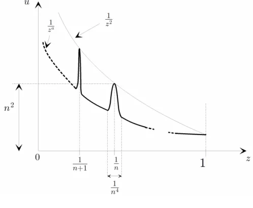
In general, one uses for r (z) the following function r (z) = ϕa(z) with 0 < a < 1. In the following example,
one has forced to change the form for r (z) in order to show the finite time stability. Let the function u be defined on ]0, 1] by its graph given in figure 1 and such that u¡1
n¢ = n
2 for n ≥ 1 and 0 < a < 1.
Figure 1. graph of u(z)
Let r(z) = ½ 0 if z = 0 1 u(z) if z 6= 0
then r is a continuous positive definite function and Z 1 0 dz r(z) = Z 1 0 u(z) dz ≤ Z 1 0 dz za + ∞ X n=2 1 n2 <+∞.
Consider the continuous function
f(x) = ½0 if x = 0 r(x2 ) 2x if x 6= 0 As fµ 1 n ¶ ≤ 2 −1 nu ¡ 1 n2 ¢ ≤ 1 2n3,
f is continuous at the origin and thus onR. Consider the system ˙x = f (x) , x∈R.
V (x) = x2 is a Lyapunov function for the system and ˙
V (x) ≤ −r (V (x)) .
So, the system is finite time stable. Nevertheless, there is no function ϕb with 0 < b < 1 such that r is
bounded below by ϕb.
6 Conclusion
A necessary and a sufficient condition for finite time stability of non autonomous continuous systems are given. As mentioned, there is still a gap to obtain necessary and sufficient conditions. The main difficulty comes from the non existence of the flow for only continuous systems and the non continuity of the settling time. Thus it is not an easy task to prove the existence of a Lyapunov function satisfying condition 7 under the hypothesis of finite time stability of the origin. However, with the given sufficient conditions, it is possible to investigate the problem of finite time stabilization for general continuous and non autonomous systems.
Acknowledgment
The authors thank the referees for careful reading and helpful suggestions on the improvement of the manuscript.
References
S.P. Bhat and D.S. Bernstein, “Continuous Finite-Time Stabilization of the Translational and Rotational Double Integrator”, IEEE Trans. Automat. Control, 43(5), pp. 678–682, 1998.
S.P. Bhat and D.S. Bernstein, “Finite Time Stability of Continuous Autonomous Systems”, SIAM J. Control Optim., 38(3), pp. 751–766, 2000.
W. Hahn, Theory and Application of Liapunov’s Direct Method, n.J., Prentice-Hall inc., 1963. V.T. Haimo, “Finite Time Controllers”, SIAM J. Control Optim., 24(4), pp. 760–770, 1986.
J.K. Hale, Ordinary Differential Equations, 2nd Edition, Pure and applied mathematics XXI, Krieger, 1980.
Y. Hong, “Finite-Time Stabilization and Stabilizability of a Class of Controllable Systems”, Systems Control Lett., 46, pp. 231–236, 2002.
Y. Hong, J. Huang and Y. Xu, “On an Output Feedback Finite-Time Stabilization Problem”, IEEE Trans. Automat. Control, 46, pp. 305–309, 2001.
Y. Hong, Y. Xu and J. Huang, “Finite-Time Control for Robot Manipulators”, Systems Control Lett., 46, pp. 243–253, 2002.
H.K. Khalil, Nonlinear Systems, NJ 07458, Upper Saddle River: Prentice-Hall, 1996.
A.M. Lyapunov, “Stability of Motion: General Problem”, Internat. J. Control, 55(3), pp. 520–790, lyapunov Centenary issue, 1992.
E. Moulay and W. Perruquetti, “Finite Time Stability of Non Linear Systems”, in IEEE Conference on Decision and Control, Hawaii, USA, 2003, pp. 3641–3646.
E. Moulay and W. Perruquetti, “Finite Time Stability and Stabilization of a Class of Continuous Systems”, J. Math. Anal. Appl., 323(2), pp. 1430–1443, 2006a.
E. Moulay and W. Perruquetti, Finite-time stability and stabilization: state of the art, in Advances in Variable Structure and Sliding Mode Control, 334, Lecture Notes in Control and Information Sciences, Springer-Verlag, 2006b.
W. Perruquetti and S. Drakunov, “Finite Time Stability and Stabilisation”, in IEEE Conference on De-cision and Control, Sydney, Australia, 2000.
E. Ryan, “Singular Optimal Controls for Second-Order Saturating Systems”, Internat. J. Control, 3(4), pp. 549–564, 1979.